Sentence Meta-Embeddings for Unsupervised Semantic Textual Similarity

Sentence Meta-Embeddings for Unsupervised Semantic Textual Similarity

Nina Poerner∗†and Ulli Waltinger†and Hinrich Sch ¨utze∗ ∗

Center for Information and Language Processing, LMU Munich, Germany †_{Corporate Technology Machine Intelligence (MIC-DE), Siemens AG Munich, Germany}

poerner@cis.uni-muenchen.de | inquiries@cislmu.org

Abstract

We address the task of unsupervised Seman-tic Textual Similarity (STS) by ensembling di-verse pre-trained sentence encoders into sen-tence meta-embeddings. We apply, extend and evaluate different meta-embedding meth-ods from the word embedding literature at the sentence level, including dimensionality re-duction (Yin and Sch¨utze,2016), generalized Canonical Correlation Analysis (Rastogi et al., 2015) and cross-view auto-encoders ( Bolle-gala and Bao, 2018). Our sentence meta-embeddings set a new unsupervised State of The Art (SoTA) on the STS Benchmark and on the STS12–STS16 datasets, with gains of be-tween 3.7% and 6.4% Pearson’srover single-source systems.

1 Introduction

Word meta-embeddings have been shown to exceed single-source word embeddings on word-level se-mantic benchmarks (Yin and Sch¨utze,2016; Bolle-gala and Bao,2018). Presumably, this is because they combine the complementary strengths of their components.

There has been recent interest in pre-trained “uni-versal” sentence encoders, i.e., functions that en-code diverse semantic features of sentences into fixed-size vectors (Conneau et al., 2017). Since these sentence encoders differ in terms of their ar-chitecture and training data, we hypothesize that their strengths are also complementary and that they can benefit from meta-embeddings.

To test this hypothesis, we adapt different meta-embedding methods from the word meta-embedding lit-erature. These include dimensionality reduction (Yin and Sch¨utze,2016), cross-view autoencoders (Bollegala and Bao,2018) and Generalized Canon-ical Correlation Analysis (GCCA) (Rastogi et al.,

2015). The latter method was also used byPoerner

and Sch¨utze(2019) for domain-specific Duplicate Question Detection.

Our sentence encoder ensemble includes three models from the recent literature: Sentence-BERT (Reimers and Gurevych,2019), the Universal

Sen-tence Encoder (Cer et al., 2017) and averaged

ParaNMT vectors (Wieting and Gimpel, 2018).

Our meta-embeddings outperform every one of their constituent single-source embeddings on

STS12–16 (Agirre et al., 2016) and on the STS

Benchmark (Cer et al.,2017). Crucially, since our meta-embeddings are agnostic to the contents of their ensemble, future improvements may be possi-ble by adding new encoders.

2 Related work

2.1 Word meta-embeddings

Word embeddings are functions that map word types to vectors. They are typically trained on un-labeled corpora and capture word semantics (e.g.,

Mikolov et al.(2013);Pennington et al.(2014)). Word meta-embeddings combine ensembles of

word embeddings by various operations:Yin and

Sch¨utze(2016) use concatenation, SVD and

lin-ear projection,Coates and Bollegala(2018) show

that averaging word embeddings has properties

similar to concatenation. Rastogi et al. (2015)

apply generalized canonical correlation analysis

(GCCA) to an ensemble of word vectors.Bollegala

and Bao(2018) learn word meta-embeddings

us-ing autoencoder architectures.Neill and Bollegala

(2018) evaluate different loss functions for

autoen-coder word meta-embeddings, whileBollegala et al.

(2018) explore locally linear mappings.

2.2 Sentence embeddings

Sentence embeddings are methods that produce one vector per sentence. They can be grouped into two categories:

F1(e.g., SBERT) . . . FJ(e.g., USE) (pre-trained encoders) S⊂S(e.g., BWC) (unlabeled corpus) X1∈R |S|×d1 .. . XJ∈R|S|×dJ

(cached training data)

Fit meta-embedding params (e.g.,Θfor GCCA)

(see Sections3.2,3.3,3.4) Fmeta _(s 1, s2) (sentence pair) ˆ y= cos(Fmeta (s1),Fmeta(s2)) (predicted sentence similarity score)

Figure 1: Schematic depiction: Trainable sentence meta-embeddings for unsupervised STS.

(a) Word embedding average sentence encoders take a (potentially weighted) average of pre-trained word embeddings. Despite their inability to under-stand word order, they are surprisingly effective on sentence similarity tasks (Arora et al., 2017;

Wieting and Gimpel,2018;Ethayarajh,2018) (b) Complex contextualized sentence encoders, such as Long Short Term Memory Networks

(LSTM) (Hochreiter and Schmidhuber, 1997) or

Transformers (Vaswani et al.,2017). Contextual-ized encoders can be pre-trained as unsupervised language models (Peters et al.,2018;Devlin et al.,

2019), but they are usually improved on supervised transfer tasks such as Natural Language Inference (Bowman et al.,2015).

2.3 Sentence meta-embeddings

Sentence meta-embeddings have been explored less frequently than their word-level counterparts.Kiela et al.(2018) create meta-embeddings by training an LSTM sentence encoder on top of a set of dy-namically combined word embeddings. Since this approach requires labeled data, it is not applicable to unsupervised STS.

Tang and de Sa(2019) train a Recurrent Neural Network (RNN) and a word embedding average encoder jointly on a large corpus to predict similar representations for neighboring sentences. Their approach trains both encoders from scratch, i.e., it cannot be used to combine existing encoders.

Poerner and Sch¨utze(2019) propose a GCCA-based multi-view sentence encoder that combines domain-specific and generic sentence embeddings for unsupervised Duplicate Question Detection. In this paper, we extend their approach by exploring a wider range of meta-embedding methods and an ensemble that is more suited to STS.

2.4 Semantic Textual Similarity (STS)

Semantic Textual Similarity (STS) is the task of rating the similarity of two natural language sen-tences on a real-valued scale. Related applications

are semantic search, duplicate detection and sen-tence clustering.

Supervised SoTA systems for STS typically ap-ply cross-sentence attention (Devlin et al., 2019;

Raffel et al.,2019). This means that they do not scale well to many real-world tasks. Supervised

“siamese” models (Reimers and Gurevych,2019)

on the other hand, while not competitive with cross-sentence attention, can cache cross-sentence embeddings independently of one another. For instance, to calculate the pairwise similarities ofN sentences, a cross-sentence attention system must calculate

O(N2)slow sentence pair embeddings, while the

siamese model calculatesO(N)slow sentence

em-beddings andO(N2)fast vector similarities. Our meta-embeddings are also cacheable (and hence scalable), but they do not require supervi-sion.

3 Sentence meta-embedding methods

Below, we assume access to an ensemble of pre-trained sentence encoders, denotedF₁. . .F_J. Ev-eryFj maps from the (infinite) set of possible sen-tencesSto a fixed-sizedj-dimensional vector.

Word meta-embeddings are usually learned from a finite vocabulary of word types (Yin and Sch¨utze,

2016). Sentence embeddings lack such a

“vocabu-lary”, as they can encode any member ofS.

There-fore, we train on a sampleS⊂_S, i.e., on a corpus of unlabeled sentences.

3.1 Naive meta-embeddings

We create naive sentence meta-embeddings by con-catenating (Yin and Sch¨utze,2016) or averaging1 (Coates and Bollegala,2018) sentence embeddings.

Fconc(s0) =   ˆ F₁(s0) . . . ˆ F_J(s0)  

1_{If embeddings have different dimensionalities, we pad the} shorter ones with zeros.

Favg(s0) =X j

ˆ

F_j(s0)

J

Note that we length-normalize all embeddings to ensure equal weighting:

ˆ

F_j(s) = Fj(s)

||Fj(s)||2 3.2 SVD

Yin and Sch¨utze (2016) use Singular Value De-composition (SVD) to compactify concatenated

word embeddings. The method is

straightfor-ward to extend to sentence meta-embeddings. Let Xconc∈R|S|×

P

jdj _with

xconc_n =Fconc(sn)−_Es∈S[Fconc(s)]

LetUSVT ≈Xconcbe thed-truncated SVD. The

SVD meta-embedding of a new sentences0is:

Fsvd(s0) =VT(Fconc(s0)−Es∈S[Fconc(s)])

3.3 GCCA

Given random vectorsx1,x2, Canonical

Correla-tion Analysis (CCA) finds linear projecCorrela-tions such that θT₁x1 and θT2x2 are maximally correlated.

Generalized CCA (GCCA) extends CCA to three

or more random vectors.Bach and Jordan(2002)

show that a variant of GCCA reduces to a general-ized eigenvalue problem on block matrices:

ρ   Σ1,1 0 0 0 Σ... 0 0 0 ΣJ,J     θ1 . . . θJ   =   0 Σ... Σ1,J Σ... 0 Σ... ΣJ,1 Σ... 0     θ1 . . . θJ   where Σj,j0 =_Es∈S[(F_j(s)−µ_j)(F_j0(s)−µ_j0)T] µ_j =Es∈S[Fj(s)]

For stability, we add _dτ

j Pdj

n=1diag(Σj,j)n to diag(Σj,j), whereτ is a hyperparameter. We stack the eigenvectors of the top-deigenvalues into

ma-trices Θj ∈ Rd×dj and define the GCCA

meta-embedding of sentences0as:

Fgcca(s0) = J

X

j=1

Θj(Fj(s0)−µj)

Fgcca _{corresponds to MV-DASE inPoerner and}

Sch¨utze(2019).

loss function

MSE MAE KLD (1-COS)2

number hidden layers

0 83.0/84.2 84.2/85.1 83.0/84.2 82.4/83.5 1 82.7/83.9 83.8/84.6 85.1/85.5 83.3/83.4 2 82.5/82.8 81.3/82.1 83.3/83.4 82.3/82.3

τ = 10−2 τ= 10−1 τ= 100 τ= 101 τ = 102

84.2/84.1 84.8/84.7 85.5/85.7 85.5/86.1 84.9/85.9

Table 1: Hyperparameter search on STS Benchmark de-velopment set for AE (top) and GCCA (bottom). Pear-son’sr×100/ Spearman’sρ×100.

3.4 Autoencoders (AEs)

Autoencoder meta-embeddings are trained by gra-dient descent to minimize some cross-embedding

reconstruction loss. For example,Bollegala and

Bao(2018) train feed-forward networks (FFN) to

encode two sets of word embeddings into a shared space, and then reconstruct them such that mean squared error with the original embeddings is mini-mized.Neill and Bollegala(2018) evaluate differ-ent reconstruction loss functions: Mean Squared Error (MSE), Mean Absolute Error (MAE), KL-Divergence (KLD) or squared cosine distance (1-COS)2.

We extend their approach to sentence encoders as follows: Every sentence encoderF_jhas a

train-able encoderEj : Rdj _{→ R}d_{and a trainable}

de-coderDj :Rd→Rdj, wheredis a hyperparameter.

Our training objective is to reconstruct every em-beddingxj0 from everyE_j(xj). This results inJ2

loss terms, which are jointly optimized:

L(x1. . .xJ) = X j X j0 l(xj0,D_j0(Ej(xj)))

wherelis one of the reconstruction loss functions listed above. The autoencoder meta-embedding of a new sentences0 is:

Fae(s0) =X j

Ej(Fj(s0))

4 Experiments 4.1 Data

We train on all sentences of length < 60 from

the first file (news.en-00001-of-00100) of the tok-enized, lowercased Billion Word Corpus (BWC) (Chelba et al.,2014) (∼302K sentences). We evalu-ate on STS12 – STS16 (Agirre et al.,2016) and the

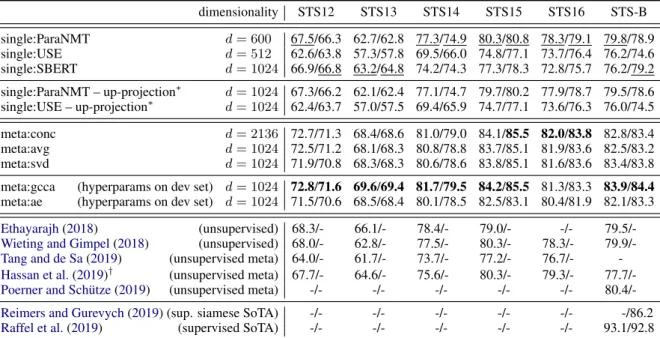
dimensionality STS12 STS13 STS14 STS15 STS16 STS-B single:ParaNMT d= 600 67.5/66.3 62.7/62.8 77.3/74.9 80.3/80.8 78.3/79.1 79.8/78.9 single:USE d= 512 62.6/63.8 57.3/57.8 69.5/66.0 74.8/77.1 73.7/76.4 76.2/74.6 single:SBERT d= 1024 66.9/66.8 63.2/64.8 74.2/74.3 77.3/78.3 72.8/75.7 76.2/79.2 single:ParaNMT – up-projection∗ d= 1024 67.3/66.2 62.1/62.4 77.1/74.7 79.7/80.2 77.9/78.7 79.5/78.6 single:USE – up-projection∗ d= 1024 62.4/63.7 57.0/57.5 69.4/65.9 74.7/77.1 73.6/76.3 76.0/74.5 meta:conc d= 2136 72.7/71.3 68.4/68.6 81.0/79.0 84.1/85.5 82.0/83.8 82.8/83.4 meta:avg d= 1024 72.5/71.2 68.1/68.3 80.8/78.8 83.7/85.1 81.9/83.6 82.5/83.2 meta:svd d= 1024 71.9/70.8 68.3/68.3 80.6/78.6 83.8/85.1 81.6/83.6 83.4/83.8

meta:gcca (hyperparams on dev set) d= 1024 72.8/71.6 69.6/69.4 81.7/79.5 84.2/85.5 81.3/83.3 83.9/84.4 meta:ae (hyperparams on dev set) d= 1024 71.5/70.6 68.5/68.4 80.1/78.5 82.5/83.1 80.4/81.9 82.1/83.3 Ethayarajh(2018) (unsupervised) 68.3/- 66.1/- 78.4/- 79.0/- -/- 79.5/-Wieting and Gimpel(2018) (unsupervised) 68.0/- 62.8/- 77.5/- 80.3/- 78.3/- 79.9/-Tang and de Sa(2019) (unsupervised meta) 64.0/- 61.7/- 73.7/- 77.2/- 76.7/- -Hassan et al.(2019)† (unsupervised meta) 67.7/- 64.6/- 75.6/- 80.3/- 79.3/- 77.7/-Poerner and Sch¨utze(2019) (unsupervised meta) -/- -/- -/- -/- -/- 80.4/-Reimers and Gurevych(2019) (sup. siamese SoTA) -/- -/- -/- -/- -/- -/86.2 Raffel et al.(2019) (supervised SoTA) -/- -/- -/- -/- -/- 93.1/92.8

Table 2: Results on STS12–16 and STS Benchmark test set. STS12–16: mean Pearson’sr×100/ Spearman’s ρ×100. STS Benchmark: overall Pearson’sr×100 / Spearman’sρ×100. Evaluated by SentEval (Conneau and Kiela,2018).Boldface:best in column (except supervised). Underlined: best single-source method.∗Results for up-projections are averaged over 10 random seeds. †Unweighted average computed fromHassan et al.(2019, Table 8). There is no supervised SoTA on STS12–16, as they are unsupervised benchmarks.

2017).2 These datasets consist of triples(s1, s2, y),

where s1, s2 are sentences andy is their ground

truth semantic similarity. The task is to predict similarity scoresyˆthat correlate well withy. We predictyˆ= cos(F(s1),F(s2)).

4.2 Metrics

Previous work on STS differs with respect to (a) the correlation metric and (b) how to aggregate the sub-testsets of STS12–16. To maximize comparability,

we report both Pearson’srand Spearman’sρ. On

STS12–16, we aggregate by a non-weighted aver-age, which diverges from the original shared tasks (Agirre et al.,2016) but ensures comparability with more recent baselines (Wieting and Gimpel,2018;

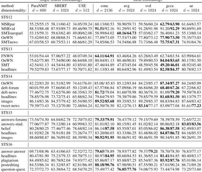
Ethayarajh,2018). Results for individual STS12– 16 sub-testsets can be found in the Appendix.

4.3 Ensemble

We select our ensemble according to the following criteria: Every encoder should have near-SoTA per-formance on the unsupervised STS benchmark, and the encoders should not be too similar with regards to their training regime. For instance, we do not

2

We use SentEval for evaluation (Conneau and Kiela, 2018). Since original SentEval does not support the unsu-pervised STS Benchmark, we use a non-standard repository (https://github.com/sidak/SentEval). We man-ually add the missing STS13-SMT subtask.

useEthayarajh(2018), which is a near-SoTA unsu-pervised method that uses the same word vectors as ParaNMT (see below).

We choose the Universal Sentence Encoder

(USE)3 (Cer et al., 2018), which is a

Trans-former trained on skip-thought, conversation re-sponse prediction and Natural Language Inference

(NLI), Sentence-BERT (SBERT)4 (Reimers and

Gurevych, 2019), which is a pre-trained BERT

transformer finetuned on NLI, and ParaNMT5(

Wi-eting and Gimpel,2018), which averages word and 3-gram vectors trained on backtranslated similar sentence pairs. To our knowledge, ParaNMT is the current single-source SoTA on the unsupervised STS Benchmark.

4.4 Hyperparameters

We set d = 1024in all experiments, which

cor-responds to the size of the biggest single-source

embedding (SBERT). The value ofτ (GCCA), as

well as the autoencoder depth and loss function are tuned on the STS Benchmark development set (see

3

https://tfhub.dev/google/ universal-sentence-encoder/2 4_{https://github.com/UKPLab/}

sentence-transformers. We use the large-nli-mean-tokensmodel, which wasnotfinetuned on STS.

5_{https://github.com/jwieting/} para-nmt-50m

full without without without

ensemble ParaNMT USE SBERT

meta:svd 85.0/85.4 79.6/81.3 79.7/81.4 83.7/83.5 meta:gcca 85.5/86.1 84.9/84.8 83.8/83.8 85.4/85.4 meta:ae 85.1/85.5 76.5/80.3 82.5/83.5 28.7/41.0

Table 3: Ablation study: Pearson’s r×100 / Spear-man’s ρ×100 on STS Benchmark development set when one encoder is left out.

Table1). We train the autoencoder for a fixed num-ber of 500 epochs with a batch size of 10,000. We

use the Adam optimizer (Kingma and Ba, 2014)

withβ1 = 0.9,β2 = 0.999and learning rate0.001. 4.5 Baselines

Our main baselines are our single-source

embed-dings. Wieting and Kiela(2019) warn that

high-dimensional sentence representations can have an advantage over low-dimensional ones, i.e., our meta-embeddings might be better than lower-dimensional single-source embeddings due to size alone. To exclude this possibility, we also

up-project smaller embeddings by a randomd×dj

matrix sampled from:

U(−_p1

dj

,p1 dj

)

Since the up-projected sentence embeddings per-form slightly worse than their originals (see Table

2, rows 4–5), we are confident that performance

gains by our meta-embeddings are due to content rather than size.

4.6 Results

Table 2 shows that even the worst of our

meta-embeddings consistently outperform their single-source components. This underlines the overall usefulness of ensembling sentence encoders, irre-spective of the method used.

GCCA outperforms the other meta-embeddings on five out of six datasets. We set a new unsu-pervised SoTA on the unsuunsu-pervised STS Bench-mark test set, reducing the gap with the supervised

siamese SoTA of Reimers and Gurevych (2019)

from 7% to 2% Spearman’sρ.

Interestingly, the naive meta-embedding meth-ods (concatenation and averaging) are competitive with SVD and the autoencoder, despite not needing any unsupervised training. In the case of concatena-tion, this comes at the cost of increased dimension-ality, which may be problematic for downstream

ap-plications. The naive averaging method byCoates

and Bollegala(2018) however does not have this problem, while performing only marginally worse than concatenation.

4.7 Ablation

Table3 shows that all single-source embeddings

contribute positively to the meta-embeddings, which supports their hypothesized complementar-ity. This result also suggests that further improve-ments may be possible by extending the ensemble.

4.8 Computational cost 4.8.1 Training

All of our meta-embeddings are fast to train, either because they have closed-form solutions (GCCA and SVD) or because they are lightweight feed-forward nets (autoencoder). The underlying sen-tence encoders are more complex and slow, but since we do not update them, we can apply them to the unlabeled training data once and then reuse the results as needed.

4.8.2 Inference

As noted in Section2.4, cross-sentence attention

systems do not scale well to many real-world STS-type tasks, as they do not allow individual

sen-tence embeddings to be cached. Like Reimers

and Gurevych (2019), our meta-embeddings do not have this problem. This should make them more suitable for tasks like sentence clustering or real-time semantic search.

5 Conclusion

Inspired by the success of word meta-embeddings, we have shown how to apply different meta-embedding techniques to ensembles of sentence en-coders. All sentence meta-embeddings consistently outperform their individual single-source compo-nents on the STS Benchmark and the STS12–16 datasets, with a new unsupervised SoTA set by our GCCA embeddings. Because sentence meta-embeddings are agnostic to the size and specifics of their ensemble, it should be possible to add new encoders to the ensemble, potentially improving performance further.

Acknowledgments. This work was supported by Siemens AG and by the European Research Coun-cil (# 740516).

References

Eneko Agirre, Carmen Banea, Daniel Cer, Mona Diab, Aitor Gonzalez-Agirre, Rada Mihalcea, German Rigau, and Janyce Wiebe. 2016. SemEval-2016 Task 1: Semantic textual similarity, monolingual and cross-lingual evaluation. InInternational Workshop on Semantic Evaluation, pages 497–511, San Diego, USA.

Sanjeev Arora, Yingyu Liang, and Tengyu Ma. 2017. A simple but tough-to-beat baseline for sentence em-beddings. InICLR, Toulon, France.

Francis R Bach and Michael I Jordan. 2002. Kernel independent component analysis. JMLR, 3:1–48. Danushka Bollegala and Cong Bao. 2018. Learning

word meta-embeddings by autoencoding. In COL-ING, pages 1650–1661, Santa Fe, USA.

Danushka Bollegala, Kohei Hayashi, and Ken-ichi Kawarabayashi. 2018. Think globally, embed lo-cally – lolo-cally linear meta-embedding of words. In ICJAI, pages 3970–3976, Stockholm, Sweden. Samuel R Bowman, Gabor Angeli, Christopher Potts,

and Christopher D Manning. 2015. A large anno-tated corpus for learning natural language inference. InEMNLP, pages 632–642, Lisbon, Portugal. Daniel Cer, Mona Diab, Eneko Agirre, Inigo

Lopez-Gazpio, and Lucia Specia. 2017. SemEval-2017 task 1: Semantic textual similarity multilingual and crosslingual focused evaluation. In International Workshop on Semantic Evaluation, pages 1–14, Van-couver, Canada.

Daniel Cer, Yinfei Yang, Sheng-yi Kong, Nan Hua, Nicole Limtiaco, Rhomni St John, Noah Constant, Mario Guajardo-Cespedes, Steve Yuan, Chris Tar, et al. 2018. Universal Sentence Encoder for English. InEMNLP, pages 169–174, Brussels, Belgium. Ciprian Chelba, Tomas Mikolov, Mike Schuster, Qi Ge,

Thorsten Brants, Phillipp Koehn, and Tony Robin-son. 2014. One billion word benchmark for mea-suring progress in statistical language modeling. In INTERSPEECH, pages 2635–2639, Singapore. Joshua Coates and Danushka Bollegala. 2018.

Frus-tratingly easy embedding – computing meta-embeddings by averaging source word meta-embeddings. In NAACL-HLT, pages 194–198, New Orleans, USA.

Alexis Conneau and Douwe Kiela. 2018.SentEval: An evaluation toolkit for universal sentence representa-tions. InLREC, pages 1699–1704, Miyazaki, Japan. Alexis Conneau, Douwe Kiela, Holger Schwenk, Lo¨ıc Barrault, and Antoine Bordes. 2017. Supervised learning of universal sentence representations from natural language inference data. InEMNLP, pages 670–680, Copenhagen, Denmark.

Jacob Devlin, Ming-Wei Chang, Kenton Lee, and Kristina Toutanova. 2019. BERT: Pre-training of deep bidirectional transformers for language under-standing. InNAACL, New Orleans, USA.

Kawin Ethayarajh. 2018. Unsupervised random walk sentence embeddings: A strong but simple baseline. In Workshop on Representation Learning for NLP, pages 91–100, Melbourne, Australia.

Basma Hassan, Samir E Abdelrahman, Reem Bahgat, and Ibrahim Farag. 2019. UESTS: An unsupervised ensemble semantic textual similarity method. IEEE Access, 7:85462–85482.

Sepp Hochreiter and J¨urgen Schmidhuber. 1997. Long short-term memory. Neural computation, 9(8):1735–1780.

Douwe Kiela, Changhan Wang, and Kyunghyun Cho. 2018.Dynamic meta-embeddings for improved sen-tence representations. InEMNLP, pages 1466–1477, Brussels, Belgium.

Diederik P Kingma and Jimmy Ba. 2014. Adam: A method for stochastic optimization. arXiv preprint arXiv:1412.6980.

Tomas Mikolov, Ilya Sutskever, Kai Chen, Greg S Cor-rado, and Jeff Dean. 2013. Distributed representa-tions of words and phrases and their composition-ality. InNeurIPS, pages 3111–3119, Lake Tahoe, USA.

James O’ Neill and Danushka Bollegala. 2018. Angular-based word meta-embedding learning. arXiv preprint arXiv:1808.04334.

Jeffrey Pennington, Richard Socher, and Christopher Manning. 2014. GloVe: Global vectors for word representation. InEMNLP, pages 1532–1543, Doha, Qatar.

Matthew Peters, Mark Neumann, Mohit Iyyer, Matt Gardner, Christopher Clark, Kenton Lee, and Luke Zettlemoyer. 2018. Deep contextualized word repre-sentations. InNAACL-HLT, pages 2227–2237, New Orleans, USA.

Nina Poerner and Hinrich Sch¨utze. 2019. Multi-view domain adapted sentence embeddings for low-resource unsupervised duplicate question detection. InEMNLP-IJCNLP, Hong Kong, China.

Colin Raffel, Noam Shazeer, Adam Roberts, Katherine Lee, Sharan Narang, Michael Matena, Yanqi Zhou, Wei Li, and Peter J Liu. 2019. Exploring the limits of transfer learning with a unified text-to-text trans-former.arXiv preprint arXiv:1910.10683.

Pushpendre Rastogi, Benjamin Van Durme, and Raman Arora. 2015. Multiview LSA: Representation learn-ing via generalized CCA. In NAACL-HLT, pages 556–566, Denver, USA.

Nils Reimers and Iryna Gurevych. 2019. Sentence-bert: Sentence embeddings using siamese bert-networks. InEMNLP-IJCNLP, Hong Kong, China. Shuai Tang and Virginia R de Sa. 2019. Improving

sen-tence representations with multi-view frameworks. InInterpretability and Robustness for Audio, Speech and Language Workshop, Montreal, Canada. Ashish Vaswani, Noam Shazeer, Niki Parmar, Jakob

Uszkoreit, Llion Jones, Aidan N Gomez, Łukasz Kaiser, and Illia Polosukhin. 2017. Attention is all you need. InNeurIPS, pages 5998–6008, Long Beach, USA.

John Wieting and Kevin Gimpel. 2018. ParaNMT-50M: Pushing the limits of paraphrastic sentence em-beddings with millions of machine translations. In ACL, pages 451–462, Melbourne, Australia. John Wieting and Douwe Kiela. 2019. No training

required: Exploring random encoders for sentence classification. InICLR, New Orleans, USA. Wenpeng Yin and Hinrich Sch¨utze. 2016. Learning

word meta-embeddings. InACL, pages 1351–1360, Berlin, Germany.

single-source embeddings meta-embeddings

method: ParaNMT SBERT USE conc avg svd gcca ae

dimensionality: d= 600 d= 1024 d= 512 d= 2136 d= 1024 d= 1024 d= 1024 d= 1024 STS12 MSRpar 55.25/55.15 58.11/60.42 34.05/39.24 60.13/60.53 58.90/59.71 59.56/60.24 62.79/63.90 61.64/63.57 MSRvid 88.53/88.48 87.93/89.73 89.46/90.75 91.51/92.16 91.29/91.92 91.28/91.98 91.20/92.29 90.69/91.69 SMTeuroparl 53.15/59.31 59.63/62.40 49.00/62.08 58.99/64.02 60.16/64.73 57.03/62.17 56.40/61.23 55.13/60.14 OnWN 73.42/69.82 68.08/68.51 71.66/65.81 77.89/73.05 77.53/73.00 77.80/73.12 77.90/73.50 75.35/73.03 SMTnews 67.03/58.53 60.75/53.11 68.66/61.29 74.85/66.53 74.54/66.88 73.73/66.48 75.75/67.31 74.91/64.76 STS13 FNWN 53.01/54.44 57.06/57.22 48.07/49.34 64.11/64.91 63.46/64.26 63.28/63.49 62.74/63.54 63.99/64.61 OnWN 75.62/75.80 77.54/80.00 66.64/68.10 80.84/81.13 80.46/80.81 79.89/80.53 84.04/83.65 80.17/81.50 SMT 42.54/41.13 44.54/44.80 43.85/41.80 47.46/44.89 47.87/45.04 48.59/45.58 49.20/46.01 48.92/45.40 headlines 79.52/79.83 73.67/77.17 70.70/71.82 81.13/83.48 80.64/82.96 81.49/83.54 82.58/84.37 80.78/82.13 STS14 OnWN 82.22/83.20 81.51/82.99 74.61/76.01 85.08/ 85.83 85.12/85.84 84.23/85.17 87.34/87.27 84.24/85.09 deft-forum 60.01/59.49 57.66/60.45 50.12/49.43 67.57/66.84 67.09/66.19 66.84/66.20 68.40/67.26 67.22/66.82 deft-news 77.46/72.75 72.62/76.80 68.35/63.35 81.72/79.04 81.60/78.98 80.36/78.31 81.09/79.20 79.59/78.83 headlines 78.85/76.98 73.72/75.41 65.88/62.34 79.64/79.93 79.39/79.86 79.85/79.59 81.68/81.50 80.13/79.77 images 86.14/83.36 84.57/79.42 85.54/80.55 89.52/85.68 89.35/85.51 89.29/85.37 88.83/84.83 87.64/83.42 tweet-news 79.39/73.43 75.12/70.80 72.48/64.24 82.50/76.50 82.12/76.13 83.14/77.17 83.09/77.04 81.61/77.23 STS15 answers-forums 73.54/74.50 64.04/62.78 72.70/75.02 79.33/79.91 78.47/79.12 79.15/79.69 78.39/78.59 72.65/72.21 answers-stud. 77.06/77.87 79.12/80.14 60.99/63.32 81.01/82.10 80.15/81.45 81.02/82.14 80.86/82.18 83.03/83.56 belief 80.28/80.25 77.46/77.46 78.68/82.14 86.14/87.58 85.55/87.01 85.05/86.02 86.38/87.58 82.49/83.07 headlines 81.92/82.28 78.91/81.88 73.26/74.77 83.20/86.03 83.33/86.25 83.48/86.02 84.87/86.72 84.16/85.53 images 88.60/88.87 86.76/89.02 88.39/90.34 90.92/91.95 90.86/91.92 90.46/91.59 90.34/91.85 90.26/91.35 STS16 answer-answer 69.71/68.96 63.41/66.63 72.52/72.72 79.65/78.89 78.93/77.82 79.37/79.21 78.70/78.50 76.83/77.17 headlines 80.47/81.90 75.23/79.33 69.70/75.11 80.97/84.95 80.60/84.53 81.36/85.14 81.41/84.85 80.40/83.17 plagiarism 84.49/85.62 80.78/82.04 74.93/77.42 85.86/87.17 85.88/87.25 85.54/87.36 85.92/87.76 85.01/86.14 postediting 84.53/86.34 81.32/85.87 82.81/86.49 88.18/90.76 87.98/90.51 87.55/90.21 87.01/90.24 86.71/89.28 question-quest. 72.37/72.73 63.38/64.72 68.54/70.25 75.49/77.42 76.05/77.76 74.08/75.93 73.44/74.98 73.25/73.60

Table 4: Pearson’sr/ Spearman’sρ×100on individual sub-testsets of STS12–STS16.Boldface: best method in row.