Selected Problems for High-Dimensional Data - Quantile and Errors-in-Variables Regressions.

Data – Quantile and Errors-in-Variables

Regressions

by

Seyoung Park

A dissertation submitted in partial fulfillment

of the requirements for the degree of

Doctor of Philosophy

(Statistics)

in The University of Michigan

2016

Doctoral Committee:

Professor Xuming He, Co-Chair

Assistant Professor Shuheng Zhou, Co-Chair Professor Timothy D. Johnson

I would like to express my deepest gratitude to my advisors Xuming He, Shuheng Zhou and Kerby Shedden whose continuous guidance and support has been the greatest source of encouragement throughout my PhD. I feel very lucky to have them as my advisors, and their warm encouragement and support make me have such a wonderful experience as a PhD student.

I would like to thank my committee member, Professor Timothy Johnson for his valuable time and suggestions on my thesis research.

I also thank Professor Alexandre Belloni and Professor Po-Ling Loh for sharing codes with me.

The research in the thesis is supported by NSF Grants 13-07566, DMS-13-16731, and the Elizabeth Caroline Crosby Research Award from the Advance Program at the University of Michigan.

Last, but not the least, I would like to thank my parents and sister for their unconditional love and endless support.

ACKNOWLEDGEMENTS . . . ii

LIST OF FIGURES . . . v

LIST OF TABLES . . . x

CHAPTER 1.

Introduction

1.1 Multiple Quantile Regression with High Dimensional Covariates 1 1.2 Matrix Variate Model . . . 3

2.

Multiple Quantile Regression with High

Dimensional Covariates

2.1 Introduction . . . 6

2.2 Model and Method . . . 7

2.3 Theoretical Properties . . . 10

2.4 Implementation . . . 15

2.5 Theoretical Properties (continued) . . . 17

2.6 Post–Selection Joint Quantile Regression . . . 19

2.7 Numerical Studies . . . 22 2.8 Application . . . 27 2.9 Conclusion . . . 30 2.10 Supplementary Material . . . 31 3.

Errors-in-Variables Regression

3.3 The Lasso-type and Conic Programming Estimators . . . 59

3.4 Simulations . . . 60

3.5 Optimization Error . . . 68

4.1 Introduction . . . 70

4.2 Nodewise Regression Procedure . . . 73

4.3 Projected Graphical Lasso Method . . . 75

4.4 Simulations . . . 76

4.5 Analysis of Hawkmoth Neural Encoding Data . . . 80

4.5.1 Fit of the Additive Covariance Model . . . 82

4.5.2 Estimating the Trace Parameter . . . 87

4.5.3 Graphical Structures . . . 91

4.5.4 Mean-Variance Analysis . . . 95

4.5.5 Regression Analysis . . . 97

5.

Future Work

5.1 Hypothesis Testing for Multiple Quantiles . . . 103

5.2 Theory and Methods for EIV Regression . . . 104

Bibliography . . . 105

Figure

2.1 Results for Example 2.7.1 (top), 2.7.2 (middle) and 2.7.3 (below): Include false positives(left), false negatives (middle) and the stability measures (right). Four competing procedures are evaluated: Lasso, ALasso, FAL and Dantzig. . . 26 2.2 Results for Example 2.7.4 (top) and 2.7.5 (below): Include false

positives (left), false negatives (middle) and the stability measures (right). Four competing procedures are evaluated: Lasso, ALasso, FAL and Dantzig. . . 27 3.1 Plots for the Lasso estimator with a constraint kβk1 ≤ Rkβ∗k1,

where β∗ = [0.5,· · · ,0.5,0,· · · ,0]T_{, where d = 10 0.6n/log(m).}

Step size η = 2kAk2 are chosen. Five values are used for R and λ change from 0 to 0.5, when m = 400 and n = 100. A is generated using AR(1) model with parameterρA= 0.5, andB = 0.1B∗, where

B∗ follows AR(1) model with parameter 0.8. The standard deviation of noise is σ= 1. The Signal-to-noise ratio S/M is 1.35. . . 63 3.2 Plots for the Lasso estimator under the same settings used in Figure

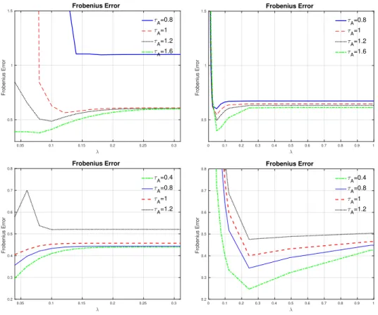
3.1 except thatB = 0.7B∗. The Signal-to-noise ratio S/M is 0.50. . 64 3.3 Plots for the Lasso estimator with a constraint kβk1 ≤ Rkβ∗k1,

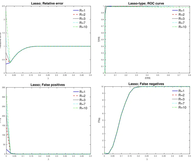
where β∗ = [0.9,· · · ,0.9,0,· · · ,0]T, where d = 20 1.2n/log(m). Step sizeη= 2kAk2 are chosen. The other settings are exactly same as the one used in Figure 3.2. The Signal-to-noise ratio S/M is 0.60. 65 3.4 Plots for the Lasso estimator. The top plots are when m = 400,

n= 100 andβ∗ = [0.5,· · · ,0.5,0,· · · ,0]T_{, where d= 10. The below}

plots are when m= 600, n = 200 and β∗ = [0.9,· · · ,0.9,0,· · · ,0]T_,

where d = 20. A is generated using AR(1) model with parameter

ρA = 0.5, and B follows random model. The standard deviation of

noise is σ= 1. The Signal-to-noise ratio S/M for top and below are 0.50 and 0.65, respectively. . . 66

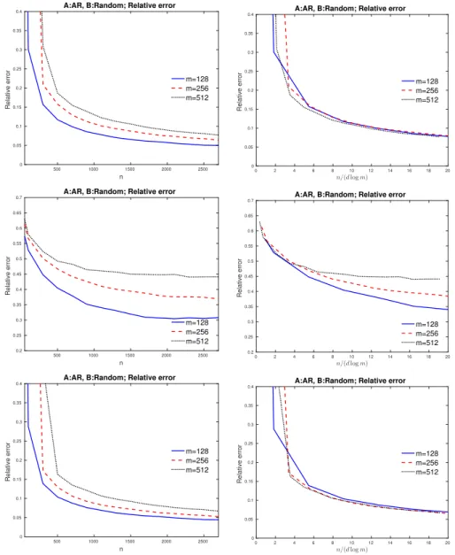
The below plot is for Conic withd= [m1/3]. The left plot is an error plot with m ∈ {128,256,512} and n changes from 50 to 2700. A is generated using AR(1) model with parameter ρA = 0.5, and B

follows random model. The standard deviation of noise is σ= 0.5. . 67 3.6 Plot for the optimization error log(kβt − βbk2) and statistical

er-ror log(kβt _−β∗_k

2) for each tth iterate. The blue lines and the red lines correspond to the statistical error and the optimization error, respectively. Each plot shows the solution path using 20 different starting points. We fix m = 500, n = 200 and β∗ = [1,0.9,· · · ,0.1,0,· · ·,0]T_{, where the first 10 components are}

non-zero. A and B are generated using AR(1) model with parameter

ρA= 1 and the random graph model, respectively. . . 69

4.1 The relative Frobenius error of the estimates Ab = Θb−1 (top) and b

B = Ωb−1 (below) when m = 400, n = 100 and the covariance

matrix Ais AR(1). The left figure and the right figure show the rel-ative Frobenius error of nodewise regression estimate and projected GLasso estimate, respectively. . . 78 4.2 The ROC curve of the estimates Θ whenb m = 400, n = 100. The

left figures and the right figures are when τ(A) = 1.5. . . 78 4.3 The recall and precision curves of the nodewise regression estimate

of Θ (top) and Ω (below), respectively, when m= 400,n = 100 and the covariance matrix A is AR(1). . . 79 4.4 The L2 error for the nodewise regression estimateAbwhen A is AR(1)

andB = 0.1B∗(left) orB = 0.5B∗, whereB∗ follows Random graph. The error versus the rescaled sample sizen/(d2logm) are plotted for three different m cases. . . 79 4.5 The performance results of the estimatesAbwhenτ(A) increases from

0.1 to 1.9; the dimensions are fixed at m = 200 and n = 200; the two plots show the L2 error and Frobenius error, respectively. . . 80

necker sum or product whenAis Star-Block (left) and AR(1) (right), respectively. The blue vertical line is the expected value of the statis-tic for the Kronecker product model. For the Star-Block model, the (mean, standard deviation) from the sum and product model are (0.0016,0.055) and (0.1184,0.2629), respectively. For the AR(1)

model, the sum and product model have (−0.0005,0.0223) and (0.0206,0.0671), respectively. . . 84 4.7 Histogram of the statistic S_off∗ for 500 bootstrap samples generated

from Kronecker sum and product estimates. The left and right figures are when the observed data X follows Kronecker sum and product models, respectively. The black vertical line indicates one observed value of Soff from a Kronecker sum (left) product model (right). . . 85 4.8 The histogram ofS_off∗ calculated from 200 generated random samples

using estimates of A and B from the Kronecker sum and product models. The blue bar indicates the observed statistic from the moth torque data X, and right bars and blue bars are from sum and product based samples. The two histograms are from moth J and moth L, respectively. . . 87 4.9 Normalized error paths for 50 samples (left) and the histogram of

tr(A)/m (right) for 200 samples when τA = 0.4 (top), τA = 1

(mid-dle) and τA = 1.8 (below). The dimension (m, n) = (400,100). For

the top plots, we use A = 0.4A∗, where A∗ follows AR(1) model, and B = 1.6B∗, where B∗ follows random model. For the middle and below plots, we use A =A∗ and B = B∗, and A = 1.8A∗ and

B = 0.2B∗, respectively. . . 89 4.10 Average of normalized error paths for 200 samples when A and B

are diagonal matrices. The left and right plots are when τA = 1 and

τA= 1.5, respectively. . . 90

4.11 Moth J and L(spike): Frobenius distance of the Kronekcer sum co-variance estimate obtained by using τ_bA = d, relative to rank-one

sample covariance matrix. . . 90 4.12 The graphical structure ofΘ from Kronecker sum model using node-b

wise regression method . . . 91

The left and the right plots correspond to moth J and L, respectively. 92 4.14 The diagonal components and the off-diagonal components ofΘ fromb

Kronecker sum model. Here off(k) records the off-diagonal compo-nents having the form (Θ)b _i,i−k fori= 1,· · · ,500. . . 93

4.15 The estimated graphical structure of Ω from Kronecker sum model. The left and the right plots for Moth J and L, respectively. . . 94 4.16 Torque ensembles for three clusters of Moth J. The average of

pair-wise correlations within the cluster 1, cluster 2 and cluster 3 are 0.6876, 0.7120, and 0.7322, respectively. The average of pairwise correlations between clusters 1&2, 1&3, and 2&3 are 0.3572, 0.1144, and 0.2125, respectively. The average and standard deviation of the torque mean within clusters are (0.3288, 0.2481), (0.1318, 0.2394) and (-0.3678, 0.2680), respectively. . . 94 4.17 The left plot shows three wingstroke paths for moth J. For the

wingstrokes w498 and w379, the correlation obtained from the data and the correlation calculated from Bb are 0.972 and 0.82,

respec-tively. Those values for the wingstrokesw498 andw432 are−0.47 and −0.35, respectively. The right plot includes the three wingstrokes paths for moth L. For the wingstrokesw289 and w272, the correlation from the data and the correlation calculated from Bb are 0.946 and

0.85, respectively. The values for the wingstrokes w289 and w99 are −0.79 and−0.71, respectively. . . 95 4.18 Scatter plots for the mean torque differences of wingstrokes and the

corresponding entries inBb (top) and Ω (below). . . .b 96

4.19 Histogram of R-squared estimates when β = 0 and X follows Kro-necker sum covariance model, where the estimated covariance ma-trices for moth M (phase) and moth M (spike) are used for left and right plots, respectively. . . 99 4.20 The estimated regression coefficients from the regular regression (ridge

regression and Scaled Lasso) and the errors-in-variables regression (EIV) for phase data set. . . 100

regression and Scaled Lasso) and the errors-in-variables regression (EIV) for spike data set. . . 101 4.22 The estimated regression coefficients from the regular regression (ridge

regression and Scaled Lasso) and the errors-in-variables regression (EIV) for phase data set. . . 101 4.23 The estimated regression coefficients from the regular regression (ridge

regression and Scaled Lasso) and the errors-in-variables regression (EIV) for spike data set. . . 102

Table

2.1

Notations used in the Chapter

2.2

Performance results of whole dataset

2.3

Performance results of 100 random partitions of the data

Metrics

4.1

The Notations

4.2

The simulated statistic

S

4.3

Explanatory power (R-squared)

Introduction

1.1

Multiple Quantile Regression with High Dimensional

Covariates

Quantile regression has become a widely used method to evaluate the effect of regressors on the conditional distribution of a response variable (Koenker, 2005). Compared to linear regression analysis, quantile regression is less sensitive to the mis-specification of error distributions and provides more comprehensive information on the relationship between the response variable and the covariates. It is important to study quantile regression in the high-dimensional setting because high-dimensional data arise from many modern application areas such as signal processing and ge-nomics. We focus on the cases where, p, the number of covariates, is greater than n, the sample size.

There has been a line of recent work on variable selection for quantile regression models (Li and Zhu, 2008; Zou and Yuan, 2008a,b; Wu and Liu, 2009). In the high-dimensional setting, the penalization methods with the`1 penalty (Belloni and Chernozhukov, 2011; Wang, 2013), weighted`1penalty (Zheng et al., 2013; Fan et al., 2014a) and smoothly clipped absolute deviation (SCAD) penalty (Wang et al., 2012;

Fan et al., 2014b) have been used to obtain consistent model selection. Belloni and Chernozhukov (2011) establish consistency in parameter estimation with the `1 penalty. Wang et al. (2012) consider the SCAD penalty, and show that the oracle estimate is one of the local minima of their non-convex optimization problem. Fan et al. (2014a) use the weighted`1 penalty based on the SCAD penalty function, and establish the model selection consistency and asymptotic normality.

Although the aforementioned work establish nice theoretical properties, empirical evidence shows that the sets of variables selected at two nearby quantiles are often unpleasantly different. The stability of selected variables across quantiles is desirable both for the purpose of interpreting results and for understanding the impact of a particular covariate on the conditional quantile functions. For example, a covariate that is selected at quantiles 0.5 and 0.6 but not at 0.55 would not be much appreciated unless there is a strong reason. The motivation and the main contribution of our work is to show joint modeling across quantiles could lead to stable models. Zou and Yuan (2008a,b), Bang and Jhun (2012), Jiang et al. (2013), Peng et al. (2014), and Volgushev et al. (2014) consider joint quantile regression and provide consistent estimators. He (1997), Dette and Volgushev (2008), Bondell et al. (2010), and Jang and Wang (2015) study non-crossing quantile regression at multiple quantiles. A related piece of work by Zheng et al. (2015) focus on the selection of all the variables that impact one of the quantile functions. In Chapter 2, we aim to identify what impacts each quantile function by allowing subsets of covariates for each quantile to vary smoothly across quantiles.

1.2

Matrix Variate Model

In the second part, we study matrix variate models (Dawid, 1981; Gupta and Varga, 1992) to explain two-way dependencies in data. Recent work on matrix variate models (Dutilleul, 1999; Lu and Zimmerman, 2005; Werner et al., 2008; Efron, 2009; Allen and Tibshirani, 2010; Yin and Li, 2012; Hoff, 2011a) has focused on developing algorithms and theoretical properties for using the Kronecker product covariance models to explain the two-way dependencies in the observational data that arise from diverse areas such as image and signal processing, wireless communication, biology and genomics, and neuroscience. To explain the dependencies in spatiotemporal data (Cressie and Wikle, 2011), Smith et al. (2003) decompose data into functions of time and space. Leng and Tang (2012) consider the Kronecker product model with sparse graphical structure and Zhou (2014) analyzes this sparse Kronecker product model with one matrix variate data. Kalaitzis et al. (2013) use a Kronecker sum model, which is related to our work, to explain the structure of a precision matrix. The Kronecker sums and products of covariance functions describe the additive processes in the context of errors-in-variables models, spatial statistics and spatiotemporal modeling (Carroll et al., 1985; Stefanski, 1985; Hwang, 1986; Iturria et al., 1999; Carroll et al., 2006).

The present work fits a new ensemble of additive covariance models to biological and neuroscience datasets. The baseline Kronecker sum covariance structure has the form of Σ =A⊕B :=A⊗In+Im⊗B ∈Rmn×mn, where A∈Rm×m and B ∈Rn×n

are positive definite matrices, and In ∈ Rn×n is an identity matrix. This Kronecker

use one covariance component A to describe the covariance among columns of X0, and the other component B to describe the covariance among rows of W.

The additive covariance model has potential for applications. For example, we may consider brain image data collected over time with additive noise, which yields a grainy appearance. If each row in the data represents the full image at a given time while each column represents a voxel, corresponding to an unique brain region, then the matrix A may show the relationships between brain regions, and the ma-trix B may uncover the noise pattern over time. If the rows of X are time series measurement at different locations, this model describes the temporal dynamics and the spatial correlation. If the rows of X are repeated trials, with each trial pro-ducing a time series, this model describes the temporal dynamics and the trial-wise dependence. In some settings, we may find that one summand in the decomposition

X =X0+W is primarily “signal” and the other is primarily “noise”.

In Chapter 3, we review recent methods for errors-in-variables regression un-der the Kronecker sum covariance model, and compare Lasso-type and Conic-type estimators used in Rudelson and Zhou (2015). The estimators can be used in node-wise regression procedure to estimate the inverse covariance matrices Θ = A−1 and Ω = B−1 in Chapter 4. We apply the Kronecker sum model to neuromotor con-trol study of hawkmoths (Sponberg et al., 2015), where the data consist of torque measurement (movement) and motor signal. We analyze the temporal and spatial dynamics in the movement data. To assess the goodness of fit of the Kronecker sum model to neuromotor control study, we use a scale-invariant statistic, which shows that the movement data is explained well by the Kronecker sum model. We use mea-surement error regression techniques from Chapter 3, and analyze the relationship

Multiple Quantile Regression with High

Dimensional Covariates

2.1

Introduction

In this paper, we consider joint quantile regression in the high dimensional setting, where the number of potential covariates as well as the number of quantiles are allowed to increase withn. The penalty we use consists of two components; the first shrinks the magnitudes of the coefficients toward zero; the second controls the rate of changes in coefficients at adjacent quantiles. Both contribute to sparse and stable model selection across quantiles. We propose to minimize the combined penalty in a way that is similar to the Dantzig selector proposed by Candes and Tao (2007). Throughout this paper, the size of set differences of the selected models at adjacent quantiles and the size of the union of the selected covariates across all quantiles of interest will be used to quantify stability of selected models. Moreover, we study a post–selection quantile regression estimate and establish its asymptotic distribution. The rest of the part is organized as follows. In Section 2.2, we describe the quantile regression model and the proposed Dantzig–type joint quantile regression estimation under consideration. Its theoretical properties are presented in Section

2.3. An implementation of the proposed method is described in Section 2.4, which is shown in Section 2.5 to be consistent in recovering the exact model structure with high probability. Section 2.6 discusses post–selection joint quantile regression and its theoretical properties. The simulation results presented in Section 2.7 demonstrate that the proposed method provides sparse and stable model selection across quantiles. A real data example and some concluding remarks are given in Section 2.8 and Section 2.9, respectively. All technical proofs and the additional simulation study are presented in the Supplementary material.

2.2

Model and Method

LetX = (x1,· · · , xn)T be ann×pfixed design matrix andY = (y1,· · · , yn)T ∈Rn

be an n-dimensional response vector. Consider the following quantile regression model at multiple quantile levels 0 < τ1 < · · · < τKn < 1, where Kn is allowed to

increase withn,

Y =Xβ(τk) +(k) (k = 1, . . . , Kn), (2.1)

whereβ(τk)∈Rp is aτk-th quantile coefficient vector in the sense thatxiTβ(τk) is the

τk-th quantile ofyi evaluated atxi, which will be called the conditional quantile ofyi

given xi for the sake of convenience, and (k) = ((1k),· · · , (k)

n )T is an n-dimensional

vector with mutually independent elements and

P

h

(_ik)≤0|xi

i

=τk (i= 1, . . . , n; k= 1, . . . , Kn).

In the special case where we have a linear model with i.i.d. errors,(k) _{would depend} onk only through a location shift. Our model assumes that the conditional quantile of yi given xi is linear at each τk, but no distributional assumptions are made on

(k)_{. Let T}(k) _{be the support set ofβ(τ}

k) and B(k) be the indices where the quantile

coefficients at theτk-th quantile are different from those at the τk−1-th quantile; that is,

T(k) = {j ∈ {1, . . . , p}:βj(τk)6= 0} (k= 1, . . . , Kn), (2.2)

B(k) = {j ∈ {1, . . . , p}:βj(τk)6=βj(τk−1)} (k= 2, . . . , Kn).

Let sk = |T(k)| denote the sparsity level of the model for the τk-th quantile. We

consider a high dimensional sparse model with max(n, Kn) = o(p), where p =

o exp(nb₎

for some constant b > 0. Let s0 := maxksk. Our goal is to recover

support sets T(k) _{(k = 1, . . . , K}

n), B(k) (k = 2, . . . , Kn), and coefficient vectors

β(τk) (k= 1, . . . , Kn).

Let w(k) (k = 1, . . . , Kn) and v(k) (k = 2, . . . , Kn) be p-dimensional vectors of

nonnegative weights, λ be a regularization parameter, andrk >0 for k = 1, . . . , Kn

be constraint bounds to be chosen. We consider the following convex optimization problem: min B=[β(1)_,···,β(Kn)_]∈ Rp×Kn Kn X k=1 p X j=1 w_j(k)|β_j(k)|+λ Kn X k=2 p X j=1 v(_jk)|β (k) j −β (k−1) j | |τk−τk−1| , (2.3) s.t.∀k, β(k) ∈ R(k)_(r k) = ( β ∈_Rp _: 1 n n X i=1 ρτk(yi−xi T_β)≤r k ) , (2.4)

whereρτ(t) = t(τ−1{t≤0}) is theτ-th quantile loss function (Koenker and Basset,

1978).

Let Bb = [βb(1),· · · ,βb(K)] be any optimum of (2.3) and (2.4), as an estimator

of the true parameter Bo _{= [β(τ}

1), . . . , β(τKn)]. In (2.3), two types of penalties are

required to simultaneously provide sparse and stable models. The first one, a sparsity penalty, aims to obtain a sparse model. The second one, a weighted total variation

penalty (WTV), controls the rate of change in quantile coefficients functions; see the related work by Rudin et al. (1992) and Tibshirani et al. (2005). The feasible set of the optimization problem (2.3) is non-empty for any choices of positive rks because

there always exists β ∈_Rp _{satisfying Y =Xβ provided that the column space of X}

spans _Rn_.

Throughout the paper, it is to be understood that the design matrix X is nor-malized to have column `2 norm

√

n, and non-stochastic. The quantities p, s0 and

Kn depend on the sample size n. Given a vector δ = (δ1,· · · , δp)T ∈ Rp and a set

of indices S ⊂ {1, . . . , p}, denote by δS ∈ Rp the vector with the jth component

δS,j =δjI(j ∈S). Letkδk0,kδk∞ and kδkq for any positive integerq be the number

of nonzero components, the maximum absolute value and the `q norm of δ,

respec-tively. Let Sc _{be the complement set of S. For p-dimensional vectors β}(1)_{,· · · , β}(K)_, let [β(1)_{,· · · , β}(K)_{] be the p×K matrix whose kth column is β}(k) _{for k = 1, . . . , K.} For two numbersaandb, we also use the notationa∨b = max{a, b},a∧b= min{a, b} and x+ =xI(x > 0) for x ∈ R. For sequences {an} and {ζn}, we write an =O(ζn)

to mean that an ≤Cζn for a universal constant C >0. Similarly, an = Ω(ζn) when

an ≥C0ζn for some universal constantC0 >0.

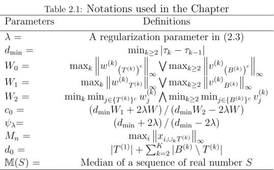
Table 2.1:

Notations used in the Chapter

Parameters

Definitions

λ

=

A regularization parameter in (2.3)

d

=

min

|

τ

−

τ

|

W

=

max

w

(

)

W

max

v

(

)

W

=

max

w

W

max

v

W

=

min

min

w

V

min

min

v

c

=

(d

W

+ 2λW

)

/

(d

W

−

2λW

)

ψ

=

(d

+ 2λ)

/

(d

−

2λ)

M

=

max

x

d

=

|

T

|

+

P

|

B

\

T

|

M

(S

) =

Median of a sequence of real number

S

2.3

Theoretical Properties

We first define the following cone constraint: for any set J ⊂ {1,· · · , p}and any positive number c,

C(J, c) ={x∈_Rp _{|x6= 0, kx}

Jck₁ ≤ckx_Jk₁}.

Define a restricted eigenvalue (RE) condition (Bickel et al., 2009; van de Geer and Buhlmann, 2009): for any integer 0< s < p and any positive numberc > 0, RE(s, c) means k2(s, c) := min J⊆{1,...,p}, |J|≤s min δ∈C(J,c) δT_XT_Xδ nkδJk22 >0, (2.5)

which is imposed on the p×psample covariance matrix XT_{X/n. The RE condition}

is needed to guarantee consistency of the Lasso and Dantzig selectors (Bickel et al., 2009). This condition also implies that the gram matrix XT_{X/n behaves like a}

Similarly, we introduce a restricted nonlinear impact (RNI) condition, as in Bel-loni and Chernozhukov (2011): For any integer 0 < s < p and any positive number

c >0, RNI(s, c) means q(s, c) := min J⊆{1,...,p}, |J|≤s min δ∈C(J,c) kXδk3 2 n1/2_kXδk3 3 >0, (2.6)

which controls the norm kXδk3 bykXδk2 over the cone C(J, c) for any J such that |J| ≤s. RNI(s, c) can be equivalently written as for δ ∈C(J, c),

1 n n X i=1 |xT_i δ|2 !3 ≥q2(s, c) 1 n n X i=1 |xT_i δ|3 !2 ,

which implies that the third sample moment is controlled by the second sample moment. This condition is necessary to control the quantile regression objective function by quadratic terms (Belloni and Chernozhukov, 2011).

Condition 2.3.1. [On the conditional density] For each i = 1, . . . , n, let fi(·)

denote the probability density function of yi given xi. The function fi(·) has a

continuous derivativef_i0(·). For eachi,fi(·)≤f,|fi0(·)| ≤f andminkfi xiTβ(τk)

≥

f for some constants f , f >0.

Condition 2.3.2. [On the weights] Let W0 and W1 be the maximum weight

imposed on the zero components and nonzero components, respectively, and W2 be

the minimum weight imposed on zero components. The weights satisfy

W2

W0∨W1

≥ 2.5λ mink|τk−τk−1|

.

Condition 2.3.3. [On the growth rate of the sparsity] The maximal sparsity s0

Condition 2.3.1 is the same as Condition D.1 in Belloni and Chernozhukov (2011). For the location model and the location-scale model, Belloni and Chernozhukov (2011, Lemmas 1 and 2) analyze the sufficient conditions of Condition 2.3.1 by spec-ifying the values of f,f. Condition 2.3.2 imposes a lower bound onW2/(W0∨W1). This condition implies that W2 must not be too small, which means that zero com-ponents must be penalized in the optimization problem (2.3) and (2.4). In Sections 2.3 and 2.4, we show that W0, W1 and W2 can be constructed from an appropriate initial estimator, and W0 and W1 are upper bounded and W2 is lower bounded by some constants. Condition 2.3.3 is necessary for the consistency of our estimators.

Remark 2.3.1. Note that the regular adaptive lasso weights are used in Jiang et al. (2013), where w_j(k) = 1/|βe (k) j |q and v (k) j = 1/|βe (k) j −βe (k−1)

j |q with an initial estimate

e

β(k) at quantile level τk and q >0. Condition 2.3.2 is not guaranteed for this weight

because W0 ∨W1 can have any arbitrary large number. This motivates us to use a different type of weights, and in Section 3 the derivative of the SCAD penalty function is used for calculating the weightsw_j(k) and v(_jk) that satisfy Condition 2.3.2 with high probability, as can be seen in the proof of Theorem 2.5.1.

Throughout this section, for any η≥0, let _Eη be the event

Eη = ( 0≤rk− 1 n n X i=1 ρτk yi−xi T_β(τ k) ≤η (k = 1, . . . , K) ) . (2.7)

The following theorem shows the consistency of the proposed estimator Bb.

Theorem 2.3.1. Suppose that Conditions 2.3.1-2.3.2,RE(2s0, c0)and RNI(2s0, c0)

hold. Let Bb= [βb(1),· · · ,βb(K)] be the solution to (2.3) and (2.4). Let η_n = o(1) be

any sequence of positive numbers with0≤ηn<9f3q2(2s0, c0)/(32f

2

with probability at least 1−1/n−_P(_Ec ηn), max k k b β(k)−β(τk)k2 ≤ξ1 r s0logp n +ηn, (2.8) K X k=1 kβb (k) {T(k)_}ck1 _ λ K X k=2 {βb(k)−βb(k−1)}_{B(k)_}c |τk−τk−1| 1 ≤ξ3s0K r logp n +ξ3 √ s0K √ ηn, (2.9)

where for some absolute constant C1 >0,

ξ1 = 2(1 +c0)2 k(2s0, c0) p f 1 + 2C1 k(s0, c0) and ξ3 =ξ1 W1 W2 . (2.10)

The upper bound in (2.8) implies that the estimates βb(k) for k = 1,· · ·K_n are

uniformly consistent when ηn =o(1) andn = Ω(s0logp). The upper bound in (2.8) has two components, where the first component ps0logp/n is within a factor of √

logp of the oracle rate, and the second component √ηn characterizes the bias

induced by the use of the feasible regionR(k)_(r

k) in (2.7). To obtain the consistency

rate ps0logp/n for βb(k) in (2.8), which is an expected bound for high dimensional

models (Belloni and Chernozhukov, 2011; Fan et al., 2014a; Zheng et al., 2015),

ηn=O(s0logp/n) is required. By using a consistent initial estimate, we can choose suchηn with rk such that the event Eηn holds with a high probability; See (2.16) for

details.

As can be seen in (2.8), as ηn increases, the estimation error bound is larger while

the probability_P(_Ec

ηn) becomes smaller. The optimalrkis

1 n Pn i=1ρτk yi−xi T_β(τ k) , which provides the fastest convergence rate. Therefore, using rk near this optimal

value in (2.4) is a key part of our implementations. We use a proper initial estimate of β(k) _{to estimate the optimal value r}

Inequality (2.9) shows that the `1 norm of the quantile coefficients estimates for inactive predictors (with true zero coefficients) converges to zero provided that

W1/W2 = o(1), Kn2ηn = o(1) and n = Ω(Kn2s0logp). Moreover, the `1 norm is deceasing as W1/W2 becomes smaller, which implies that choosing smaller weights

W1 and larger weightsW2would improve the rate of convergence, which is consistent with the idea used in adaptive Lasso.

Later in Theorem 2.5.2, we will discuss exact model structure selection by us-ing (2.9) with an additional beta–min condition.

Remark 2.3.2. The quantity ξ1 in (2.10) depends on n by the term k(2s0, c0) and

k(s0, c0). Consider a simple case that τk−τk−1 = 1/Knfor all k, andw

(k)

j =v

(k)

j = 1

for all k and j. Then W0 = W1 = W2 = 1, and Condition 2.3.2 reduces to λ ≤ 2/(5Kn). If λ= 2/(5Kn), then the condition of c0 in Theorem 2.3.1 is equivalent to

c0 ≥9. Specifically, ifc0 = 9, thenξ1 is less than some universal constant given that

k(2s0,9) is lower bounded by some universal constant.

Remark 2.3.3. Our formulation (2.3) enables us to userkas a tunning parameter,

and the scale of rk is more interpretable than a tuning parameter in the Lagrangian

formulation. Letting the weights of the quantile loss functions for all quantile levels to be equal in the dual problem is proposed by Jiang et al. (2013) under the fixed p

setting, which includes fewer regularization parameters. But it is not clear whether model selection consistency holds for such estimators in the high dimensional setting. Moreover, our empirical work shows that, in terms of model selection, our proposed method outperforms the implementation based on the equal weights in the dual problem. See Section 2.7 for details.

2.4

Implementation

We provide a specific realization for the Dantzig–type joint quantile regression in-troduced in Section 2.2. This procedure involves the derivative of the SCAD penalty function (Fan and Li, 2001):

Pζ(x) =I(x≤ζ) +

(3.7ζ−x)+

2.7ζ I(x > ζ)

with a regularization parameter ζ ≥0. We now specify the multi-step procedure.

Step 1. Obtain initial estimates. We obtain initial estimates following Belloni and Chernozhukov (2011). Let eλ= 1.1 Π(0.9) be a regularization parameter, where

Π(0.9) is defined in Remark 2.4.1, e β(k) = arg min β∈Rp 1 n n X i=1 ρτk yi−xi T β+eλkβk1 (k = 1, . . . , Kn). (2.11)

Step 2. Solve the Dantzig-type optimization. To solve the optimization (2.3) and (2.4), we use the following specifications.

Step 2a: For the parameters in the objective function (2.3), we use the following specifications. Let _es = maxkkβe(k)k₀.

ζn= 0.1 p e slogp/n, (2.12) w(_jk) =Pζn |βe (k) j | (k = 1, . . . , Kn), (2.13) v(_jk) =Pζn |βe (k) j −βe (k−1) j | (k = 2, . . . , Kn), (2.14) λ= 0.4 min k≥2 |τk−τk−1|. (2.15)

Step 2b Let h >0 denote a scaling parameter to be chosen and Λ(_kh) ≥0 (k = 1, . . . , Kn) be regularization parameters taken to be Λ

(h)

defined in Table 1 and Rk =

n

|yi−xiTβe(k)|:i= 1, . . . , n o

. For the parameter rk

in the constraint (2.4), we use

r(_kh)= 1 n n X i=1 ρτk yi−xiTβe(k) + Λ(_kh)eslogp n (k = 1, . . . , Kn). (2.16) Step 3. Choose h. We use 5-fold cross validation to minimize the sum of the quantile loss functions over all quantiles of interest. More specifically, we ran-domly split the data into five roughly equal parts X(1)_{,· · · , X}(5) _∈

R[n/5]×p and

y(1)_{,· · · , y}(5) _∈

R[n/5]×1, respectively. For t = 1,· · · ,5, let X(t) =

h

x₁(t),· · · , x_[(_n/t)_5]iT. Let βb

(k)

t (h) (k = 1,· · · , Kn) be the solution to the (2.3) and (2.4) following Step 1

and Step 2 for the data X and Y excluding the tth fold. Let the CV score function

score(h) := 5 X t=1 Kn X k=1 [n/5] X i=1 ρτk y_i(t)−(x(_it))Tβb (k) t (h) .

We chooseh0 from the setS :={0.01,0.02,· · · ,4} that minimizes the score, that is,

ho := arg min

h∈S

score(h).

The Dantzig-type estimate βb(k) is the solution to (2.3) and (2.4) using the

afore-mentioned specifications withh=ho, Λk := Λ

(ho₎

k , andrk :=r

(h0₎

k .

In Step 2 (b), Λ(_kh) plays the role of scaling to achieve scale equivariance of the method. It is obvious that those choices of the regularization parameters do not give the best results for any given models, but they lead to good empirical results in a variety of settings and could help understand how the proposed Dantzig–type penalization performs with reasonable choices of these tuning parameters.

Remark 2.4.1. Following Belloni and Chernozhukov (2011), define

Π := max 1≤k≤Kn max 1≤j≤p 1 n n X i=1 xij(τk−I(ui ≤τk)) p τk(1−τk) ,

whereu1,· · · , unare independent and identically distributed from the uniform

distri-bution on (0,1) and independent of xis, and xij is the jth component of the design

xi for i = 1, . . . , n and j = 1, . . . , p. Let Π(0.9) be the 0.9th quantile of Π that

can be computed using simulated Π. As seen in Step 1, we use eλ = 1.1 Π(0.9),

where the constant factor 1.1 differs from the recommendation made in Belloni and Chernozhukov (2011), giving us initial estimates with low false negative rates.

2.5

Theoretical Properties (continued)

LetBb= [βb(1),· · · ,βb(Kn)] be any optimum of (2.3) and (2.4), wherew

(k)

j s,v

(k)

j s and

rks are defined in (2.13), (2.14) and (2.16). Define an event for the initial estimates

e

β(k)s for k = 1, . . . , Kn as follows: for some positive constantsC2, C3 and C4,

E1 = ( e λ≤C2 r logp n , maxk kβe (k)₋ β(τk)k2 ≤C3 r s0logp n , maxk kβe (k)_k 0 ≤C4s0 ) , (2.17) Denote byγn:=P(E1c) the probability that the event E1 does not occur.

Belloni and Chernozhukov (2011) prove that their estimators and the correspond-ing regularization parameters as stated in (2.11) satisfy conditionE1with probability close to 1.

For theoretical properties of the estimates detailed in Section 2.4, we assume the following conditions.

Condition 2.5.1. [On the regularization parameters] Assume that

min k Λk ≥6 p C4+ 1C3 and ζn ≥2C3 p s0logp/n.

Condition 2.5.2. [On the non-zero coefficients] The following beta-min conditions

hold for some positive constants C5 and C6,

min k jmin∈T(k)|βj(τk)| > C5 r s0logp n , (2.18) min k≥2 _jmin∈B(k) |βj(τk)−βj(τk−1)| |τk−τk−1| > C6Kn r s0logp n , (2.19)

where we assume n = Ω(K2s0logp).

Our multi-step Dantzig–type joint quantile estimator Bbis consistent as shown in

the following theorems.

Theorem 2.5.1. Suppose Conditions 2.3.1,2.3.3,2.5.1,RE(2s0, ψλ)andRNI(2s0, ψλ)

hold. Then with probability at least 1−2/n−γn, Bbsatisfies

max k k b β(k)−β(τk)k2 ≤ξ2 r s0logp n ,

where for some absolute constant C >0, ξ2 = _k(2s C

0,ψλ)

√

f

√

1 + maxkΛk.

The following Theorem 2.5.2 shows that Bb recovers the exact model structure

under appropriate conditions.

Theorem 2.5.2. Suppose that the conditions of Theorem 2.5.1 and Condition 2.5.2 hold. Then

P

n b

T(k) =T(k) and Bb(k) =B(k) for all k o

≥1− 2

n −γn.

Theorem 2.5.1 follows from (2.8) in Theorem 2.3.1 and shows that our multi-step Dantzig–type joint quantile estimator Bb is consistent when n = Ω(s0logp) under appropriate conditions. Theorem 2.5.1 requires the lower bound of Λkfor the feasible

regions (2.4) to include the true parameter Bo _{with high probability. In simulations,}

our estimator still worked quite well even if Λk is set to zero so Condition 2.5.1 is

violated.

Theorem 2.5.2 implies that the true parameter Bo _{belongs to the set of optimal}

solutions with high probability and Bb recovers the true model structure with high

probability, which also satisfies the exact model selection property (Zhao and Yu, 2006; Wainwright, M., 2009; Fan et al., 2014a).

Remark 2.5.1. The beta-min condition (2.18) imposes a lower bound of the nonzero coefficients. While Condition (2.18) has been studied in high dimensional analysis to establish the exact model selection property (Meinshausen and B¨uhlmann, 2006; van de Geer et al., 2011; B¨uhlmann and van de Geer, 2011), the beta-min condition (nonzero rate of change in interquantile coefficients) that provides a lower bound on the nonzero interquantile differences rate has not been considered elsewhere.

The beta–min condition (2.19) can be demonstrated by the following example. For simplicity, we consider equally-spaced quantile levels τk (k = 1, . . . , Kn) with

τk−τk−1 1/Kn. Consider a location–scale model, as used in Example 2.7.2 in

Section 2.7, yi = xiTβ +xiTri, where the design xi and the vector r ∈ Rp have

nonnegative components with xT

i r > 0 for all i. Then (2.19) holds as long as the

components of r satisfyrj1{rj 6= 0} Kn

p

s0logp/n (j = 1, . . . , p), where rj is the

jth component of r.

2.6

Post–Selection Joint Quantile Regression

We consider a post–selection joint quantile regression that minimizes the sum of quantile loss functions over all quantiles of interest based on the model

struc-ture Tb(k) (k = 1, . . . , Kn) and Bb(k) (k = 2, . . . , Kn) of the multi-step Dantzig–type

joint quantile estimator Bb= [βb(1),· · · ,βb(K)] as described in Section 2.4. The post–

selection joint quantile estimator (POST JQR) denoted byBbpo is a minimizer of

min B=[β(1)_,···,β(Kn)_]∈G X k X i ρτk yi−xi T_β(k) , where (2.20) G=nB= [β(1), . . . , β(Kn)_]∈ Rp×Kn :β(k){Tb(k)}c = 0, β (k) {Bb(k)}c =β (k−1) {Bb(k)}c o

is a set of matrices whose induced model structure is the same as the structure of Bb. Throughout this section, we assume that Tb(k) = T(k) (k = 1, . . . , K_n) and

b

B(k) =B(k) (k = 2, . . . , Kn), which holds with probability tending to 1. As can be

seen in the proof of Theorem 2.6.1 in the Supplementary material, there is a one-to-one mapping T between G and _Rd0_{, where d}

0 is the effective dimension of the parameter for the selected model as defined in Table 4.1. In other words, the set

G ⊂ _Rp×Kn _{in (2.20) can be embedded in}

Rd0. We use T(Bbpo) to estimate T(Bo),

which is a d0–dimensional vector that consists of the active components ofBo_.

To establish the theoretical properties of T(Bbpo), we redefine POST JQR. As

defined in the proof of Theorem 2.6.1 in the Supplementary material, there exist new design variables z_i(k) (i= 1, . . . , n; k= 1, . . . , Kn) such that

T(Bbpo) = arg min β∈Rd0 X k X i ρτk yi−(z (k) i ) T_{β. (2.21)}

Now to establish the asymptotic convergence rate and asymptotic normality of

T(Bbpo), we use the following sparse eigenvalue condition: For 0< s < p,

Sparse(s) : φ(s) = max kδk0≤s kXδk2 2 nkδk2 2 <∞. (2.22)

Sparse(s) means that the maximal s-sparse eigenvalue of the gram matrix XT_X/n

et al., 2015). We use the following conditions to show the theoretical properties of the estimator.

Condition 2.6.1(a). [On the sample size]

n= Ω d0s30(logn) 6_∨M4 nd0(logn)2 . Condition 2.6.1(b). n= Ω (d5 0s30(logn)6∨Mn2d30s0).

Condition 2.6.1(a) is used to show the asymptotic oracle consistency of the estima-tor in Theorem 2.6.1, and Condition 2.6.1(b) is required for showing the asymptotic normality of the estimator in Theorem 2.6.2. These conditions involve d0, s0, Mn

and n. If the entries in xi are uniformly bounded, and d0 and s0 grow slowly with

n, Condition 2.6.1(a) is quite mild. The POST JQR enjoys the asymptotic oracle consistency rate as follows:

Theorem 2.6.1. Suppose the conditions of Theorem 2.5.2 together with Condition

2.6.1(a) and Sparse(s0). Then

kT(Bbpo)−T(Bo)k2 =Op

p

d0/n

. (2.23)

Theorem 2.6.2. Suppose that the conditions of Theorem 2.6.1 and Condition

2.6.1(b) hold. Then, for any sequence of vectors αn ∈Rd0 with kαnk2 = 1,T(Bbpo) is

asymptotically normal, α_nT√n(An−1BnAn−1)− 1 2 T(Bbpo)−T(Bo) →d_N(0,1), where An= Kn X k=1 n X i=1 1 nfi xi T_β(τ k) z_i(k)z_i(k) T ,

Bn= n X i=1 X k,k0_=1,...,K n 1 nz (k) i z(_ik0) T (τk∧τk0 −τ_kτ_k0),

with z_i(k) given in the proof of Theorem 2.6.1 in the Supplementary material.

Theorem 2.6.2 provides sufficient conditions for the asymptotic normality of POST JQR, which relies on the exact model structure property as defined in Theo-rem 2.5.2. This property is typically fragile without beta-min condition, and is not uniformly valid (Leeb and P¨otscher, 2005). Leeb and P¨otscher (2003) and Belloni et al. (2015) considered the post-model-selection estimator conditional on selecting an incorrect model, and established the uniform asymptotic distribution of the esti-mator. Establishing an asymptotic distribution without beta-min condition in our setting will also be of interest in a follow-up work.

2.7

Numerical Studies

Our optimization problem (2.3) is equivalent to a linear programming problem with the aid of slack variables, and can be solved by existing optimization packages in a way that is similar to the problem of Jiang et al. (2013). For the other estimators, we useβe(k) as an initial estimate at τ_k-th quantile. More specifically, ALasso atτ_k is

arg min β∈_Rp 1 n n X i=1 ρτk(yi−xi T_{β) +λ} ad,k p X j=1 |βj|/|βe (k) j |,

whereλad,k is the regularization parameter to be chosen by 5-fold cross validation to

minimize the τk-th quantile loss function, and FAL (Jiang et al., 2013) finds

arg min [β(1)_,···,β(Kn)_]∈ Rp×K 1 n Kn X k=1 n X i=1 ρτk yi−xi T β(k) + λa Kn X k=1 p X j=1 w(_jk)|β_j(k)|+ Kn X k=2 p X j=1 v_j(k)|β_j(k)−β_j(k−1)| ! ,

where w_j(k) = 1/|βe (k) j | and v(k)j = 1/|βe (k) j − βe (k−1)

j | and λa is the regularization

parameter to be chosen by 5-fold cross validation to minimize the sum of quantile loss functions over all quantiles of interest. Our proposed estimator Dantzig is described in Section 2.4.

To assess the performances of the competing methods, the following performance measures were calculated based on 100 Monte Carlo replications.

1. “F Pk”, the number of false positives in the selected model atτk, i.e.,|Tb(k)\T(k)|;

2. “F Nk”, the number of false negatives in the selected model atτk, i.e.,|T(k)\Tb(k)|;

3. “SDk”, the size of the set difference of the selected models for adjacent quantile

levels, τk and τk−1, i.e.,|Tb(k)4Tb(k−1)| for k = 2, . . . , K_n;

4. “F PU”, the number of false positives in the union of the selected models across

all quantile levels, i.e., | ∪kTb(k)\ ∪_kT(k)|;

5. “F NU”, the number of false negatives in the union of the selected models across

all quantile levels, i.e., | ∪kT(k)\ ∪kTb(k)|.

In the following examples, we consider five different models, a location model, a location-scale model and a random coefficient model.

Example 2.7.1. Consider the linear regression model with(n, p, Kn, s0) = (100,500,5,6)

and (τ1, τ2, τ3, τ4, τ5) = (0.30,0.40,0.50,0.60,0.70):

yi =xiTβ+i, β = (1.0,0.8,0.0,0.9,0.5,0.0,0.3,0.7,0.0,· · · ,0.0)T,

whereis are independent and identically distributed from the standard normal

is generated from the autoregressive model, AR(1), with correlation 0.5, that is,

Σ(i,j) = 0.5|i−j|.

Example 2.7.2. Consider the following location-scale model with (n, p, Kn, s0) =

(100,500,5,7)and (τ1, τ2, τ3, τ4, τ5) = (0.30,0.40,0.50,0.60,0.70):

yi =x1+ 0.8x2 + 0.9x4+ 0.5x5+ 0.3x7+ 0.75x8+ (0.5x2+x3 + 0.5x8)i,

whereis are independent and identically distributed from the standard normal

dis-tribution and independent ofxis. The regressors are generated in two steps, following

Wang et al. (2012). First generate _exij ∼N(0,Σx) from the AR(1) model, with

cor-relation0.5, and then xij = Φ(xeij) (j = 2,3,8)and xij =xeij (j 6= 2,3,8), where Φis

the cumulative distribution function of the standard normal distribution.

Example 2.7.3. Consider the random coefficient model with(n, p, Kn, s0) = (100,500,5,6)

and (τ1, τ2, τ3, τ4, τ5) = (0.70,0.75,0.80,0.85,0.90):

yi =xiTβ(ui), β(ui) = (β1(ui),· · · , βp(ui))T,

where u1,· · · , un are independent and identically distributed from the uniform

dis-tribution on (0,1) and independent of xi, and β1(u) = 1.7 + Φ−1(u), β2(u) = 0.35,

β3(u) = 3(u−0.8)+, β5(u) = 0.5 + 0.5×2u, β6(u) = 0.5 +u,β10(u) = 0.4 + √

uand

βj(u) = 0 (j 6= 1,2,3,5,6,10). The regressors are generated in the same way as in Example 2.7.2.

Example 2.7.4. Consider the model, which is same as Example 1 in the main

paper except thatis follow the standard Cauchy distribution.

Example 2.7.5. Consider the model, which is same as Example 1 in the main

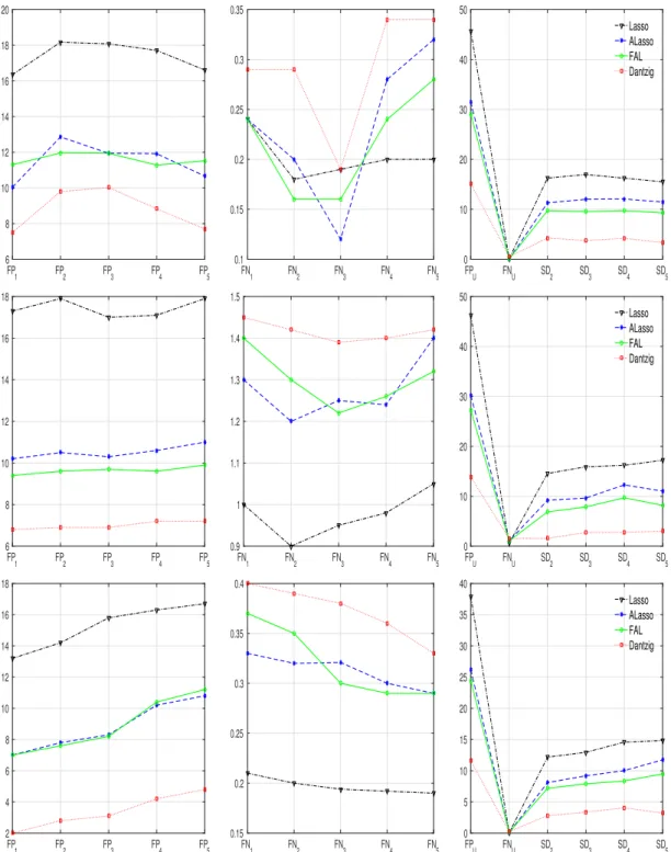
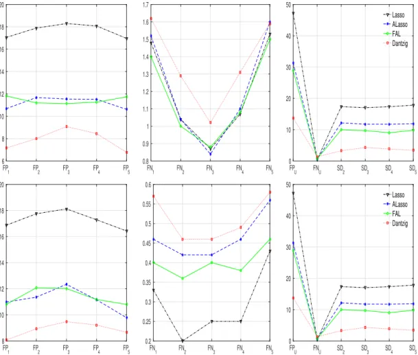
Figure 2.1 shows the performance measures defined in Subsection 2.7.1 for Exam-ples 2.7.1–2.7.3. The first, second and third rows correspond to Example 2.7.1, Ex-ample 2.7.2 and ExEx-ample 2.7.3, respectively. Each row consists of three sub-figures. The first and the second sub-figures show the number of false positives and the num-ber of false negatives for each of the five quantile levels, respectively, which explains the quality and the sparsity of the selected models. The last sub-figure shows the size of the set differences of the selected models at adjacent quantile levels, and the number of false positives and false negatives of the union of the selected covariates over the five quantile levels, which explains the stability of the model. Across all figures, the largest standard errors for the false positives, the false negatives and the size of set differences are less than 0.9, 0.1 and 0.5, respectively.

As seen in Figures 2.1 and 2.2, Dantzig includes smaller number of false positives with more false negatives compared to the other methods. But this increase in false negatives is relatively small considering the decrease in false positives. Dantzig has a smaller size of set difference for two neighboring quantiles, and fewer false positives than other methods for the union of the selected variables across the five quantile levels. This indicates that Dantzig shares many common variables across different quantiles, and provides more stable models. Overall, at each quantile, Dantzig provides sparser model than other competitors in all the examples. In terms of stability of the selected models across quantiles, Dantzig outperforms the others.

FP 1 FP2 FP3 FP4 FP5 6 8 10 12 14 16 18 20 FN 1 FN2 FN3 FN4 FN5 0.1 0.15 0.2 0.25 0.3 0.35 FP_U FN_U SD₂ SD₃ SD₄ SD₅ 0 10 20 30 40 50 Lasso ALasso FAL Dantzig FP 1 FP2 FP3 FP4 FP5 6 8 10 12 14 16 18 FN 1 FN2 FN3 FN4 FN5 0.9 1 1.1 1.2 1.3 1.4 1.5 FP_U FN_U SD₂ SD₃ SD₄ SD₅ 0 10 20 30 40 50 Lasso ALasso FAL Dantzig FP 1 FP2 FP3 FP4 FP5 2 4 6 8 10 12 14 16 18 FN 1 FN2 FN3 FN4 FN5 0.15 0.2 0.25 0.3 0.35 0.4 FP_U FN_U SD₂ SD₃ SD₄ SD₅ 0 5 10 15 20 25 30 35 40 Lasso ALasso FAL Dantzig

Figure 2.1: Results for Example 2.7.1 (top), 2.7.2 (middle) and 2.7.3 (below): Include false positives(left), false negatives (middle) and the stability measures (right). Four competing procedures are evaluated: Lasso, ALasso, FAL and Dantzig.

FP 1 FP2 FP3 FP4 FP5 6 8 10 12 14 16 18 20 FN 1 FN2 FN3 FN4 FN5 0.8 0.9 1 1.1 1.2 1.3 1.4 1.5 1.6 1.7 FP_U FN_U SD₂ SD₃ SD₄ SD₅ 0 10 20 30 40 50 Lasso ALasso FAL Dantzig FP 1 FP2 FP3 FP4 FP5 8 10 12 14 16 18 20 FN 1 FN2 FN3 FN4 FN5 0.2 0.25 0.3 0.35 0.4 0.45 0.5 0.55 0.6 FP_U FN_U SD₂ SD₃ SD₄ SD₅ 0 10 20 30 40 50 Lasso ALasso FAL Dantzig

Figure 2.2: Results for Example 2.7.4 (top) and 2.7.5 (below): Include false positives (left), false negatives (middle) and the stability measures (right). Four competing procedures are evaluated: Lasso, ALasso, FAL and Dantzig.

2.8

Application

We consider the proposed Dantzig–type joint quantile regression method in an application to a genetic data set used in Scheetz et al. (2006). This data set consists of the expression values of 31042 probe sets for 120 rats. As in Huang et al. (2008), Kim et al. (2008) and Wang et al. (2012), we are interested in finding genes that are related to gene TRIM32, which is known for causing Bardet-Biedl syndrome.

The model selection approach is applied to 300 probe sets that pass an initial screening. See Huang et al. (2008) for details of the screening steps. We apply

Dantzig, Lasso, ALasso and FAL, which are defined in Section 2.7, and SCAD (Wang et al., 2012) on these 300 probe sets (p= 300) with 120 rats (n = 120). SCAD is a single quantile regression method, which uses the SCAD penalty function to penalize quantile coefficients. We consider two sets of five quantile levels (τ1, τ2, τ3, τ4, τ5) as (0.48,0.49,0.50,0.51,0.52) and (0.81,0.82,0.83,0.84,0.85), representing interests in the middle and the upper tail of the distribution of the target gene expressions. To select a tuning parameter for each method, we use 5-fold cross validation. See Subsections 2.4.1 and 2.7.1 for details.

We report the number of nonzero coefficients (“SIZ”) selected by each method at each quantile level. The size of the set difference of the selected models at ad-jacent quantile levels (“DIF”) and the size of the union of the selected covariates over five quantile levels (“TOT”) are considered to investigate the stability of the selected models. As can be seen in Table 2.2, the Dantzig–type estimators, Dantzig and Dantzig0, consistently provide sparser model than other methods. Dantzig also provides the most stable model as we expected.

We also randomly divide the data set into a training set and a test set; the training set includes 80 rats and the test set includes 40 rats. We estimate the models with each method, by using the training set, and record “SIZ”, “DIF” and “TOT”. The prediction error (“PRE”) is calculated over the test set as the quantile loss for each quantile level τk. We repeat this random experiments 100 times and report the

average value of “SIZ”, “DIF”, “TOT” and “PRE” over the 100 repetitions for each method in Table 2.3. As seen in Table 2.3, all of the six methods are similar in terms of prediction error. In terms of the sparsity of the selected models, all of the methods except Lasso are similar. But in terms of the stability of models, Dantzig

outperforms other competitors as we expected. In Table 2.3, the largest standard errors for the columns corresponding to SIZ, DIF, PRE and TOT are less than 0.7, 0.3, 0.05 and 1.2, respectively.

Table 2.2:

Performance results of whole dataset

Method SIZ DIF TOT Method SIZ DIF TOT

Lasso (0.48) 37 Lasso (0.81) 37 Lasso (0.49) 38 9 Lasso (0.82) 41 8 Lasso (0.50) 35 15 Lasso (0.83) 39 8 Lasso (0.51) 36 5 Lasso(0.84) 36 7 Lasso (0.52) 37 3 45 Lasso (0.85) 38 4 49 SCAD (0.48) 24 SCAD (0.81) 20 SCAD (0.49) 24 0 SCAD (0.82) 25 9 SCAD (0.50) 20 6 SCAD (0.83) 16 9 SCAD (0.51) 14 7 SCAD (0.84) 29 13 SCAD (0.52) 18 5 25 SCAD (0.85) 27 4 35 ALasso (0.48) 27 ALasso (0.81) 25 ALasso (0.49) 17 14 ALasso (0.82) 24 3 ALasso (0.50) 20 7 ALasso (0.83) 22 4 ALasso (0.51) 14 6 ALasso (0.84) 21 3 ALasso (0.52) 15 1 29 ALasso (0.85) 28 7 34 FAL (0.48) 21 FAL (0.81) 25 FAL (0.49) 21 0 FAL (0.82) 25 1 FAL (0.50) 22 2 FAL (0.83) 26 2 FAL (0.51) 21 3 FAL (0.84) 25 2 FAL (0.52) 21 2 25 FAL (0.85) 25 2 26 Dantzig (0.48) 21 Dantzig (0.81) 21 Dantzig (0.49) 19 2 Dantzig (0.82) 20 1 Dantzig (0.50) 20 1 Dantzig (0.83) 21 1 Dantzig (0.51) 21 3 Dantzig (0.84) 22 2 Dantzig (0.52) 20 1 22 Dantzig (0.85) 21 1 24

Table 2.3:

Performance results of 100 random partitions of the data

Method SIZ DIF PRE TOT Method SIZ DIF PRE TOT

Lasso (0.48) 30.94 1.79 Lasso (0.81) 32.94 1.33 Lasso (0.49) 31.10 3.35 1.79 Lasso (0.82) 33.04 4.22 1.30 Lasso (0.50) 31.76 4.38 1.78 Lasso (0.83) 33.00 6.36 1.26 Lasso (0.51) 31.92 4.66 1.78 Lasso (0.84) 32.88 4.20 1.23 Lasso (0.52) 32.60 4.78 1.78 37.73 Lasso (0.85) 32.78 4.34 1.21 40.28 SCAD (0.48) 22.04 1.79 SCAD (0.81) 20.90 1.32 SCAD (0.49) 22.82 5.10 1.78 SCAD (0.82) 20.32 6.46 1.27 SCAD (0.50) 21.86 5.44 1.78 SCAD (0.83) 21.02 6.62 1.27 SCAD (0.51) 21.38 4.52 1.78 SCAD (0.84) 22.10 6.12 1.23 SCAD (0.52) 21.66 5.40 1.79 28.74 SCAD (0.85) 20.50 5.16 1.20 28.86 ALasso (0.48) 19.96 1.82 ALasso (0.81) 19.98 1.34 ALasso (0.49) 19.70 2.98 1.79 ALasso (0.82) 19.22 4.04 1.31 ALasso (0.50) 19.32 3.46 1.80 ALasso (0.83) 20.04 5.34 1.26 ALasso (0.51) 19.08 3.40 1.80 ALasso (0.84) 19.92 3.36 1.25 ALasso (0.52) 19.64 3.76 1.80 24.56 ALasso (0.85) 19.44 3.60 1.21 25.78 FAL (0.48) 19.75 1.85 FAL (0.81) 20.95 1.37 FAL (0.49) 20.70 1.28 1.82 FAL (0.82) 21.71 2.34 1.32 FAL (0.50) 20.72 1.94 1.88 FAL (0.83) 20.33 3.90 1.27 FAL (0.51) 20.18 2.40 1.82 FAL (0.84) 20.18 2.76 1.25 FAL (0.52) 19.94 2.59 1.83 23.63 FAL (0.85) 21.74 2.20 1.22 24.55 Dantzig (0.48) 20.20 1.84 Dantzig (0.81) 21.94 1.33 Dantzig (0.49) 20.06 0.98 1.84 Dantzig (0.82) 21.72 1.02 1.31 Dantzig (0.50) 19.98 1.82 1.82 Dantzig (0.83) 21.98 2.70 1.27 Dantzig (0.51) 20.70 2.01 1.81 Dantzig (0.84) 21.60 1.78 1.25 Dantzig (0.52) 21.02 2.52 1.80 22.90 Dantzig (0.85) 21.42 1.18 1.22 23.86

2.9

Conclusion

Model selection stability across quantile levels adds credibility and interpretabil-ity of the selected models in applications. If the selected models vary significantly from one quantile to the next when the quantile levels used are very close to each other, it could be an undesirable feature of model selection. The proposed Dantzig– type approach leads to a much more stable selection without a noticeable sacrifice on the prediction error. We adopt a Dantzig–type optimization problem and es-tablish the uniform non-asymptotic error bounds and model selection consistency

under appropriate conditions. By using the selected model structure, we also study post–selection joint quantile regression and establish its asymptotic distributions. The simulation study and real data analysis show that the proposed method consis-tently provides sparse and stable models, and reduces the noisy component in model selection at single quantile levels for both homogeneous and heterogeneous cases.

2.10

Supplementary Material

Let Fi denote the conditional distribution of yi given xi for i = 1, . . . , n, that is

Fi(x) = P[yi ≤x|xi] for all x∈R. Define the diagonal matrices

Hk= diag f1 x1Tβ(τk) ,· · · , fn xnTβ(τk) (k = 1, . . . , Kn),

where f1,· · · , fn are defined in Condition 2.3.1 of the main paper. Then for any

vector δ∈_Rp_{, we define an intrinsic norm as in Belloni and Chernozhukov (2011),}

kδkk,2 = r δTX T_H kX n δ (k = 1, . . . , Kn). (2.24)

For any positive constantc and the sets T(k) _{(k= 1, . . . , K}

n) defined in (2.2), let

A(k)(c) =δ:δ 6= 0, δ∈_Rp_{, kδ}

{T(k)_}ck₁ ≤ckδ_T(k)k₁ .

Define the function as follows: for k= 1, . . . , Kn,

Q(nk)(β) = 1 n n X i=1 ρτk(yi−xi T β),

where the subdifferential of _Q(nk)(β) at β is the following set of vectors (Wang et al.,

2012): ∂_Q(_nk)(β) = ( δ ∈_Rp _|δ j =− τ n X i xijI(yi > xiTβ) + 1−τ n X i xijI(yi < xiTβ)− 1 n X i xijvi ) ,

where xij is the jth component of xi, and vi = 0 if yi =6 xiTβ and vi ∈ [τ −1, τ]

otherwise. For simplicity, for any B= [β(1)_{,· · · , β}(K)_]∈

Rp×Kn, let G(B) = Kn X k=1 p X j=1 w_j(k)|β_j(k)|+λ Kn X k=2 1 |τk−τk−1| p X j=1 v_j(k)|β_j(k)−β_j(k−1)|, (2.25)

which is the objective function of our optimization problem as defined in (2.3), where

w(k) _{(k = 1, . . . , K}

n) and v(k) (k = 2, . . . , Kn) are p-dimensional wight vectors.

For any square matrix A, let λmax(A) and λmin(A) be the maximum eigenvalue and the minimum eigenvalue of A, respectively.

Preliminary Results

The following Lemma 2.10.1 controls the empirical error over all vectors inA(k)(c0) for all k= 1, . . . , Kn and is analogous to Lemma 5 of the Belloni and Chernozhukov

(2011).

Lemma 2.10.1. Let c0 and t1,· · · , tKn be positive numbers. Suppose Condition

2.3.1 and RE(2s0, c0) hold. Let

e

Q(k)(v) = EQ(nk){β(τk) +v} −Q(nk){β(τk)}

−_Q(k)

n {β(τk) +v}+Qn(k){β(τk)}.

for any v ∈_Rp_{. Then we have}

P ( sup v∈A(k)_(c 0),kvkk,2≤tk Qe (k)_(v) > C1 1 +c0 k(s0, c0) tk r s0logp n (k = 1, . . . , Kn) ) ≤ 1 n (2.26)

for some absolute constant C1 >0.

Proof of Theorem 2.3.1

Lemma 2.10.2. Letc0 be a positive number. Suppose RE(2s0, c0)holds. Then we

have for all k= 1, . . . , Kn,

kδk1 ≤ √ s0 1 +c0 p f k(s0, c0) kδkk,2, kδk2 ≤ 1 +c0 p f k(2s0, c0) kδkk,2 for all δ ∈A(k)_(c 0).

The following Lemma 2.10.3 is a fixed design version of (3.7) in Belloni and Chernozhukov (2011), which provides the lower bound of the difference of the ex-pected values of quantile loss function over all vectors in the cone A(k)_(c

0) for all

k = 1, . . . , Kn.

Lemma 2.10.3. Letc0be a positive number. Suppose Condition 2.3.1 and RNI(2s0, c0)

hold. Then we have for all k = 1, . . . , Kn,

E_Q(_nk){β(τk) +δ} −Q(nk){β(τk)} ≥ 3f 3/2 q(2s0, c0) 8 ¯f kδkk,2∧ 1 4kδk 2 k,2 (2.27) for all δ ∈A(k)(c0).

The following Lemma 2.10.4 shows that βb(k) −β(τ_k) is included in the specific

cone for all k.

Lemma 2.10.4. Letηbe any positive number. Let[βb(1),· · · ,βb(Kn)]be an optimum

of (2.3) and (2.4) in the main paper. Suppose Condition 2.3.2 holds. Then on event

Eη defined in (2.7) in the main paper, we have

b β(k)−β(τk)∈A(k) dminW1+ 2λ(W0∨W1) dminW2−2λ(W0∨W1) (k = 1, . . . , Kn),

We fix any c0 and η, which satisfy the conditions in Theorem 2.3.1. Let δk =

b

β(k)_−β(τ

k) (k = 1, . . . , Kn). Let E2 be the event sup v∈A(k)_(c 0),kvkk,2≤kδkkk,2 Qe (k) (v) ≤C1 1 +c0 k(s0, c0) kδkkk,2 r s0logp n (k = 1, . . . , Kn),

where C1 is the constant used in Lemma 2.10.1 and P(E2) ≥ 1−1/n by Lemma 2.10.1.

Proof of (5) in Theorem 2.3.1. Throughout the proof, we assume E2 ∩ Eηn holds.

Lemma 2.10.4 implies that δk is in A(k)(c0) for k = 1, . . . , Kn. By Lemma 2.10.3, we

have that for k = 1, . . . , Kn,

kδkk2k,2 4 ∧ 3f3/2q(2s0, c0) 8 ¯f kδkkk,2 ≤ _Q(k){βb(k)} −Q(k){β(τ_k)} = _Q(_nk){βb(k)} −Q(_nk){β(τ_k)}+ [Q(k){βb(k)} −Q(k){β(τ_k)} −Q(_nk){βb(k)}+Q_n(k){β(τ_k)}] ≤ ηn+ [Q(k){βb(k)} −Q(k){β(τk)} −Q(nk){βb(k)}+Q(_nk){β(τk)}] ≤ ηn+C1 1 +c0 k(s0, c0) r s0logp n kδkkk,2, (2.28)

where C1 is the absolute constant stated in Lemma 2.10.1.

Notice that (2.28) implies that the first term in the left hand side must be less than the second term. Suppose otherwise, that is, kδkkk,2 ≥ 3f3/2q(2s0, c0)/(2 ¯f). Then we have 3f3/2q(2s0, c0) 8 ¯f kδkkk,2 ≤ηn+C1 1 +c0 k(s0, c0) r s0logp n kδkkk,2,

which contradicts the assumption that 0 ≤ ηn < 9f3q2(2s0, c0)/(32 ¯f2), Thus, we conclude kδkk2k,2 4 ≤η+C1 1 +c0 k(s0, c0) r s0logp n kδkkk,2 (k = 1, . . . , Kn),

which yields kδkkk,2 ≤4C1 1 +c0 k(s0, c0) r s0logp n + 2 √ ηn (k= 1, . . . , Kn). (2.29)

By Lemma 2.10.2 and (2.29), we have

kδkk2 ≤4C1 (1 +c0)2 k(2s0, c0)k(s0, c0) p f r s0logp n + 2 1 +c0 k(2s0, c0) p f √ ηn (k = 1, . . . , Kn), which implies kβb(k)−β(τ_k)k₂ ≤ (1 +c0)2 k(2s0, c0) p f 2 + 4C1 k(s0, c0) r s0logp n +ηn=ξ1 r s0logp n +ηn, (2.30) where ξ1 = (1 +c0)2 k(2s0, c0) p f 2 + 4C1 k(s0, c0) .

This completes the proof.

Proof of (2.8) in Theorem 2.3.1. Throughout the proof, we assume E2∩Eηn holds.

The main idea is to compare the objective functions of our optimization problem as stated in (2.3) at Bb and Bo. Since Bo is feasible, G(Bb) must not be greater than

G(Bo_{), where the function G(·) is defined in (2.25). So we have}

0 ≤ G(Bo)−G(Bb) = K X k=1 X j∈T(k) w_j(k)|βj(τk)|+ K X k=2 λ |τk−τk−1| X j∈B(k) v(_jk)|βj(τk)−βj(τk−1)| − Kn X k=1 X j∈T(k) w(_jk)|βb (k) j |+ Kn X k=2 λ |τk−τk−1| X j∈B(k) v(_jk)|βb (k) j −βb (k−1) j |+ Kn X k=1 X j∈{T(k)_}c w_j(k)|βb (k) j | + Kn X k=2 λ |τk−τk−1| X j∈{B(k)_}c v_j(k)|βb (k) j −βb (k−1) j |.

implies Kn X k=1 X j∈{T(k)_}c w(_jk)|βb (k) j |+ Kn X k=2 λ |τk−τk−1| X j∈{B(k)_}c v_j(k)|βb (k) j −βb (k−1) j | ≤ Kn X k=1 X j∈T(k) w_j(k)|βb (k) j −βj(τk)|+ Kn X k=2 λ |τk−τk−1| X j∈B(k) v_j(k)|βb (k) j −βb (k−1) j −βj(τk) +βj(τk−1)| ≤ W1 Kn X k=1 k{βb(k)−β(τ_k)}_T(k)k₁+W₁ Kn X k=2 λ |τk−τk−1| k{βb(k)−β(τ_k)}_B(k)k₁ +W1 Kn X k=2 λ |τk−τk−1| k{βb(k−1)−β(τ_k−1)}B(k)k₁ ≤ W1 p Kn √ s0 v u u t Kn X k=1 k{βb(k)−β(τ_k)}k2₂ (2.31) + 2W1 λ mink≥2|τk−τk−1| p Kn √ 2s0 v u u t Kn X k=1 k{βb(k)−β(τ_k)}k2₂ ≤ ξ1(W1+ √ 2W1) √ s0Kn r s0logp n +ηn, (2.32)

where the third inequality comes from the Cauchy-Schwarz inequality with|T(k)_{| ≤s} 0 and |B(k)_{| ≤2s}

0. Applying (2.32) and the definition of W2, we complete the proof.

Proofs of Theorem 2.5.1

We begin by providing the following lemmas that will be used for the proof of Theorem 2.5.1. Lemma 2.10.5 is only used to show Lemma 2.10.6.

Lemma 2.10.5. For ann×pdesign matrixX = (x1,· · · , xn)T, which is normalized

to have column`2 norm

√

n, we have with probability at least 1−1/n,

max k n X i=1 xi[τk−I{yi ≤xiTβ(τk)}]/n ∞≤3 r logp n . (2.33)

Recall on event E1 defined in (2.17) in the matin paper, we have for all k,

e λ≤C2 p logp/n, kβe(k)−β(τ_k)k₂ ≤C₃ p s0logp/n, kβe(k)k₀ ≤C₄s₀. (2.34)

Now we have the following lemma, which implies that we can find proper ηn on

event E1.

Lemma 2.10.6. LetE1 be the event as defined in(2.17)in the main paper. Suppose

the conditions of Theorem 2.5.1 hold. Then we have P(_Eη∗

n |E1)≥1−1/n, where η∗_n= C2C3 √ C4+ 1 +C4maxkΛk s0logp/n. Lemma 2.10.6 implies P(Eη∗ n∩E1) = P(E1)P(Eη∗n |E1)≥(1−P(E c 1)) (1−1/n)≥1− 1 n −P(E c 1). Let δk=βb(k)−β(τ_k) (k = 1, . . . , K_n). On event E₃, we have

sup v∈A(k)_(ψ λ),kvkk,2≤kδkkk,2 Qe (k)_(v) ≤C1 1 +ψλ k(s0, ψλ) kδkkk,2 r s0logp n (k = 1, . . . , Kn),

whereψλ = (dmin+ 2λ)/(dmin−2λ) as defined in Theorem 2.5.1, andP(E3)≥1−1/n by Lemma 2.10.1.

Proof of Theorem 2.5.1. Throughout the proof, we assume _Eη∗

n ∩E1 ∩ E3, where

P(Eη∗

n ∩E1∩E3) ≥ 1−2/n−P(E

c

1). To exploit the results of Theorem 2.3.1, we first show that the conditions stated in Theorem 2.3.1 hold and then find a constant

c0 in the current settings. Note that we have W0 ∨W1 = W2 = 1 because the maximum absolute value of Pa,ζn(·) is at most 1, and Pa,ζn

e β_j(k)= 1 (j ∈ {T(k)_}c₎ and Pa,ζn e β_j(k)−βe (k−1) j

= 1 (j ∈ {B(k)}c_{), which follows from}

|βe (k) j | ≤ kβe(k)−β(τ_k)k₂ ≤C₃ r s0logp n < ζn (j ∈ {T (k)_}c_), |βe (k) j −βe (k−1) j | ≤ kβe(k)−β(τ_k)k₂+kβe(k−1)−β(τ_k−1)k₂ ≤ 2C3 r s0logp n ≤ζn (j ∈ {B (k)_}c_).

Therefore, Condition 2.3.2 holds and we have

dminW1+ 2λ(W0∨W1)

dminW2 −2λ(W0∨W1) ≤ψλ.

By using the growth condition of Theorem 2.5.1, where

e C2 := 9f3q2_(2s 0, ψλ) 32 ¯f2 k2_(s 0, ψλ) 8C2 1(1 +ψλ)2 ∧ 1 C2C3 √ C4+ 1 +C4maxkΛk ,

we see that the conditions of Theorem 2.3.1 hold with c0 = ψλ and η = ηn∗. Hence

we can use the results of Theorem 2.3.1 withη =η_n∗ and c0 =ψλ. Hence we have

kβb(k)−β(τ_k)k₂ ≤ 4d 2 min (dmin−2λ)2k(2s0, ψλ)pf r s0logp n +{C2C3 p C4+ 1 +C4max k Λk} s0logp n ≤ ξ2 r s0logp n (k = 1, . . . , Kn), (2.35) where ξ2 = 4d2 min (dmin−2λ)2k(2s0, ψλ)pf r 1 +C2C3 p C4+ 1 +C4max k Λk.

This completes the proof.

Proofs of Theorem 2.5.2

Let C5 = {(aα+C3)∨ξ2} and C6 = {(aα+ 2C3)∨2ξ2}/(Kndmin), where α =

ζn(s0logp/n)−0.5. We first state the following lemma, which is useful to prove The-orem 2.5.2.

Lemma 2.10.7. Suppose the conditions of Theorem 2.5.2 hold. Then on eventE1,

Proof of Theorem 2.5.2. Throughout the proof, we assume_Eη∗ n∩E1∩E3. By Lemma 2.10.7, we have G(Bo_{) =} Kn X k=1 X j∈{T(k)_}c w_j(k)|βj(τk)|+ Kn X k=2 λ |τk−τk−1| X j∈{B(k)_}c v(_jk)|βj(τk)−βj(τk−1)|= 0, whereG(·) is the objective function of our optimization problem as defined in (2.25) andBo_{is the true parameter, which shows thatB}o _{becomes one of optimal solutions.}