Semi-Supervised
Fuzzy-Rough Feature Selection
Richard Jensen1, Sarah Vluymans2,3, Neil Mac Parthal´ain1, Chris Cornelis2,4, and Yvan Saeys3,5
1 Dept. of Computer Science
Aberystwyth University Aberystwyth, Ceredigion, Wales, UK
{rkj,ncm}@aber.ac.uk
2
Department of Applied Mathematics, Computer Science and Statistics Ghent University, Belgium
{Sarah.Vluymans,Chris.Cornelis}@ugent.be
3 VIB Inflammation Research Center, Zwijnaarde, Belgium
{Sarah.Vluymans, Yvan.Saeys}@irc.vib-ugent.be
4
Dept. of Computer Science and AI CITIC-UGR, University of Granada, Spain
5 Department of Respiratory Medicine, Ghent University, Belgium
Abstract. With the continued and relentless growth in dataset sizes in recent times, feature or attribute selection has become a necessary step in tackling the resultant intractability. Indeed, as the number of dimen-sions increases, the number of corresponding data instances required in order to generate accurate models increases exponentially. Fuzzy-rough set-based feature selection techniques offer great flexibility when dealing with real-valued and noisy data; however, most of the current approaches focus on the supervised domain where the data object labels are known. Very little work has been carried out using fuzzy-rough sets in the areas of unsupervised or semi-supervised learning. This paper proposes a novel approach for semi-supervised fuzzy-rough feature selection where the ob-ject labels in the data may only be partially present. The approach also has the appealing property that any generated subsets are also valid (su-per)reducts when the whole dataset is labelled. The experimental evalu-ation demonstrates that the proposed approach can generate stable and valid subsets even when up to 90% of the data object labels are missing.
Keywords: Fuzzy-rough sets, feature selection, semi-supervised learning.
1
Introduction
Supervised learning operates on labelled data and attempts to learn the under-lying functional relationships in that data. It is the most common paradigm in
machine learning and is concerned with the learning of classifiers which can accu-rately reflect the predictive regularities of the underlying model from the feature values and decision class labels. For unsupervised learning, on the other hand, there are no decision class labels and the task is to construct or reconstruct class information from some inherent structure in the data. These techniques attempt to find groups in the data such that objects in the same group are similar to each other in some way and those in different groups are dissimilar. The notion of similarity is however subjective and as such, unsupervised learning approaches are forced to make assumptions about groupings as well as the number of groups into which data objects belong. The semi-supervised learning (SSL) paradigm lies between that of supervised learning and unsupervised learning. It is typically employed when some (but not all) of the data is labelled. The primary aim of SSL is to try to utilise both labelled and unlabelled data and it has therefore attracted much interest due to the abundance of unlabelled data which is avail-able for many real-world problems. The main obstacle for traditional learning methods is that they cannot utilise unlabelled data for knowledge discovery. This has led to a growth in the number of SSL approaches.
Rough sets [7] and fuzzy-rough sets [3] have recently enjoyed much attention particularly for the task of feature selection (FS), due to their domain inde-pendence and, in the case of fuzzy-rough sets, the additional ability to handle real-valued data. The vast majority of work carried out in the areas of rough sets and fuzzy-rough sets has been focused on supervised learning approaches, i.e. where all of the class labels are known. There has been very little work in the area of unsupervised learning for fuzzy-rough sets and even less still for semi-supervised learning. The motivation for a fuzzy-rough based semi-semi-supervised feature selection approach is based on the success of the supervised approaches [5, 6] and the fact that the subsets produced by the proposed approaches are also shown to be valid (super)reducts for fully labelled data.
The remainder of the paper is structured as follows. In Section 2, the prelim-inaries for fuzzy-rough set theory and FS are covered. In Section 3, the proposed approach for semi-supervised fuzzy-rough set FS is presented. Section 4 details an experimental evaluation of the technique, where its performance is assessed through the random removal of class labels from a number of benchmark datasets and using non-parametric statistical analysis. Finally, in Section 5, the paper is concluded and some directions for future work are suggested.
2
Rough and fuzzy-rough set theory
In rough set analysis [7], data is represented as an information system (X,A), where X = {x1, . . . , xn} and A = {a1, . . . , am} are finite, non-empty sets of objects and features, respectively. Each a∈ A corresponds to a mapping from
X to Va, which is the value set of a over X. For every subset B of A, the
B-indiscernibility relation6 R
B is defined as
RB={(x, y)∈X2|(∀a∈B)(a(x) =a(y))}. (1)
6
Clearly,RB is an equivalence relation. Its equivalence classes [x]RB can be used
to approximate concepts, i.e., subsets of the universeX. GivenA⊆X, its lower and upper approximation w.r.t. RB are respectively defined as
RB↓A = {x∈X|[x]RB ⊆A} (2)
RB↑A = {x∈X|[x]RB∩A6=∅}. (3)
An element x belongs to the lower approximation if it belongs to A and all other instances in its equivalence class do so as well. It belongs to the upper approximation when it does not necessarily belong to A itself, but there is at least one element in its equivalent class that does.
Adecision system(X,A ∪ {d}) is a special kind of information system, used in the context of classification. Attributed(d6∈ A) is called the decision feature. Its equivalence classes [x]Rd (or [x]d) are called decision classes. GivenB ⊆ A,
theB-positive regionP OSB contains those objects fromX for which the values ofBallow to predict the decision class unequivocally. This can be modeled using the lower approximation (2), i.e.,
P OSB= [ x∈X
RB↓[x]Rd. (4)
Indeed, ifx∈P OSB, it means that whenever an object has the same values as
xfor the features in B, it will also belong to the same decision class asx. The predictive ability w.r.t.dof the features inB is measured by the following value (degree of dependency ofdonB):
γB=
|P OSB|
|X| . (5)
(X,A ∪ {d}) is calledconsistentifγA= 1. A subsetB ofAis called adecision
reductif it satisfiesP OSB=P OSA, i.e.,B preserves the decision making power
ofA, and moreover it cannot be further reduced, i.e., there exists no proper sub-set B0 ofB such thatP OSB0 =P OSA. When the latter constraint is removed,
i.e.B is not necessarily minimal, this is then termed a decision superreduct. Fuzzy-rough set theory extends the above notions. A subsetB ofA can be defined using the fuzzyB-indiscernibility relation:
RB(x, y) =T(Ra(x, y) | {z }
a∈B
), (6)
in which T represents a t-norm7. It can easily be seen that if only qualitative features (possibly originating from discretisation) are used, then the traditional concept of the B-indiscernibility relation is recovered. For the lower and upper
7
A t-normT is an increasing, commutative, associative [0,1]2 →[0,1] mapping sat-isfyingT(x,1) =xforxin [0,1].
approximation of a fuzzy set Ain X by means of a fuzzy tolerance relationR, the definitions proposed in [8] are adopted and defined, for all xin X,
(R↓A)(x) = inf
y∈XI(R(x, y), A(y)) (7) (R↑A)(x) = sup
y∈X
T(R(x, y), A(y)). (8)
Here, I is an implicator8. When d is crisp, the fuzzy positive region can be defined as follows [2]:
P OSB(x) = (RB↓[x]d)(x). (9) Using the Lukasiewicz implicator ((∀a, b∈[0,1])(I(a, b) = min(1−a+b,1)), it is found for each data instancex∈X:
P OSB(x) = (RB ↓[x]d)(x) = inf y∈XI(RB(x, y),[x]d(y)) = min[ inf y∈[x]d I(RB(x, y),[x]d(y)), inf y /∈[x]d I(RB(x, y),[x]d(y))] = min[ inf y∈[x]d I(RB(x, y),1), inf y /∈[x]d I(RB(x, y),0)] = min[ inf y∈[x]d min(1−RB(x, y) + 1,1), inf y /∈[x]d min(1−RB(x, y) + 0,1)] = min[1, inf y /∈[x]d (1−RB(x, y))] = inf y /∈[x]d (1−RB(x, y)). (10)
From this, an increasing [0,1]-valued measure to gauge the degree of dependency of a subset of features on another subset of features can be defined. For FS, it is useful to phrase this in terms of the dependency of the decision feature on a subset of the conditional features:
γB= |P OSB| |X| = X x∈X P OSB(x) |X| . (11)
This measure is used in the fuzzy-rough FS method (FRFS) of [5]. This technique is a hill-climbing algorithm to determine a (super)reductB⊆ A. It initialisesB
as an empty set and iteratively adds the attribute a∈ A \B that leads to the largest increase in the value (11). The algorithm halts whenγB=γA.
3
Semi-supervised Fuzzy-Rough Feature Selection
One of the primary motivating factors for semi-supervised approaches is the abundance of unlabelled data. Indeed, it is often expensive and time-consuming
8 An implicator I is a [0,1]2 → [0,1] mapping that is decreasing in its first and
increasing in its second argument, satisfying I(0,0) = I(0,1) = I(1,1) = 1 and
for domain experts to label data and this is where semi-supervised techniques can take advantage of small amounts of labelled data and (larger) amounts of unlabelled data in order to learn about the underlying predictive regularities.
Using the definitions described in Section 2, the original FRFS approach can be altered to handle both labelled and unlabelled data. Consider a feature subset
B ⊆ A, the membership degree to the positive region is computed as defined in Section 2. For the semi-supervised paradigm, some data instances in X are missing. Each of these data instances is considered to belong to its own decision class, which contains only that data instance. This impacts the calculation of the positive region (10).
Theorem 1. Let L be a set of labelled instances and U a set of unlabelled in-stances, withL∩U =∅ andL∪U =X. The membership degree of an instance
x∈X to the positive region in the system can be defined as:
P OSBssl(x) = inf y6=x(1−RB(x, y)) if x∈U inf y∈(U∪co([x]L d)) (1−RB(x, y)) if x∈L, where [x]L
d denotes the set of labelled instances with the same decision value as
xandco(·)is the complement operator.
Proof. First consider x ∈ U. Its decision class contains only x, implying that (10) immediately simplifies to
P OSBssl(x) = inf
y6=x(1−RB(x, y)).
Now assume x ∈ L. The decision class of x consists of all labelled instances
y with d(x) = d(y). All unlabelled instances are not part of it, as they each belong to their own, distinct classes. In (10), the infimum is therefore taken over
U ∪ co([x]Ld), i.e., P OSBssl(x) = inf y∈(U∪co([x]L d)) (1−RB(x, y)). u t When L 6= ∅ and unlabelled data is considered, the dependency degree is defined as γBssl= X x∈X P OSBssl(x) |X| .
Theorem 2. For everyB ⊆ A,γssl
B ≤γB.
Proof. In general, given a functionf and sets S andT withS ⊆T,
inf
always holds, as the infimum on the left-hand side is taken over a larger set. Consider x ∈X. In the semi-supervised paradigm, either x∈ U or x ∈ L
holds. In the first case, it can be found that:
P OSBssl(x) = inf y6=x(1−RB(x, y)) = inf y∈(X\{x}) (1−RB(x, y)) ≤ inf y∈co([x]d) (1−RB(x, y)) (12) = inf y /∈[x]d (1−RB(x, y)) =P OSB(x)
where [x]d is determined within the fully labelled system. Step (12) holds since
co([x]d)⊆(X\ {x}). Secondly, ifx∈L, then P OSBssl(x) = inf y∈(U∪co([x]L d)) (1−RB(x, y)) ≤ inf y∈co([x]d) (1−RB(x, y)) (13) = inf y /∈[x]d (1−RB(x, y)) =P OSB(x)
where [x]d is determined within the fully labelled data. Step (13) holds since
co([x]d) ⊆ (U ∪ co([x]Ld)). Indeed, every data instance y ∈ co([x]d) remains either labelled in the semi-supervised paradigm (y ∈ co([x]L
d)) or has no label (y∈U). It can therefore be concluded that
(∀x∈X)(P OSBssl(x)≤P OSB(x)). (14) Finally, it can be found that:
γBssl= X x∈X P OSBssl(x) |X| (14) ≤ X x∈X P OSB(x) |X| =γB. u t This dependency measure can be used in the same way as the original def-inition as a basis for guiding the search toward optimal subsets. The modified greedy hillclimbing search method ssFRFS is presented in Algorithm 1. The al-gorithm iteratively adds the best feature (based on γssl) to the current subset until the maximal value is attained for the dataset. At this point, the subset is a (super)reduct, because Theorem 2 shows that maximizing γssl implies maxi-mizingγ as well.
4
Experimental Evaluation
This section details the experiments conducted and the results obtained for the novel ssFRFS approach. The proposed method was applied to 12 benchmark
Algorithm 1: The ssFRFS algorithm input :A, the set of all conditional features output:B, the reduct
1 B← {};γsslbest= 0 2 whileγbestssl 6=γ ssl A do 3 T←B 4 foreacha∈(A \B)do 5 if γBssl∪{a}> γ ssl T then 6 T←B∪ {a} 7 γssl best=γTssl 8 B←T 9 returnB
datasets of different sizes. The results presented here relate to the performance in terms of quality of subsets obtained: classification accuracy and subset size. The effect of the random removal of 10-90% of the class labels from the datasets on the proposed approach is also assessed.
4.1 Experimental Setup
The 12 different benchmark datasets are drawn from [4]. The class labels are randomly removed from 10%, 30%, 50%, 70% and 90% of the labelled data for each dataset in order to simulate the semi-supervised problem domain. ss-FRFS is compared with the original fuzzy-rough feature selection using a greedy hill-climbing search [5] and applied to the original, fully-labelled data. For all ap-proaches, the Lukasiewicz t-norm (max(x+y−1,0)) and the Lukasiewicz fuzzy implicator (min(1−x+y,1)) are adopted to implement the fuzzy connectives in (7) and (8).
For the generation of classification results, two different classifier learners have been employed: the rule-based classifier JRip [1] and a nearest-neighbour classifier IBk (with k = 3). Five stratified randomisations of 10-fold cross-validation were employed in generating the classification results. It is important to point out here that FS is performed as part of the cross-validation and each fold results in a new selection of features. For the comparison of ssFRFS in terms of model performance, average classification accuracy is used. In addition, a non-parametric Wilcoxon test is performed [10] (significance levelα= 0.05) in order to evaluate whether any differences in performance are statistically significant. In particular, FRFS is compared with ssFRFS, in order to verify whether the presence of unlabelled data implies a reduction in performance.
4.2 Results
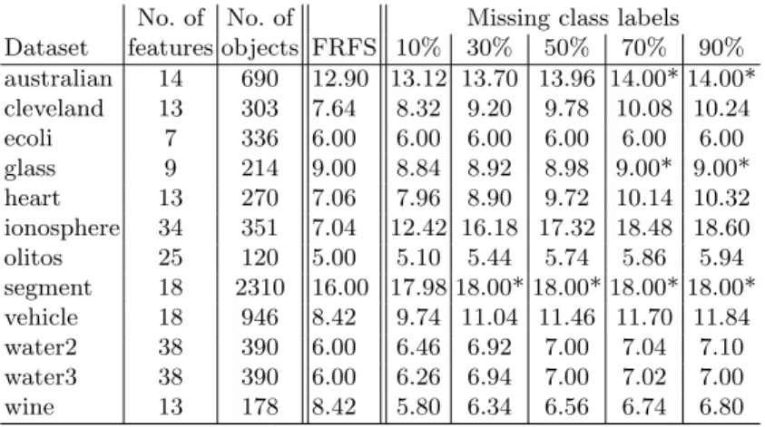
The results of the experimental evaluation are shown in Tables 1-3. The results in Table 1 show that the approach achieves a reduction in the subset sizes for
almost all cases, with a few small notable exceptions of theaustralian andglass datasets when the number of missing labels is greater than 70%. The segment dataset also shows a similar pattern starting at 30%. It should be noted however that the corresponding level of reduction using FRFS with no missing labels is very small - only a single feature, so this is expected to some degree.
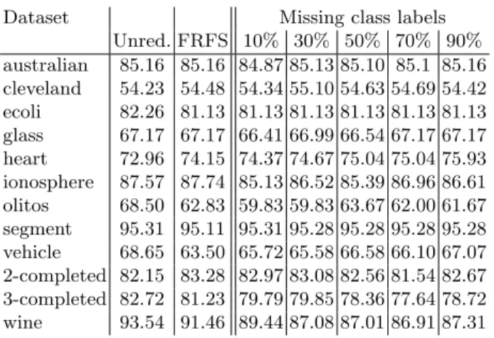
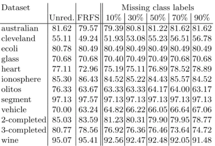
Tables 2 and 3 detail the classification results for the JRip and IBk classi-fier learners respectively. Examining these results, it is clear that even for those cases with high levels of label removal, ssFRFS can still return comparable clas-sification accuracies to the case where no labels have been removed. Clearly, it would be unrealistic to expect that this approach would be able to maintain the robustness of the fully supervised data (no missing labels). After all, there is much discriminative information encoded in class labels, but overall ssFRFS performs well. There is a small decrease in performance when compared to the unreduced data, but the statistical analysis in Tables 4 and 5 shows that no significant differences are observed when the results are compared with the fully supervised approach, regardless of the level of missing labels.
No. of No. of Missing class labels Dataset features objects FRFS 10% 30% 50% 70% 90% australian 14 690 12.90 13.12 13.70 13.96 14.00* 14.00* cleveland 13 303 7.64 8.32 9.20 9.78 10.08 10.24 ecoli 7 336 6.00 6.00 6.00 6.00 6.00 6.00 glass 9 214 9.00 8.84 8.92 8.98 9.00* 9.00* heart 13 270 7.06 7.96 8.90 9.72 10.14 10.32 ionosphere 34 351 7.04 12.42 16.18 17.32 18.48 18.60 olitos 25 120 5.00 5.10 5.44 5.74 5.86 5.94 segment 18 2310 16.00 17.98 18.00* 18.00* 18.00* 18.00* vehicle 18 946 8.42 9.74 11.04 11.46 11.70 11.84 water2 38 390 6.00 6.46 6.92 7.00 7.04 7.10 water3 38 390 6.00 6.26 6.94 7.00 7.02 7.00 wine 13 178 8.42 5.80 6.34 6.56 6.74 6.80
* denotes that no reduction took place
Table 1: Average subset size in terms of original number of features.
5
Conclusion
This paper has presented a new approach to feature selection for semi-supervised data. One of the primary motivations behind the development of the approach was to propose a means of carrying out FS when some of the data class labels are missing. Indeed, there is no bound on the number of labelled data objects required and even if all labels are missing, the approach will still return a valid fuzzy-rough (super)reduct. This appealing property means that no consideration
Dataset Missing class labels Unred. FRFS 10% 30% 50% 70% 90% australian 85.16 85.16 84.87 85.13 85.10 85.1 85.16 cleveland 54.23 54.48 54.34 55.10 54.63 54.69 54.42 ecoli 82.26 81.13 81.13 81.13 81.13 81.13 81.13 glass 67.17 67.17 66.41 66.99 66.54 67.17 67.17 heart 72.96 74.15 74.37 74.67 75.04 75.04 75.93 ionosphere 87.57 87.74 85.13 86.52 85.39 86.96 86.61 olitos 68.50 62.83 59.83 59.83 63.67 62.00 61.67 segment 95.31 95.11 95.31 95.28 95.28 95.28 95.28 vehicle 68.65 63.50 65.72 65.58 66.58 66.10 67.07 2-completed 82.15 83.28 82.97 83.08 82.56 81.54 82.67 3-completed 82.72 81.23 79.79 79.85 78.36 77.64 78.72 wine 93.54 91.46 89.44 87.08 87.01 86.91 87.31
Table 2: Classification accuracy using JRip
needs to be given to any tunable parameters in order to account for differing levels of supervision of the data. Indeed the experimental evaluation has demon-strated that the approach is particularly useful even with high levels of missing labels.
The ideas described in this paper offer some new directions for further de-velopment. In particular, other supervised fuzzy-rough approaches could be ex-tended in a similar way to that proposed in this paper, including the fuzzy discernibility matrix-based approaches described in [5]. Also, the idea of object weighting could be incorporated [9], where objects with missing labels are con-sidered to be less important in the calculations when compared to those that are labelled.
The basic semi-supervised concepts could be further generalised to the situa-tion where both condisitua-tional and decision features may be missing from the data. This could form the basis for a number of approaches for performing feature selection on sparse data. For the work described here, the fuzzy connectives and similarities are the same as those used for the typical supervised approaches, but it would be interesting to investigate the influence of different choices in this regard.
Acknowledgment
Neil Mac Parthal´ain would like to acknowledge the financial support for this research through NISCHR (National Institute for Social Care and Health Re-search)Wales, Grant reference: RFS-12-37. Sarah Vluymans is supported by the Special Research Fund (BOF) of Ghent University. Chris Cornelis was partially supported by the Spanish Ministry of Science and Technology under the project TIN2011-28488 and the Andalusian Research Plans P11-TIC-7765, P10-TIC-6858 and P12-TIC-2958.
Dataset Missing class labels Unred. FRFS 10% 30% 50% 70% 90% australian 81.62 79.57 79.39 80.81 81.22 81.62 81.62 cleveland 55.11 49.24 51.93 53.08 55.23 56.51 56.78 ecoli 80.78 80.49 80.49 80.49 80.49 80.49 80.49 glass 70.68 70.68 70.40 70.49 70.49 70.68 70.68 heart 77.11 72.96 75.19 75.11 76.89 78.52 78.89 ionosphere 85.30 86.43 84.52 85.22 84.43 85.57 84.52 olitos 76.33 63.67 63.33 63.33 64.17 64.00 63.17 segment 97.13 97.57 97.13 97.13 97.13 97.13 97.13 vehicle 70.00 63.24 64.82 66.22 66.05 66.64 67.06 2-completed 85.03 83.59 81.23 80.31 79.90 79.95 78.77 3-completed 80.77 78.56 76.92 76.36 76.46 73.64 74.72 wine 95.07 95.41 92.56 92.47 92.48 92.05 91.48
Table 3: Classification accuracy using IBk
FRFS+IBk (0%) R+ R− P-value ssFRFS+IBk (10%) 43.0 23.0 ≥0.2 ssFRFS+IBk (30%) 35.0 31.0 ≥0.2 ssFRFS+IBk (50%) 31.0 35.0 ≥0.2 ssFRFS+IBk (70%) 36.5 41.5 ≥0.2 ssFRFS+IBk (90%) 40.5 37.5 ≥0.2
Table 4: Comparison of FRFS with ssFRFS for IBk
References
1. W.W. Cohen. Fast effective rule induction, Proceedings of the 12th International Conference on Machine Learning, pp. 115–123, 1995.
2. C. Cornelis, R. Jensen, G. Hurtado Mart´ın, D. ´Sl¸ezak. Attribute Selection with Fuzzy Decision Reducts, Information Sciences, vol. 180, no. 2, pp. 209–224, 2010. 3. D. Dubois and H. Prade. Putting Rough Sets and Fuzzy Sets Together,inIntelligent
Decision Support, pp. 203–232, 1992.
4. A. Frank and A. Asuncion. UCI Machine Learning Repository [http://archive.ics.uci.edu/ml]. Irvine, CA: University of California, School of Information and Computer Science, 2010.
5. R. Jensen and Q. Shen. New Approaches to Fuzzy-Rough Feature Selection, IEEE Transactions on Fuzzy Systems, vol. 17, no. 4, pp. 824–838, 2009.
6. R. Jensen, A. Tuson, and Q. Shen. Finding rough and fuzzy-rough set reducts with SAT, Information Sciences, vol. 255, pp. 100–120, 2014.
7. Z. Pawlak. Rough Sets: Theoretical Aspects of Reasoning About Data, Kluwer Aca-demic Publishing, 1991.
8. A.M. Radzikowska and E.E. Kerre. A comparative study of fuzzy rough sets, Fuzzy Sets and Systems, vol. 126, no. 2, pp. 137–155, 2002.
9. S. Widz and D. ´Sl¸ezak. Attribute subset quality functions over a universe of weighted objects. Proceedings of RSEISP 2014, pp. 99-110, 2014.
FRFS+JRip (0%) R+ R− P-value ssFRFS+JRip (10%) 52.0 14.0 0.10156 ssFRFS+JRip (30%) 44.0 22.0 ≥0.2 ssFRFS+JRip (50%) 38.0 28.0 ≥0.2 ssFRFS+JRip (70%) 41.5 24.5 ≥0.2 ssFRFS+JRip (90%) 42.5 23.5 ≥0.2
Table 5: Comparison of FRFS with ssFRFS for JRip
10. F. Wilcoxon. Individual comparisons by ranking methods, Biometrics bulletin, vol. 1, no. 6, pp. 80–83, 1945.