Modeling and Forecasting Naira / USD Exchange Rate In Nigeria: a Box - Jenkins ARIMA approach

(1)

MPRA

Munich Personal RePEc Archive

Modeling and Forecasting Naira / USD

Exchange Rate In Nigeria: a Box

-Jenkins ARIMA approach

Thabani Nyoni

University of Zimbabwe

22 August 2018

Online at

https://mpra.ub.uni-muenchen.de/88622/

MPRA Paper No. 88622, posted 26 August 2018 07:06 UTC

(2)

Modeling and Forecasting Naira / USD Exchange Rate In Nigeria: a Box – Jenkins ARIMA approach

Thabani Nyoni

Department of Economics, University of Zimbabwe, Harare, Zimbabwe

Email: nyonithabani35@gmail.com

Abstract

In the financial as well as managerial decision making process, forecasting is a crucial element (Majhi et al, 2009). Most research have been made on forecasting of financial and economic variables through the help of researchers in the last decades using series of fundamental and technical approaches yielding different results (Musa et al, 2014). The theory of forecasting exchange rate has been in existence for many centuries where different models yield different forecasting results either in the sample or out of sample (Onasanya & Adeniji, 2013). A country’s exchange rate is one of the most closely monitored indicators, as fluctuations in exchange rates can have far reaching economic consequences (Ribeiro, 2016). The recent financial turmoil all over the world demonstrates the urgency of perfect information of the exchange rates (Shim, 2000). Understanding the forecasting of exchange rate behaviour is important to monetary policy (Simwaka, 2007). One of the important variables that have considerable influence on other socio – economic variables in Nigeria is the Nigerian naira / dollar exchange rate (Ismail, 2009). Owing to the critical role played by exchange rate dynamics in international trade and overall economic performance of all countries in general, the need for a good forecasting tool cannot be ruled out. In this study, we model and forecast the Naira / USD

exchange rates over the period 1960 – 2017. Our diagnostic tests such as the ADF test indicate

that EXC time series data is I (1). Based on the minimum AIC value, the study presents the ARIMA (1, 1, 1) model as the optimal model. The ADF test further indicates that the residuals of the ARIMA (1, 1, 1) model are stationary and thus bear the characteristics of a white noise process. It is also important to note that our forecast evaluation statistics, namely ME, RMSE,

MAE, MPE, MAPE and Theil’s U absolutely show that our forecast accuracy is quite good. Our

forecast actually indicates that the Naira will continue to depreciate. The main policy implication from this study is that the Central Bank of Nigeria (CBN), should devalue the Naira in order to not only restore exchange rate stability but also encourage local manufacturing and promote foreign capital inflows.

Key Words: ARIMA, Exchange rate, Forecasting, Nigeria

JEL Codes: C53, E37, E47, F31, F37, O24

I. Introduction & Background

Foreign exchange is a major issue in the discussion of world economy (Etuk et al, 2016).

(3)

Exchange rate modeling and forecasting is important for policy making (Hina & Qayyum, 2015). Forecasting exchange rate is crucial as it has significant impact on the macroeconomic fundamentals such as oil price, interest rate, wage, unemployment and the level of economic

growth (Ramzan et al, 2012). Foreign exchange markets are among the most important and the

largest financial markets in the world with trading taking place twenty – four hours a day around the globe and trillions of dollars of different currencies transacted each day (Khashei & Bijari, 2011).

The exchange rate1 is a relative price that measures the worth of a domestic currency in terms of another currency (Nwankwo, 2014). Exchange rate is seen as the relative value of the domestic currency in terms of foreign exchange (Mussa, 1984; Ahmed, 2001). Exchange rate is the currency rate of one country expressed in terms of the currency of another country (Khan & Jain, 2009). The foreign exchange rate is the price of one currency in terms of another currency (Samuelson & Nordhaus, 1998; Usman & Adejare, 2013; CBN, 2016). Foreign exchange connotes the process of trading domestic currencies for foreign ones at varying exchange rates (Oleka et al, 2014). Exchange rate is the rate at which two national currencies exchange for each other (Lipsey & Crystal, 1995). Exchange rate is often expressed as the amount of domestic currency needed to buy one unit of foreign currency (Dornbusch et al, 2005).

The exchange rate serves as an important price factor in the economy (Klein & Shambaugh, 2012). It is a measurement of the price of country’s domestic currency relative to a foreign basket of goods or prices (Gourinchas, 1999). It determines the relative prices of domestic and foreign goods, as well as the strength of external sector participation in the international trade (Mohammed & Abdulmuahymin, 2016). In fact, foreign exchange is the component that is widely used on daily basis for settlement of international transactions and international bills

(Oleka et al, 2014). The exchange rate of a Naira per US dollar is the amount of Naira required

to obtain one unit of US dollar (Jhingan, 2005; Campbell, 2010; Omojolaibi & Gibadebo, 2014). For a country like Nigeria, the price of foreign exchange plays a highly significant role in the ability of the economy to attain optimal productive capacity (Ogiogio, 1996).

Foreign exchange rates are among the most important prices in international monetary markets (Rahim et al, 2018). They affect the economic activity, foreign trade and the distribution of wealth among countries (Tan, 2009). The stability of the exchange rate is today a formidable bedrock of all economic activities (Taiwo & Adesola, 2013). The centrality of exchange rates in the formulation of monetary policy derives from the fact that for most countries, the prevailing objective of monetary policy is price stability (Adeoye & Saibu, 2014). Therefore, central banks should pay special attention to exchange rates and the value of their domestic currency (Dilmaghani & Tehranchian, 2015). The main objectives of exchange rate policy in Nigeria are to preserve the value of the Naira and to maintain enough foreign exchange reserves (Oleka & Okolie, 2016). In Nigeria, the central bank maintains the stability of the Naira exchange rate in order to achieve its objective of maintaining price stability because domestic prices (inflation and interest rates) are very responsive to exchange rate fluctuations (CBN, 2016).

1 _{Various definitions of the term “exchange rate” exist. It is clear that there is no apparent consensus on the} definition of the term “exchange rate”.

(4)

In the modern world, exchange rates of the most successful countries tend to be floating (Sullivan, 2001). Forecasting of the exchange rate is the foremost endeavor of the practitioners and researchers in the spree of international finance, particularly in the case of the exchange rate

which is floating (Hu et al, 1999). Economic growth is one of the fundamental macroeconomic

policy objectives which countries all over the world continue to strive to achieve and Nigeria is not an exception (Nyoni & Bonga, 2018). The Nigerian economy ambitiously aspires to become

one of the twenty largest economies in the world by 2020 and the 12th largest economy by 2050

(CBN, 2009). One of the surest way to achieve the afore – stated goal is to pursue vigorously rapid and sustainable economic growth and development via well managed exchange rate policy (Obi et al, 2016). Sustainable economic growth mainly depends on a nation’s ability to invest and make efficient and productive use of the resources at its disposal (Nyoni & Bonga, 2017f). The status of a country’s economic well being is reflected by the real exchange rate (Arize & Osang, 2000). Poorly managed exchange rates can be disastrous for economic growth (Rodrick, 2008).

When the domestic income of a country increases, then the country’s currency is likely to depreciate. However, an increase in foreign income would likely lead to appreciation of the currency. Also when a nation has a crave for domestic goods and services, it will likely to appreciation of the currency, while a crave for foreign goods and services will likely lead to depreciation of its currency (Arize & Osang, 2000). If the domestic inflation rate exceeds the global average rate, it will likely lead to its currency’s depreciation. However, if the domestic inflation rate is less than the global average then the chances are that its currency will appreciate (Giovanni, 1988; Islam & Sardar, 2007).

Fluctuations in a nation’s currency or exchange rate exert changes in domestic production costs

(Ngandu, 2008) and also affect the labor market based on channels of appreciation and depreciation of currencies (Nucci & Pozzolo, 2010). A depreciation in the exchange rate increases or promotes the growth of local jobs in the manufacturing and non – manufacturing sectors (Yokoyama et al, 2015). Volatile exchange rates may also increase unemployment through lowering investment in physical capital (Belke & Gros, 2001). Investment may be reduced because higher volatility usually entails increased uncertainty (Nyahokwe & Ncwadi, 2013). Therefore, maintaining exchange rate stability implies controlling a country’s level of

unemployment (Chimnani et al, 2012) and promoting investment. When the monetary authority

allows the exchange rate to be fixed, other macroeconomic variables are volatile. However, when exchange rate is allowed to float, it is known that the exchange rate becomes highly volatile in comparison with other macroeconomic variables (Baxter & Stockman, 1989; Flood & Rose, 1999; MacDonald, 2008).

Many authors, for example; Domac & Shabsign (1999), Takaendesa (2006), Miles (2006), Sibanda et al (2013), Korkmaz (2013), Ahmad et al (2013), Uddin et al (2014) and Chipeta et al

(2017) agree on the important role played by exchange rates on economic growth. In Nigeria,

specifically; authors such as Odusola & Akinlo (2001), Usman (2007), Bakare (2011), Azeez et

al (2012), Akpan & Atan (2012), Obansa et al (2013), Rasaq (2013), Fapetu & Oloyede (2014), Eze & Okpala (2014), Anigbogu et al (2014), Oleka et al (2014), Adelowokan et al (2015), Ali

et al (2015), Obi et al (2016), Isola et al (2016) and Okonkwo et al (2017) confirm that indeed there is need for proper exchange rate management if economic growth is to be sustained. To move Nigeria on a sustainable economic growth trajectory, policy makers should focus on those

(5)

factors that determine economic growth in Nigeria (Nyoni & Bonga, 2018) and foreign exchange rate is one of those factors.

The evolution of the Nigerian foreign exchange market was influenced by such factors as the changing patterns of international trade, institutional changes in the economy and structural shifts in production (CBN, 2011). The oil boom experienced in nineteen seventies led to enhanced foreign exchange receipts; hence the need to develop a local foreign exchange market

became paramount (Mojekwu et al, 2011). Nigeria, like many other low income open

economies, has adopted two main exchange regimes. Direct administrative control exchange rate was used until 1986, when the country changed over to market regulated regime. Nigeria has, and is still experimenting with various market arrangements. As an integral part of Structural Adjustment Programme introduced in 1986, Nigeria adopted the flexible exchange rate through second tier foreign exchange market (Umar & Soliu, 2009). Since then, several variants (Auction System, Dutch Auction System, Wholesale Dutch Auction System and Rental Dutch Auction

System) have been operated in determining the exchange rate of naira to US dollar (Mojekwu et

al, 2011).

Over two decades ago, the Central Bank of Nigeria (CBN) have been intervening in the foreign exchange market (FEM) to support and stabilize the value of the Naira, although the supportive efforts remain temporarily and short – lived (Sanusi, 2004; Adebiyi, 2007). For instance, Nigeria had been one of the most active countries in the FEM between 1993 and 1995 (Adebiyi, 2007; Omojalaibi & Gibadebo, 2014). In the month of December 2014 alone, the CBN spent about $2.3 billion to defend the Naira from losing its value (Nweze, 2015). Also, in another effort to strengthen and stabilize the value of the Naira, the CBN conducted another intervention operation in the first quarter of 2015. The process worth the CBN $4.7 billion (Komolafe, 2015). The main objectives of the central bank interventions in the FEM, especially in countries with floating exchange rates are to prevent exchange rate misalignment, counter disorderly FEM, manage foreign reserve and “lean against the wind” (Basu & Varoudakis, 2013). In most emerging market – oriented economies like Nigeria, preserving a realistic value for the domestic currency is of paramount importance considering the structure of the economy and the desire to balance domestic production and consumption, create and improve the success of foreign exchange earnings and attracts foreign capitals from multi – national corporations (Dayyabu et al, 2016).

Timely forecasting of the exchange rates is able to give important information to the decision makers as well as partakers in the area of the internal finance, buy and sell, and policy making (Alam, 2012). For the giant multinational business units, an accurate forecasting of the exchange rate is crucial since it improves their overall profitability (Huang et al, 2004). The importance of forecasting the exchange rates in practical aspect is that an accurate forecast can render valuable information to the investors, firms and central banks for use in allocation of assets, in hedging risk and in policy formulation (Tindaon, 2015). The significance of exchange rates forecasting stems from the reality that the findings of a given financial decision made today is conditional on the exchange rate which will be prevailed in the upcoming period. For this reason forecasting exchange rate is essential for various international financial transactions, namely speculation, hedging as well as capital budgeting (Moosa, 2008). In this study, I rely on the Box – Jenkins ARIMA approach to model and forecast the Naira / USD exchange rate in Nigeria over the period 1960 – 2017. The rest of the paper is structured in chronological order as follows:

(6)

literature review, materials & methods, diagnostic tests & model evaluation, results: presentation, interpretation & discussion and conclusion & policy implications.

II. Literature Review

Theoretical Literature Review

While there are a number of theories of exchange rate determination, in this study we will briefly discuss only five most popular ones and these are namely: the Mint Parity Theory, the Quantity Theory of Money, the Tightening Monetary Policy Theory, the Purchasing Power Parity Theory and the Balance of Payment Theory.

The Mint Parity Theory (MPT)

The MPT is associated with the working of the international gold standard (Brown, 2008). Under

this system, considering the period 1955 – 1970, when the exchange rates were pegged into gold

under the Bretton Woods System, the currency in use was made of gold or was convertible into gold at a fixed rate. In this case, the value of the currency unit was defined in terms of certain weight of gold and the central bank of the country concerned was always ready to buy and sell gold at the specified price. The rate at which such currency could be converted into gold is called the mint price of gold (Oleka et al, 2014).

The Quantity Theory of Money (QTM)

Hinged on the monetarist school of thought, the QTM is one of the simplest models for determining long run equilibrium exchange rate. In their diagnosis of the QTM, as noted by Nyoni (2018k); monetarists finalize that any change in the quantity of money affects only the price level, leaving the real sector of the economy totally unaffected. In the context of international economics, or simply the so – called international version of the QTM, the increase in money supply also manifests through a proportionate increase in the exchange rate. As noted

by Oleka et al (2014), the exchange rate can be viewed as determined by the demand for money,

which is in turn influenced positively by the rate of growth of the real economy and negatively by the inflation rate. Therefore, we cannot rule out the fact that the growth of the real economy

impacts significantly on a nation’s currency position. According to Ude (1999), a defect of the

international QTM is that it cannot account for fluctuations in the real exchange rate as opposed to simply the nominal exchange rate.

The Tightening Monetary Policy Theory (TMPT)

The TMPT argues that an increase in the real interest rate due to a tightening monetary policy causes the currency to appreciate more in the short run than it will in the long run. Given that the rate of return on domestic assets may be higher because of the monetary tightening; international investors may be willing to hold foreign assets, especially if they anticipate the value of the domestic currency to fall in the future. Oleka et al (2014) argues that an advantage of the TMPT over the international QTM is that it can account for fluctuations in the real exchange rate.

(7)

This is an economic theory used in determining the relative value of currencies, estimating the amount of adjustment needed in the exchange rate between countries, in order for the exchange

rate to be equivalent to each currency’s purchasing power (CBN, 2011). This theory recognizes

inflation levels and trends as important determinants of exchange rate of a currency both in emerging and developed economies (Scott, 2008). PPPT avers that a currency will lose value if there is a high level of inflation in the country or if inflation levels are perceived to be going up. This is attributed to the fact that inflation erodes the purchasing power, thus demand for that

specific currency. According to Oleka et al (2014), a currency may sometimes strengthen when

inflation rises due to expectations that the central bank of the country concerned will raise short – term interest rates to combat rising inflation. PPPT, as noted by Obadan (2006); concludes that the equilibrium exchange rate between two invertible paper currencies is determined by the equality of their purchasing power (that is, their relative prices).

Balance of Payment Theory (BOPT)

This theory stipulates that under free exchange rates, the exchange rate of the currency of a

country depends upon its balance of payment position (Oleka et al, 2004). A favourable balance

of payment raises the exchange rate, while an unfavorable balance of payments reduces the exchange rate (Jhingan, 2004). Thus the theory implies that the exchange rate is determined by the equilibrium in the balance of payment (Oleka et al, 2014).

Empirical Literature Review

The table below shows a summary of the reviewed empirical studies done in Nigeria and elsewhere:

Table 1

Author Year Country Study Period Method Key Findings

Mojekwu et al 2011 Nigeria 1974 – 2008 AR (1); ARIMA (1, 1, 1); MA (1); IMA (1, 1); SARIMA (0, 0, 0)(1, 1, 1)12; Simple,

Double, Linear, Damped – trend Linear and Seasonal Exponential Smoothing; Winters Method.

Central Bank of Nigeria exchange is the most stable while Bureau de change and inter – bank exchange rates to US dollar fluctuate over the period under investigation.

Etuk 2012 Nigeria January 2004 –

December 2011

SARIMA models SARIMA (0, 1, 1)x(1, 1, 1)12

model was found adequate.

Etuk 2013 Nigeria January 2004 –

December 2011

SARIMA models The (0, 1, 1)x(1, 1, 1)12 SARIMA

is the best fit model. Osarumwense &

Waziri

2013 Nigeria January 1990 – December 2010

ARIMA models ARIMA (0, 1, 1) is appropriate. Onasanya &

Adeniji

2013 Nigeria January 1994 – December 2011

ARIMA models The best fit model is ARIMA (1, 2, 1) model.

Nwankwo 2014 Nigeria 1982 – 2011 ARIMA models The best fit model is ARIMA (1,

1, 0).

Etuk 2014 Nigeria 8 December 2012 –

30 March 2013

model is the best fit model. Musa et al 2014 Nigeria June 2000 – July

2011

GARCH models GJR – GARCH & TGARCH models show the existence of statistically significant asymmetry effect.

(8)

Mbaga & Olubusoye 2014 Nigeria 18 April 2007 – 3 September 2012 FROEXNN and ARIMA models

FOREXNN models are superior to ARIMA models.

Olatunji & Bello 2015 Nigeria January 2000 – December 2012

ARMA & ARIMA models

ARIMA (1, 1, 2) and ARMA (1, 1) models are optimal. Mohammed &

Abdulmuahymin

2016 Nigeria 1972 – 2014 ARIMA models ARIMA (0, 2, 1) is the best fit model.

Chamalwa et al 2016 Nigeria 1981 – 2012 ARIMA models ARIMA (2, 1, 2) is the best fit model.

Etuk et al 2016 Nigeria 22 September 2015 –

16 March 2016

model is the best fit model. Ajao et al 2017 Nigeria 1972 – 2017 ARIMA models ARIMA (0, 1, 0) is the optimal

model. Khashif et al 2008 Pakistan 1 July 2001 – 30 June

2007

ARIMA, GARCH and State Space models

The State Space model provides the best performance among all the models.

Kadilar et al 2009 Turkey 3 January 2005 – 28 January 2008

ANN, ARIMA and ARCH models

ANN is more accurate than ARIMA and ARCH models

Botha & Pretorius 2009 South Africa 1990 quarter 1 – 2006 quarter 4 Various univariate and multivariate models

The multivariate models outperformed the univariate models (except for random walk model) in the short – run forecasts, one step ahead, while the multivariate models, performed better in the longer – run forecasts.

Fat & Dezsi 2011 Romania 3 January 2011 – 22 April 2011

Exponential smoothing and ARIMA models

Romanian Leu is appreciating against other currencies.

Appiah & Adetunde

2011 Ghana January 1994 –

December 2010

ARIMA models ARIMA (1, 1, 1) model is the most appropriate model. Ramzan et al 2012 Pakistan July 1981 – May

2010

ARMA, ARCH and GARCH models

GARCH (1, 2) is found to be best in removing persistence in volatility while EGARCH (1, 2) successfully overcome the leverage effect in the exchange rate returns under study.

Alam 2012 Bangladesh 3 July 2006 – 30

April 2010

AR and ARMA models

Both the ARMA and AR models jointly outperform other models, in terms of in – sample data set. Nanayakkara et

al

2014 Sri Lanka 1 January 2007 – 18 November 2011

Time series and Neural Network approaches

ANN performs better than GARCH models.

Pedram & Ebrahimi

2014 Iran 1 November 2010 –

30 June 2013

Neural Networks Neural Network is far much better than ARIMA.

Babu & Reddy 2015 India January 2010 – April 2015

ARIMA, Neural Networks and Fuzzy Neurons

In predicting exchange rate market in India, ARIMA model does better than complex non – linear models such as Neural Networks and Fuzzy Neurons.

Chi et al 2015 China 25 July 2005 – 25

March 2014

ARFIMA, SVM and BPNN

The prediction performance of the nonlinear combination model is better than the single models. Etuk & Natamba 2015 Uganda July 1990 –

November 2014

SARIMA models SARIMA (0, 1, 1)x(0, 1, 1, 1)12 is

the optimal model.

Ayekple et al 2015 Ghana January 2004 –

February 2015

ARIMA models The exchange rate of the Ghana Cedi to the American Dollar will increase continuously for the years 2016, 2017 and 2018.

Biswajit 2015 India August 1994 – April

2014

ARIMA, ARCH and GARCH models

The random walk model outperforms ARIMA and ARCH/GARCH models for

(9)

forecasting exchange rates of Indian Rupee under the in – sample and the out – of – sample period.

Ngan 2016 Vietnam January 2013 –

December 2015

ARIMA models ARIMA model is absolutely suitable for forecasting. Mustafa et al 2017 Malaysia 1 November 2010 –

30 August 2016 Hybrid ARIMA – EGARCH models; hybrid ARIMA – GARCH models.

ARIMA – EGARCH model fits the data better and also performs better in terms of capturing volatility clustering and leverage effects in the series.

Varenius 2017 Sweden January 2000 –

December 2015

ARIMA and VAR models

VAR (1) generates the most accurate forecasts during a 1 – month horizon, while the ARIMA (1, 1, 0) is the more suitable model during a 3 – month horizon. Both models outperform a random walk.

III. Materials & Methods

Empirical Modeling & Estimation The Moving Average (MA) Process

Given that t is a purely random process with mean zero and varience σ2and where ℓ is the lag

operator and EXCt is the Naira / USD exchange at time t; a process defined by equation [1]

below is called an MA (z) process.

EXCt= ∑𝑧_𝑖=1𝛽iℓi t+ t……….……….. [1]

Or

(ℓ)=k(ℓ) ……….……… [2]

where:

k(ℓ)=1+ 1ℓ+…+ zℓz………..……….. [3] The Autoregressive (AR) Process

Equation [4] below is known as an AR (r) process.

EXCt= ∑𝑟_𝑖=1ɑiℓiEXCt+ t………...……….. [4] Or ɑ(ℓ)EXCt= t……… [5] where ɑ(ℓ)= (ℓ) ………...……….. [6] where (ℓ)=1-ɑ1ℓ-ɑ2ℓ2…ɑrℓr……….. [7]

(10)

The Autoregressive Moving Average (ARMA2) Process

Box & Jenkins (1976) combined the autoregressive and moving average terms in order to come up with an ARMA model (Nyoni, 2018i). Combining equations [1] and [4], an ARMA (r, z) process is specified as follows:

(ℓ)EXCt=k(ℓ) t………..……… [8]

where (ℓ) and k(ℓ) are polynomials of orders r and z respectively, simply defined as in

equations [3] and [7].

The Autoregressive Integrated Moving Average (ARIMA3) Process

The ARIMA modeling approach proposed by Box & Jenkins (1976) is recognized as a benchmark technique in modeling and forecasting methods because of its structured modeling basis and acceptable forecasting performance (Goh & Teo, 2000). ARIMA models are a set of models that describe the process as a function of its own lags and white noise process (Box & Jenkins, 1974). Making prediction in time series using univariate approach is best done by

employing the ARIMA models (Alnaa & Ahiakpor, 2011). A stochastic process EXCt is called

an ARIMA (r, d, z) process if it is I (d) and the d times differenced process has an ARMA

representation. If the sequence, ∆d

EXCt satisfies an ARMA (r, z) process; what it implies is that

the sequence of EXCt also satisfies the ARMA (r, d, z) process such that:

∆d

EXCt= ∑𝑟_𝑖=1ɑi∆dℓiEXCt+ ∑𝑧_𝑖=1𝛽iℓi t+ t……….……….. [9]

Where ∆ is the difference operator, vector ɑ ϵⱤr_{and ϵ}_Ɽz Model Specification

The ARIMA (1, 1, 1) model, chosen based on table 8; is specified below:

(1-ℓ)EXCt=ɑℓEXCt+(1- 1ℓ) t+ t……….. [10]

The Box – Jenkins Methodology

2

The ARMA (r, z) can only be used for stationary time series data. However, in reality, many time series are non – stationary since they usually contain trends and or seasonal patterns. This implies that, from an application point of view; ARMA models are not appropriate for describing non – stationary time series (Nyoni, 2018i). The family of univariate time series models is not complete without a third element, orders of integration (Wang, 2009).

3

One of the most popular and frequently used stochastic time series is the Autoregressive Integrated Moving Average (ARIMA) model (Box & Jenkins, 1970; Hipel & McLeod, 1994; Cochrane, 1997; Zhang, 2003). The popularity of the ARIMA model is mainly due to its flexibility to represent several varieties of time series with simplicity as well as the associated Box – Jenkins methodology (Box & Jenkins, 1970; Hipel & McLeod, 1994; Zhang, 2003; Hamzacebi, 2008). The main advantage of ARIMA forecasting is that it requires data on the time series in question only. First, this feature is advantageous if one is forecasting a large number of time series. Second, this avoids a problem that occurs sometimes with multivariate models. Third, with multivariate models, timeliness of data can be a problem (Meyler et al, 1998). ARIMA models frequently outperform more sophisticated structural models in terms of short – run forecasting ability (Litterman, 1986; Stockton & Glassman, 1987). However, ARIMA models are essentially backward looking. As such, they are generally poor at predicting turning points, unless the turning point represents a return to a long – run equilibrium (Meyler et al, 1998).

(11)

The Box – Jenkins methodology is shown below: Figure 1

NO

YES

The first step towards model selection is to difference the series in order to achieve stationarity. Once this process is over, the researcher will then examine the correlogram in order to decide on the appropriate orders of the AR and MA components. It is important to highlight the fact that

this procedure (of choosing4 the AR and MA components) is biased towards the use of personal

judgement because there are no clear – cut rules on how to decide on the appropriate AR and MA components. Therefore, experience plays a pivotal role in this regard. The next step is the estimation of the tentative model, after which diagnostic checking shall follow. Diagnostic checking is usually done by generating the set of residuals and testing whether they satisfy the characteristics of a white noise process. If not, then there would be need for model re – specification and repetition of the same process; this time from the second stage. The process may go on and on until an appropriate model is identified (Nyoni, 2018i).

4

In this study, we employ the Akaike Information Criterion (AIC). Diagnostic checking

Difference the series to achieve stationarity

Parameter estimation Tentative model

identification

Use the model to generate forecasts

(12)

Data Collection

An extensive time series data is required for univariate time series forecasting (Wabomba et al, 2016). More than 50 observations are recommended in order to build a reliable ARIMA model (Chatfield, 1996; Meyler et al, 1998). In line with Chatfield (1996), Meyler et al (1998) and

Wabomba et al (2016) amongst others; this study is based on 57 observations of annual Naira /

USD5 exchange rates (EXC). All the data used in this study was collected from the World Bank.

IV. Diagnostic Tests & Model Evaluation

Stationarity (Unit Root) Tests Graphical Test

Stationarity of a series can be tested graphically, as already shown by Gujarati (2004). Figure 2

The time plot above indicates that the time series data is not stationary simply because it shows an upward trend which implies that the mean of EXC is changing over time and thus there is no stability in the variance of the time series data.

The Correlogram

The correlogram below, presented in graphical form; confirms the non – stationarity of the EXC

time series data. The most striking feature of this correlogram is that the autocorrelation coefficients are quite high at various lags and this is typical for non – stationary time series data.

5

United States Dollars

0 50 100 150 200 250 300 1960 1970 1980 1990 2000 2010

(13)

Figure 3

ADF Test

The Augmented Dickey Fuller (ADF test) was used to check the stationarity of the EXC series. The general ADF test is done by running the following regression equation:

EXCt= ct EXCt-1+∑𝑝−1_𝑖=1∆EXCt-i+ t………...……….. [11]

Where ct is a deterministic function of the time index t and ∆EXCj=EXCj-EXCj-1 is the

differenced series of EXCt. The null hypothesis H0: =1 is tested against the alternative

hypothesis Ha: ≤1 using equation [11] above. If the null hypothesis is rejected, then the time

series is stationary. The results of the ADF tests done in this study are shown below: Levels: intercept

Table 2

Variable ADF Statistic Critical Values Conclusion

EXC 2.531066 -3.550396 @1% Not stationary

-2.913549 @5% Not stationary

-2.594521 @10% Not stationary

Levels: trend & intercept Table 3

EXC 0.089628 -4.127338 @1% Not stationary

-3.490662 @5% Not stationary -1 -0.5 0 0.5 1 0 2 4 6 8 10 12 lag ACF for EXC

+- 1.96/T^0.5 -1 -0.5 0 0.5 1 0 2 4 6 8 10 12 lag PACF for EXC

(14)

-3.173943 @10% Not stationary Levels: without intercept and trend & intercept

Table 4

EXC 3.656847 -2.606163 @1% Stationary

-1.946654 @5% Stationary

Tables 2 and 3 indicate that the EXC series is basically not stationary at levels. Although table 46 indicates that the series is stationary without intercept and trend & intercept, we need to proceed to check for stationarity at first differences as shown in tables 5 – 7 below.

The Correlogram (at First Differences)

For a purely white noise process, the autocorrelations at various lags hover around zero (Gujarati, 2004). The autocorrelations below, especially those between lags 2 nd 12; generally hover around zero, pointing to the conclusion that D (EXC) is stationary. We also note that in the correlogram below, there are no spikes outside the bands; hence confirming that the series is now stationary. Figure 4 1st difference: intercept Table 5 6

We do not base our analysis much on table 4 since the EXC series exhibits a trend (up – wards sloping).

-0.3 -0.2 -0.1 0 0.1 0.2 0.3 0 2 4 6 8 10 12 lag ACF for d_EXC

+- 1.96/T^0.5 -0.3 -0.2 -0.1 0 0.1 0.2 0.3 0 2 4 6 8 10 12 lag PACF for d_EXC

(15)

D(EXC) -5.713333 -3.552666 @1% Stationary

1st difference: trend & intercept Table 6

D(EXC) -6.422545 -4.130526 @1% Stationary

1st difference: without intercept and trend & intercept Table 7

D(EXC) -5.253249 -2.606911 @1% Stationary

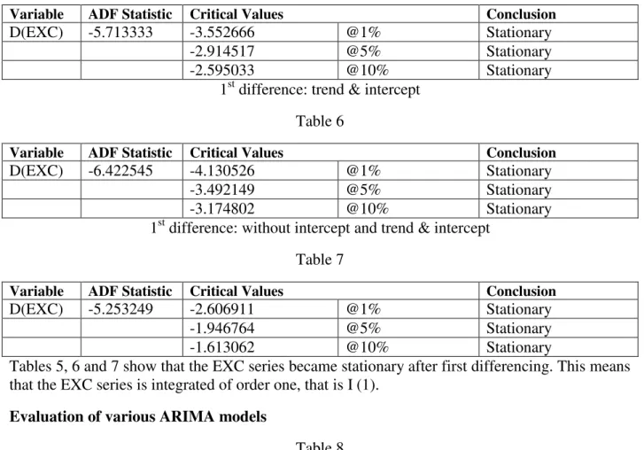
Tables 5, 6 and 7 show that the EXC series became stationary after first differencing. This means that the EXC series is integrated of order one, that is I (1).

Evaluation of various ARIMA models

Table 8 Model AIC ARIMA (1, 1, 1) 462.8502 ARIMA (1, 1, 2) 463.2574 ARIMA (2, 1, 1) 463.3339 ARIMA (1, 1, 3) 465.2568 ARIMA (3, 1, 1) 465.2276

Table 8 above shows that the ARIMA (1, 1, 1) model has the lowest AIC value and is therefore chosen as the optimal model.

ADF test of the Residuals from the ARIMA (1, 1, 1) model

Levels: intercept Table 9

t -6.849788 -3.555023 @1% Stationary

Levels: trend & intercept Table 10

(16)

t -6.793772 -4.133838 @1% Stationary

Levels: without intercept and trend & intercept Table 11

t -6.766794 -2.607686 @1% Stationary

Tables 9, 10 and 11 show that the residuals of the ARIMA (1, 1, 1) model satisfy the characteristics of a white noise process. Therefore, the ARIMA (1, 1, 1) model is adequate and can be used for forecasting and control.

V. Results: Presentation, Interpretation & Discussion

Descriptive Statistics Table 12 Description Statistic Mean 52.275 Median 5.95 Minimum 0.55 Maximum 265 Standard deviation 72.958 Skewness 1.1791 Excess Kurtosis 0.27064

As shown in the table above, the mean is positive. The difference between the minimum and maximum is 264.45 and is quite large. However, it does not indicate the existence of outliers but that the EXC series in ever increasing, thus a depreciating exchange rate ever since. The skewness coefficient is positive as shown, implying that our series has a long right tail and is non

– symmetric. Nyoni & Bonga (2017h) reiterate that the rule of thumb for kurtosis is that it should be around 3 for normally distributed variables and yet in this study kurtosis has been found to be 0.27064 indicating that the EXC series is not normally distributed.

ARIMA (1, 1, 1) model results

Table 13

Variable Coefficient Standard Error z p – value

AR (1) 0.978826 0.108807 8.996 0.0000

(17)

The model can also be represented as follows:

D(EXCt)=0.978826D(EXCt-1) –0.893065 t-1 ………..………. [12]

p – value (0.0000) (0.0000) Std. Error (0.108807) (0.180878)

Results Interpretation

Both coefficients of the AR (1) and MA (1) components are statistically significant at 1% level of significance. The coefficient of the AR (1) component is positive while the coefficient of the MA (1) component is negative as conventionally expected. The AR (1) coefficient is 0.978826 and is thus close to one, implying that the series returns to its mean slowly. The MA (1) coefficient is -0.872319 and represents the fraction of last period’s shock7 that is still felt in the current period. While these results are not similar to any previous study done in Nigeria, they are indeed consistent with the findings of Appiah & Adetunde (2011) who found that an ARIMA (1, 1, 1) model was the optimal exchange rate forecasting model for Ghana.

Forecast graph

Figure 5

7

In the context of Nigeria, such shocks could be things like unpredictable political events (e.g unconstitutional removal of a political administration), droughts, Boko Haram insurgence etc.

0 50 100 150 200 250 300 350 400 1980 1990 2000 2010 2020 95 percent interval EXC forecast

(18)

The graph above indicates that Naira / USD exchange rate is likely to progress at an increasing rate. The implication is that the Naira is likely to continue depreciating against the USD as shown below in figure 6.

Predicted Annual Naira / USD exchanges over the period 2018 – 2022

Figure 6

Confidence Ellipse

Figure 7

The graph above indicates the region in which the realization of the two test statistics must lie for us not to reject the null hypothesis. The graph apparently confirms the accuracy of our forecast.

277.07 288.89 300.46 311.79 322.87 270 280 290 300 310 320 330 2017 2018 2019 2020 2021 2022 2023 Na ira /US D e x cha ng e ra tes Year

EXC Linear (EXC)

-1.4 -1.3 -1.2 -1.1 -1 -0.9 -0.8 -0.7 -0.6 -0.5 -0.4 0.7 0.8 0.9 1 1.1 1.2 1.3 0.979, -0.872 phi_1

(19)

Forecast Evaluation Statistics

Table 14

Forecast Evaluation Statistic Statistic

Mean Error (ME) 2.428

Root Mean Squared Error (RMSE) 13.222

Mean Absolute Error (MAE) 4.6945

Mean Percentage Error (MPE) 5.1282

Mean Absolute Percentage Error (MAPE) 8.6497

Theil’s U 0.97215

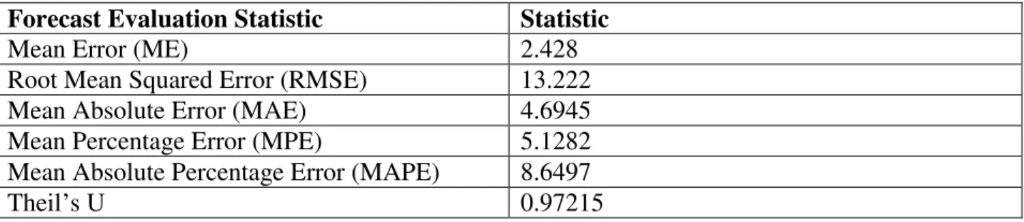
The ME is a measure of the average deviation of forecasted values from actual ones. Since it shows the direction of the error, it is usually termed as the Forecast Bias. A desirable ME must be closer to zero. Our ME is 2.428 which is not far away from zero, indicating that our forecast is indeed good. The RMSE is nothing but the square root of the calculated MSE and must be as small as possible; our RMSE is 13.222 and is generally acceptable. The MAE measures the average absolute deviation of forecasted values of original ones and for a forecast to be good, the MAE must be as small as possible. In this study the MAE is 4.6945 and is relatively small and acceptable, pointing to the fact that our forecast is good. The MAPE represents the percentage of average absolute error and does not panelize extreme deviations. However, smaller values of the MAPE are desirable. In this study, MAPE is 8.6497 is actually acceptable. The MPE represents the percentage of average error that occurred while forecasting and has similar properties as MAPE. A smaller value of MPE is desirable. In this study, MPE has been found to be 5.1282 and is relatively smaller and desirable. In this study we base our analysis mainly on the Theil’s U statistic, which is generally defined as a relative accuracy measure that compares the forecasted results with a naïve forecast. Theil’s U must lie between 0 and 1; the closer the value of Theil’s U is to zero, the better the forecast method. However, a Theil’s U of 1 implies that the forecast is no better than a naïve guess. Since the Theil’s U value in this study has been found to be 0.97215, which is apparently between 0 and 1; we conclude that our forecast accuracy is acceptable.

VI. Conclusion & Policy Implications

Most researchers have done a great research on forecasting of exchange rate for developed and

developing countries using different approaches (Ajao et al, 2017). Exchange rate prediction is

one of the demanding applications of modern time series forecasting. The rates are inherently noisy, non – stationary and deterministically chaotic (Box & Jenkins, 1994; Deboeck, 1994; Theodossiou, 1994; Yaser & Atiya, 1996; Chandrasekara & Tilakaratne, 2009). Foreign

exchange rates are influenced by many economic8, political and psychological factors.

Forecasting exchange rates is not a simple task because of these unstable factors (Erdogan & Goksu, 2014). Exchange rate forecasting is, and has been a challenging task in finance (Fat & Dezsi, 2011). Forecasting with a weak set of tools and models will lead to taking wrong adjustments which has an adverse effect on the decision making process (Pedram & Ebrahimi,

8

Significant impact of economic growth, trade development, interest rates and inflation rates on exchange rate make it extremely difficult to predict them (Yu et al, 2007).

(20)

2014). The low ability to predict exchange rate movements appears to reveal a huge need for further research on the issue (Simwaka, 2007). Despite various efforts by the (Nigerian)

government to maintain a stable exchange rate, the Naira has depreciated throughout the 80’s to

date (Aliyu, 2011; Benson & Victor, 2012) and our results indicate that the Naira is likely to continue depreciating. While it is true that Nigeria is an import – dependent country, I still recommend devaluation of the Naira in order to restore exchange rate stability in Nigeria. While this policy stance would make the importation of commodities into Nigeria more expensive, the good part of it is that on the other side of the same coin it would encourage local manufacturing and the much needed inflow of foreign capital.

REFERENCES

[1] Adebiyi, M. A (2007). An evaluation of foreign exchange intervention in Nigeria (1986

– 2003), Munich RePEc Archive (MPRA), Paper No. 3817.

https://mpra.ub.uni-muenchen.de/3817/

[2] Adelowokan, O. A., Adesoye, A. B & Balogun, O. D (2015). Exchange rate volatility

on investment and growth in Nigeria, an empirical analysis, Global Journal of

Management and Business Research, 15 (10): 20 – 30.

https://journalofbusiness.org/index.php/GJMBR/article/dowload/1862/1764/+&cd=1&h l=en&ct=clnk

[3] Adeoye, B. W & Saibu, O. M (2014). Monetary policy shocks and exchange rate volatility in Nigeria, Asia Economic and Financial Review, 4 (4): 544 – 562.

http://www.aessweb.com/pdf-files/aefr%204(4)-544-562.pdf

[4] Ahmad, A., Ahmad, N & Ali, S (2013). Journal of Basic and Applied Scientific Research, 3 (8): 740 – 746. https://mpra.ub.uni-muenchen.de/49395/

[5] Ahmed, H (2001). Exchange rate stability: theory and policies from an Islamic

perspective, Research Paper No. 57, IRTI.

http://ierc.sbu.ac.ir/File/Book/Exchange%20Rate20Stability%20Theory%20and%20Pol icies_47047.pdf

[6] Ajao, I. O., Obafemi, O. S & Bolarinwa, F. A (2017). Modeling Dollar – Naira

exchange rate in Nigeria, Nigeria Statistical Society, 1 (2017): 191 – 198.

https://www.google.com/urlsa=t&rct=j&q=&esrc=s&source=web&cd=1&cad=rja&uact =8&ved=2ahUKEwjSrHi6YLdAhXkDsAKHUICAkkQFjAAegQIAxAC&url=http%3A

%2F%2Fnss.com.ng%2Fsites%2Fdefault%2Ffiles%2FP191-198_NSS-CP-2017043.pdf&usg=AOvVaw0t37wORHixjGh2rKIy413L

[7] Akpan, E. O & Atan, A (2012). Effects of exchange rates movements on economic

growth in Nigeria, Journal of Applied Statistics, 2 (2): 80 – 98.

https://www.cbn.gov.ng/out/2012/ccd/cbn%20jas%20vol%202%20no%202_article%20 one.pdf

(21)

[8] Alam, M. Z (2012). Forecasting the BDT/USD exchange rate using Autoregressive Model, Global Journal of Management and Business Research, 12 (19): 84 – 96.

https://globaljournals.org/GJMBR_Volume12/9-Forecasting-the-BDTUSD-Exchange-Rate-using.pdf

[9] Ali, A. I., Ajibola, I. O., Omotosho, B. S., Adetoba, O. O & Adeleke, A. O (2015). Real

exchange rate misalignment and economic growth in Nigeria, CBN Journal of Applied

Statistics, 6 (2): 103 – 131. http://hdl.handle.net/10419/142108

[10] Aliyu, S. R. U (2011). Impact of oil price shock and exchange rate volatility on

economic growth in Nigeria: an empirical research, Research Journal of International

Studies, 11: 103 – 120.

http://r.search.yahoo.com/_ylt=AwrEwNgUKXxbtfwAaIAPxQt.;_ylu=X3oDMTByOH

Zyb21tBGNvbG8DYmYxBHBvcwMxBHZ0aWQDBHNlYwNzcg--/RV=2/RE=1534892436/RO=10/RU=http%3a%2f%2fwww.sciepub.com%2freference

%2f223850/RK=2/RS=r2ofJA0DgVZulyUiQBkDZSxaXIM-[11] Alnaa, SE & Ahiakpor, F (2011). ARIMA (Autoregressive Integrated Moving

Average) approach to predicting inflation in Ghana, Journal of Economics and

International Finance, 3 (5): 328 – 336.

https://papers.ssrn.com/sol13/papers.cfm?abstract_id=2026012

[12] Anigbogu, T. U., Okoye, P. V. C., Anyawu, N. K & Okoli, M. I (2014). Real exchange rate movement misalignment and volatility and the agricultural sector: evidence from Nigeria, American International Journal of Contemporary Research, 4

(7): 133 – 141. http://www.aijcrnet.com/journals/Vol_4_No_7_July_2014/17.pdf

[13] Appiah, S. T & Adetunde, I. A (2011). Forecasting exchange rate between the

Ghana Cedi and the US Dollar using Time Series Analysis, African Journal of Basic &

Applied Sciences, 3 (6): 255 – 264. https://pdfs.semanticscholar.org

[14] Arize, C & Osang, T (2000). Exchange volatility and foreign trade: evidence from

thirteen LDCs, Journal of Business and Economic Statistics, 18 (2000): 10 – 17.

https://www.jstor.org/stable/1392132

[15] Ayekple, Y. E., Harris, E Frimpong, N. K & Amevialor, J (2015). Time series

analysis of the exchange rate of the Ghananian Cedi to the American Dollar, Canadian

Center of Science and Education – Journal of Mathematics Research, 7 (3): 46 – 53.

http://dx.doi.org/10.5539/jmr.v7n3p46

[16] Azeez, B. A., Kolapo, F. T & Ajayi, L. B (2012). Effect of exchange rate

volatility on macroeconomic performance in Nigeria, Interdisciplinary Journal of

Contemporary Research in Business, 4 (1): 149 – 155.

https://r.search.yahoo.com/_ylt=AwrJzB.6KXxbDwcAmTkPxQt.;_ylu=X3oDMTByOH

(22)

Zyb21tBGNvbG8DYmYxBHBvcwMxBHZ0aWQDBHNlYwNzcg--

/RV=2/RE=1534892603/RO=10/RU=https%3a%2f%2fjournal-

archieves18.webs.com%2f149-155.pdf/RK=2/RS=bJIETrw1SDruC33O4zf0vb0wtek-[17] Babu, A. S & Reddy, S. K (2015). Exchange rate forecasting using ARIMA,

Neural Network and Fuzzy Neuron, Journal of Stock & Forex Trading, 4 (3): 01 – 05.

http://dx.doi.org.10.4172/2168-9458.1000155

[18] Bakare, A. S (2011). The consequences of foreign exchange rate reforms on the

performances of private domestic investment in Nigeria, International Journal of

Economics and Management Sciences, 1 (1): 25 – 31.

https://r.search.yahoo.com/_ylt=AwrBXejvKXxbMT4Ag_EPxQt.;_ylu=X3oDMTByO HZyb21tBGNvbG8DYmYxBHBvcwMxBHZ0aWQDBHNlYwNzcg-- /RV=2/RE=1534892655/RO=10/RU=https%3a%2f%2fwww.omicsonline.org%2fopen- access%2fthe-consequences-of-foreign-exchange-rate-reforms-on-the-performances-of- private-domestic-investment-in-nigeria-2162-6359-1-

004.pdf/RK=2/RS=tCQz7q1wzJvxSVY23QH7_ftNeug-[19] Basu, K & Varoudakis, A (2013). How to move the exchange rate if you must: the

diverse practice of foreign intervention by central banks and a proposal for doing it

better, Working Paper No. 6460, World Bank, Washington DC.

http://r.search.yahoo.com/_ylt=AwrJ3VyTKnxbLEMAkTUPxQt.;_ylu=X3oDMTByOH Zyb21tBGNvbG8DYmYxBHBvcwMxBHZ0aWQDBHNlYwNzcg--/RV=2/RE=1534892819/RO=10/RU=http%3a%2f%2fdocuments.worldbank.org%2fcur ated%2fen%2f193311468162865964%2fHow-to-move-the-exchange-rate-if-you-must- the-diverse-practice-of-foreign-exchange-intervention-by-central-banks-and-a-proposal-

for-doing-it-better/RK=2/RS=EPlpUImZNSH9VQ1z1xc6Nccagog-[20] Baxter, M & Stockman, A (1989). Business cycles and the exchange rate system,

Journal of Monetary Economics, 23 (1989): 377 – 400. https://doi.org/10.1016/0304-3932(89)90039-1

[21] Belke, A & Gros, D (2001). Designing EU – US Atlantic monetary relations: exchange variability and labour markets, The World Economy, 25 (2001): 789 – 813.

https://r.search.yahoo.com/_ylt=AwrEwFXCKnxbeRUArC0PxQt.;_ylu=X3oDMTByO HZyb21tBGNvbG8DYmYxBHBvcwMxBHZ0aWQDBHNlYwNzcg--/RV=2/RE=1534892866/RO=10/RU=https%3a%2f%2fwww.researchgate.net%2fpublic ation%2f4997135_Designing_EU-US_Atlantic_Monetary_Relations_Exchange_Rate_Variability_and_Labour_Markets/R

K=2/RS=BQU2z7rfbnZUHNmtMy.kQw819Os-[22] Benson, U. O & Victor, E. O (2012). Real exchange rate and macroeconomic performance: testing for the Balassa – Samuelson hypothesis in Nigeria, International

Journal of Economics and Finance, 4 (2): 127 – 134.

https://www.google.com/url?sa=t&rct=j&q=&esrc=s&source=web&cd=1&cad=rja&ua ct=8&ved=2ahUKEwjR7aW_6oLdAhWRWsAKHZnmDPgQFjAAegQIBBAC&url=htt

(23)

p%3A%2F%2Fccsenet.org%2Fjournal%2Findex.php%2Fijef%2Farticle%2Fdownload %2F14239%2F9835&usg=AOvVaw1ggEFfcXQlLITqCWcLiGWB

[23] Biswajit, M (2015). Univariate forecasting of Indian exchange rates: a

comparison, International Journal of Computational Economics and Econometrics, 5

(3): 272 – 288. https://r.search.yahoo.com/_ylt=A0geKWYPK3xbDbMAQwwPxQt.;_ylu=X3oDMTBy OHZyb21tBGNvbG8DYmYxBHBvcwMxBHZ0aWQDBHNlYwNzcg--/RV=2/RE=1534892943/RO=10/RU=https%3a%2f%2fwww.researchgate.net%2fpublic ation%2f281876448_Univariate_forecasting_of_Indian_exchange_rates_a_comparison/

RK=2/RS=CeNQ9gwt_tA5fy2yRivsQ8SjV5w-[24] Botha, I & Pretorius, M (2009). Forecasting the exchange rate in South Africa: A

comparative analysis challenging the random walk model, African Journal of Business

Management, 3 (9): 486 – 494. http://www.academicjournals.org/AJBM

[25] Box, D. E & Jenkins, G. M (1974). Time Series Analysis, Forecasting and

Control, Revised Edition, Holden Day.

http://r.search.yahoo.com/_ylt=A2KLfaA5K3xbVgkATuQPxQt.;_ylu=X3oDMTByOH

Zyb21tBGNvbG8DYmYxBHBvcwMxBHZ0aWQDBHNlYwNzcg--/RV=2/RE=1534892986/RO=10/RU=http%3a%2f%2fwww.wiley.com%2fWileyCDA

%2fWileyTitle%2fproductCd-

1118675029.html/RK=2/RS=C9hk8Bj26NDXwbeVlVCPbaClCs0-[26] Box, G. E & Jenkins, G. M (1970). Time Series Analysis, Forecasting and

Control, Holden Day.

http://r.search.yahoo.com/_ylt=A0geKWdpK3xbF0oA_isPxQt.;_ylu=X3oDMTByNXM

5bzY5BGNvbG8DYmYxBHBvcwMzBHZ0aWQDBHNlYwNzcg--/RV=2/RE=1534893033/RO=10/RU=http%3a%2f%2fwww.scirp.org%2freference%2f ReferencesPapers.aspx%3fReferenceID%3d1411316/RK=2/RS=jWpQCCrekMxJDfRe

oycFMZGf0Yo-[27] Box, G. E. P & Jenkins, G. M (1994). Time Series Analysis: Forecasting and

Control, 3rd Edition, Prentice Hall, London.

https://books.google.co.zw/books/about/Time_Series_Analysis.html?id=sRzvAAAAM AAJ&redir_esc=y

[28] Brown, C. D (2008). Theory of International Trade, John Wiley Publishers,

Canada.

[29] Campbell, O. A (2010). Foreign exchange market and monetary management in

Nigeria, Journal of Emerging Trends in Economics and Management Sciences

(JETEMS), 1 (2): 102 – 106.

http://r.search.yahoo.com/_ylt=A0geKVr5K3xbLzIAQzgPxQt.;_ylu=X3oDMTByOHZ

(24)

2farticles%2fForeign%2520Exchange%2520Market%2520And%2520Monetary%2520 Management%2520In%2520Nigeria.pdf/RK=2/RS=36YjDObI3KBawUvYAvxxnZogo

8o-[30] Central Bank of Nigeria (2009). 50 years of central banking in Nigeria: 1958 – 2008.

https://www.google.com/url?sa=t&rct=j&q=&esrc=s&source=web&cd=1&ved=2ahUK EwjXos306oLdAhWHWsAKHQEXCG0QFjAAegQIChAC&url=http%3A%2F%2Fw ww.cbn.gov.ng%2Fcbnat50%2Fpapers%2Fwadd.ppt&usg=AOvVaw31XtPg0aDbg5jj2 5cF6MQa

[31] Central Bank of Nigeria (2011). Exchange rate management in Nigeria,

Understanding Monetary Policy Series, No. 8, Abuja.

https://www.google.com/url?sa=t&rct=j&q=&esrc=s&source=web&cd=1&cad=rja&ua ct=8&ved=2ahUKEwi3yuSk64LdAhWhBcAKHTpCAncQFjAAegQIARAC&url=https %3A%2F%2Fwww.cbn.gov.ng%2Fout%2F2014%2Fmpd%2Funderstanding%2520mo netary%2520policy%2520series%2520no%25208.pdf&usg=AOvVaw0Pb_Tl1hWIE0z KxJSowtuF

[32] Central Bank of Nigeria (2011). Foreign exchange market in Nigeria.

http://www.cenbank.org/intops/FXstructure.asp

[33] Central Bank of Nigeria (2016). Foreign exchange rate, Research Department –

Education in Economics Series, No. 4, Abuja.

https://www.google.com/url?sa=t&rct=j&q=&esrc=s&source=web&cd=1&cad=rja&ua

ct=8&ved=2ahUKEwi1_a-664LdAhULLcAKHRvkBU8QFjAAegQIARAC&url=https%3A%2F%2Fwww.cbn.go v.ng%2Fout%2F2017%2Frsd%2Feducation%2520in%2520economics%2520series%25 20no.%25204.pdf&usg=AOvVaw1iNZ7EXIIDgsEwcBxnQDNt

[34] Chamalwa, H. A., Rann, H. B & Idris, I. M (2016). Modeling of Nigerian foreign

exchange (Naira/1.0$) using disbursement data (1981 – 2010), The International

Journal Of Humanities & Social Studies, 4 (8): 34 – 40.

http://r.search.yahoo.com/_ylt=AwrJzByKLHxb930AoboPxQt.;_ylu=X3oDMTByOHZ

yb21tBGNvbG8DYmYxBHBvcwMxBHZ0aWQDBHNlYwNzcg-- /RV=2/RE=1534893322/RO=10/RU=http%3a%2f%2ftheijhss.com%2f2016-

2%2faugust-16/RK=2/RS=bxrV6RJtqNRY.HeBksbb44KwfEE-[35] Chandrasekara, N. V & Tilakaratne, C. D (2009). Forecasting exchange rates using Artificial Neural Networks, Sri Lankan Journal of Applied Statistics, 10 (2009):

187 – 201. https://r.search.yahoo.com/_ylt=AwrJ3VirLHxbZ14AmYQPxQt.;_ylu=X3oDMTBybG Y3bmpvBGNvbG8DYmYxBHBvcwMyBHZ0aWQDBHNlYwNzcg--/RV=2/RE=1534893355/RO=10/RU=https%3a%2f%2fwww.researchgate.net%2fpublic ation%2f261142567_Forecasting_Exchange_Rates_using_Time_Series_and_Neural_N

(25)

etwork_Approaches/RK=2/RS=VbKduB0CbJm2JkMt9i44ePStjV8-[36] Chi, X., Zhou, M & Wang, G (2015). Forecasting RMB exchange rate based on a

Nonlinear Combination Model of ARFIMA, SVM and BPNN, Hindawi Publishing

Corporation – Mathematical Problems in Engineering, 2015 (635345): 1 – 10.

http://dx.doi.org/10.1155/2015/635345

[37] Chimnani, H., Bhutto, N. A., Butt, F., Shaikh, S. A & Devi, W (2012). Exchange

rate and unemployment. http://umt.edu.pk/icobm2012/pdf/2C-84P.pdf

[38] Chipeta, C., Meyer, D. F & Muzindutsi, P (2017). The effect of exchange rate

movements and economic growth on job creation, Studia Universitattis Babes – Bolyai

Oeconomica, 62 (2): 20 – 41. http://dx.doi.org/10.1515/suboec-2017-0007

[39] Cochrane, J. H (1997). Time series for Macroeconomics and Finance, Graduate

School of Business – University of Chicago, Chicago.

https://www.google.com/url?sa=t&rct=j&q=&esrc=s&source=web&cd=1&cad=rja&ua ct=8&ved=2ahUKEwiA2qvS64LdAhULL8AKHUGQCyIQFjAAegQIChAC&url=http %3A%2F%2Fecon.lse.ac.uk%2Fstaff%2Fwdenhaan%2Fteach%2Fcochrane.pdf&usg= AOvVaw0zssX0hWxUmkd9GaWmgneN

[40] Dayyabu, S., Adnan, A. A & Sulong, Z (2016). Effectiveness of foreign exchange

market intervention in Nigeria (1970 – 2013), EJ EconJournals – International Journal

of Economics and Financial Issues, 6 (1): 279 – 287.

https://r.search.yahoo.com/_ylt=A9FJtrwBLXxbblsACBQPxQt.;_ylu=X3oDMTByOH

Zyb21tBGNvbG8DYmYxBHBvcwMxBHZ0aWQDBHNlYwNzcg--/RV=2/RE=1534893441/RO=10/RU=https%3a%2f%2feconpapers.repec.org%2fRePEc

%3aeco%3ajourn1%3a2016-01-36/RK=2/RS=g7M9a0hyMRnIlO3K5ijLw.OIi6w-[41] Deboeck, G (1994). Trading on the Edge: Neural, Genetic and Fuzzy Systems for

Chaotic Financial Markets, Wiley, New York.

https://r.search.yahoo.com/_ylt=AwrJ3UkqLXxbhEYAIS8PxQt.;_ylu=X3oDMTByOH

Zyb21tBGNvbG8DYmYxBHBvcwMxBHZ0aWQDBHNlYwNzcg-- /RV=2/RE=1534893482/RO=10/RU=https%3a%2f%2fwww.amazon.com%2fTrading-

Edge-Genetic-Financial-1994-03-

31%2fdp%2fB01K0RZU6G/RK=2/RS=WLKlo3sM67u2F0u9vrVlKgih0_I-[42] Dilmaghani, A. K & Tehranchian, A. M (2015). The impact of monetary policies

on the exchange rate: a GMM approach, Iranian Economic Review, 2 (19): 177 – 191.

https://ier.ut.ac.ir/article_56078_7434.html

[43] Domac, I & Shabsign, G (1999). Real exchange rate behaviour and economic

growth: evidence from Egypt, Jordan, Morocco and Tunisia, IMF Working Paper No. WP/99/40

[44] Dornbusch, R., Fischer, S & Startz, R (2005). Macroeconomics, McGraw-Hill, Tata.

(26)

https://www.google.com/url?sa=t&rct=j&q=&esrc=s&source=web&cd=1&cad=rja&ua ct=8&ved=2ahUKEwio09n764LdAhUMC8AKHfAaClUQFjAAegQIARAB&url=https %3A%2F%2Fwww.abebooks.com%2FMacroeconomics-Tenth-Edition-Richard-Startz-Rudiger%2F10351071725%2Fbd&usg=AOvVaw0AiiHtnn9BgBTtkPjpsoXs

[45] Erdogan, O & Goksu, A (2014). Forecasting Euro and Turkish Lira exchange

rates with Artificial Neural Networks (ANN), HRMARS – International Journal of

Academic Research in Accounting, Finance and Management Sciences, 4 (4): 307 –

316. http://dx.doi.org/10.6007/IJARAFMS/v4-i4/1361

[46] Etuk, E. H & Natamba, B (2015). Modeling monthly Ugandan Shilling/US Dollar

exchange rates by Seasonal Box – Jenkins Techniques, American Institute of Science –

International Journal of Life Science and Engineering, 1 (4): 165 – 170.

https://www.researchgate.net/publication/310803225

[47] Etuk, E. H (2004). Modeling daily Nigerian Naira – British pound exchange rates

using SARIMA methods, British Journal of Applied Science & Technology, 4 (1): 222 –

234.

https://docplayer.net/31821475-Modelling-of-daily-nigerian-naira-british-pound-exchange-rates-using-sarima-methods.html

[48] Etuk, E. H (2012). Forecasting Nigerian Naira – US Dollar exchanges rates by a

Seasonal Arima Model, American Journal of Scientific Research,

[49] Etuk, E. H (2013). The fitting of a SARIMA model to monthly Naira – Euro

exchange rates, Mathematical Theory and Modeling, 3 (1): 17 – 26.

http://r.search.yahoo.com/_ylt=A0geKVX8LXxbrpsArT8PxQt.;_ylu=X3oDMTByOHZ yb21tBGNvbG8DYmYxBHBvcwMxBHZ0aWQDBHNlYwNzcg--/RV=2/RE=1534893692/RO=10/RU=http%3a%2f%2fwww.iiste.org%2fJournals%2fin dex.php%2fMTM%2farticle%2fdownload%2f4168%2f4224/RK=2/RS=nNQQZd_vnZ

[50] Etuk, E. H., Uchendu, B. A & Dimka, M. Y (2016). Box – Jenkins method based

additive simulating model for daily Ugx – Ngn exchange rates, Academic Journal of

Applied Mathematical Sciences, 2 (2): 11 – 18.

http://arpgweb.com/?ic=journal=17&info=aims

[51] Eze, E & Okpala, O (2014). Quantitative analysis of the impact of exchange rate

policies on Nigeria’s economic growth: a test of stability of parameter estimates,

International Journal of Humanities and Social Science, 4 (7): 265 – 272.

http://r.search.yahoo.com/_ylt=A9FJtr1gLnxbx3YAO6APxQt.;_ylu=X3oDMTByOHZy

b21tBGNvbG8DYmYxBHBvcwMxBHZ0aWQDBHNlYwNzcg--/RV=2/RE=1534893792/RO=10/RU=http%3a%2f%2fijhssnet.com%2fjournals%2fVol

(27)

_4_No_7_May_2014%2f30.pdf/RK=2/RS=2lLs7hIF25F9ELArdcjofDxTJYw-[52] Fat, C. M & Dezsi, E (2011). Exchange rates forecasting: exponential smoothing

techniques and ARIMA models, RePEc.

[53] Flood, R. P & Rose, A. K (1999). Understanding exchange rate volatility without

the contrivance of macroeconomics, Economic Journal, 109 (1999): 660 – 672.

https://doi.org/10.1111/1468-0297.00478

[54] Giovanni, A (1988). Exchange rates and traded goods prices, Journal of

International Economics, 24 (1988): 45 – 68. https://doi.org/10.1016/0022-1996(88)90021-9

[55] Goh, S & Teo, K. M (2000). An algorithm for constructing multidimensional

biorthogonal periodic multiwavelets, Proceedings of the Edinburgh Mathematics

Society, 42 (Series 2): 633 – 649.

https://www.cambridge.org/core/journals/proceedings-of-the-edinburgh-mathematical- society/article/an-algorithm-for-constructing-multidimensional-biorthogonal-periodic-multiwavelets/6D3E49DDBE369AB3B702C1508D6C10C6

[56] Gourinchas, P. O (1999). Exchange rates and jobs: what do we learn from job

flows? NBER Macroeconomics Annual, 13 (1): 153 – 222.

http://www.nber.org/chapters/c11247.pdf

[57] Gujarati, D (2004). Basic Econometrics, 4th Edition, McGraw – Hill Companies,

New Delhi.

https://www.amazon.com/Basic-Econometrics-4th-Damodar-Gujarati/dp/0070597936

[58] Hamzacebi, C (2008). Improving artificial neural networks’ performance in

seasonal time series forecasting, Information Sciences, 178 (2008): 4550 – 4559.

https://www.sciencedirect.com/science/article/pii/S0020025508002958

[59] Hina, H & Qayyum, A (2015). Exchange rate determination and out of sample forecasting: cointegration analysis, Munich Personal RePEc Archive (MPRA), Paper

No. 61997. https://mpra.ub.uni-muenchen.de/61997/

[60] Hipel, K. W & McLeod, A. I (1994). Time series modeling of water resources and

environmental systems, Elsevier, Amsterdam.

https://www.elsevier.com/books/time- series-modelling-of-water-resources-and-environmental-systems/hipel/978-0-444-89270-6

[61] Hu, Y. M et al (1999). A cross validation analysis of Neural Network out – of –

sample performance in exchange rate forecasting, Decision Sciences, 30 (1): 197 – 216.

https://onlinelibrary.wiley.com/doi/abs/10.1111/j.1540-5915.1999.tb01606.x

[62] Huang, W., Lai, L. K., Nakamori, Y & Wang, S (2004). Forecasting foreign exchange rates with Artificial Neural Networks: a review, International Journal of

(28)

Information Technology & Decision Making, 3 (1): 145 – 165.

[63] Islam, M. R & Sardar, N. M (2007). Quantitative exchange rate economics in

developing countries, Palgrave Macmillan, New York.

https://link.springer.com/content/pdf/bfm%3A978-0-230-59248-3%2F1.pdf

[64] Ismail S.O (2009). Exchange Rate in Nigeria in Presence of Financial and

Political Instability: An Intervention Analysis Approach, Middle Eastern Finance and

Economics – Euro Journal Publishing, 5 (2009): 117 – 122.

https://www.researchgate.net/profile/Olanrewaju_Shittu/publication/242539985_Modell ing_Exchange_Rate_in_Nigeria_in_the_Presence_of_Financial_and_Political_Instabilit y_An_Intervention_Analysis_Approach/links/0c960531ddb264768d000000.pdf?origin= publication_detail

[65] Isola, L. A., Oluwafunke, I. A & Victor, A (2016). Exchange rate fluctuation and

the Nigerian economic growth, EuroEconomica, 2 (35): 127 – 142.

http://r.search.yahoo.com/_ylt=AwrBXeiMMHxboQ8ADTkPxQt.;_ylu=X3oDMTByO

HZyb21tBGNvbG8DYmYxBHBvcwMxBHZ0aWQDBHNlYwNzcg--/RV=2/RE=1534894348/RO=10/RU=http%3a%2f%2fjournal.binus.ac.id%2findex.php

%2fBBR%2farticle%2fview%2f4139/RK=2/RS=Ce..jVX264C1kOH.uylrH6Av2xU-[66] Jhingan, M. L (2004). Money, Banking, International Trade and Public Finance,

Veranda Publications Ltd, New Delhi.

ct=8&ved=2ahUKEwi1w9-S7ILdAhWENcAKHZJ9DmEQFjAAegQIChAB&url=http%3A%2F%2Fwww.scirp.or g%2F(S(czeh2tfqyw2orz553k1w0r45))%2Freference%2FReferencesPapers.aspx%3FRe ferenceID%3D1913035&usg=AOvVaw0rHViOrI8cai1g_LdIBRE6

[67] Jhingan, M. L (2005). International Economics, 5th Edition, Varendra

Publications, New Delhi.

https://www.google.com/url?sa=t&rct=j&q=&esrc=s&source=web&cd=1&cad=rja&ua ct=8&ved=2ahUKEwiCsuKg7ILdAhWLX8AKHaCBBCQQFjAAegQIARAB&url=htt ps%3A%2F%2Fwww.abebooks.com%2Fservlet%2FBookDetailsPL%3Fbi%3D948982 5691&usg=AOvVaw1bEU4QZB4k6jMYfVXnA3wy

[68] Kadilar, C., Simsek, M & Aladag, A (2009). Forecasting the exchange rate series

with ANN: the case of Turkey, Econometri ve Istatistik Sayi, 9 (2009): 17 – 29.

ct=8&ved=2ahUKEwjG7K-w7ILdAhWFCMAKHYYgD7wQFjAAegQIBBAC&url=https%3A%2F%2Fcore.ac.uk %2Fdownload%2Fpdf%2F6345258.pdf&usg=AOvVaw0pUtHYQFt9VwdQZAQ8n4lu

[69] Khan, M. Y & Jain, P. K (2009). Financial Management: Text, Problems and