Iacovacci, J; Lacasa, L
2016 American Physical Society
For additional information about this publication click this link.
http://qmro.qmul.ac.uk/xmlui/handle/123456789/15927
Information about this research object was correct at the time of download; we occasionally
make corrections to records, please therefore check the published record when citing. For
more information contact [email protected]
Jacopo Iacovacci, Lucas Lacasa∗
School of Mathematical Sciences, Queen Mary University of London, Mile End Road, E14NS London (UK)
(Dated: May 3, 2016)
Visibility algorithms transform time series into graphs and encode dynamical information in their topology, paving the way for graph-theoretical time series analysis as well as building a bridge between nonlinear dynamics and network science. In this work we introduce and study the concept of sequential visibility graph motifs, smaller substructures ofnconsecutive nodes that appear with
characteristic frequencies. We develop a theory to compute in an exact way the motif profiles
associated to general classes of deterministic and stochastic dynamics. We find that this simple property is indeed a highly informative and computationally efficient feature capable to distinguish among different dynamics and robust against noise contamination. We finally confirm that it can be used in practice to perform unsupervised learning, by extracting motif profiles from experimental heart-rate series and being able, accordingly, to disentangle meditative from other relaxation states. Applications of this general theory include the automatic classification and description of physical, biological, and financial time series.
PACS numbers:
I. INTRODUCTION
The interdisciplinary field of Network Science [1–4] has integrated in the last 15 years under a single paradigm tools and techniques coming from the Math-ematics (Combinatorics and Graph Theory), Physics (Statistical Physics) and Computer Science (Machine Learning and Data Mining) communities, in the task of exploring, characterizing and modelling the structure and function of large and complex networks arising in nature, technology and society. Perhaps one of the most interesting concepts that has emerged within this synergy is that of network motifs, small subgraphs appearing with statistically significant frequencies that are suggested to represent building blocks of network architecture [5]. This local topological feature has proved to be very useful for classifying large graphs in areas as biochemistry, neuroscience or ecology to cite a few (for instance networks that process information of any garment seem to share similar motif statistics [5]), or for understanding the interplay between network’s local structure and function [6]. One can even use the local information gathered by motif statistics to compare networks of different sizes, enabling a classification of networks in terms of superfamilies [7]. Both the role played by network motifs as well as the computational problem of efficiently extracting network motifs [8] are two areas of current active research.
Of course, this useful structural descriptor -and in gen-eral any topological measure- is narrowed down to those datasets and systems that have a natural representation in terms of graphs. As a matter of fact, in some of the most challenging and complex systems that scientists face nowadays (let it be spatio-temporal chaotic, or
∗Electronic address: [email protected], [email protected]
turbulent systems, the financial system, brain activity, etc), information is available in the form of temporal streams of data: series describing the time evolution of certain observables. Interestingly enough, in recent years a novel branch in data analysis has started to transform time series into graph-theoretical represen-tations. Among other interesting possibilities [9–13], the family of visibility algorithms [14–17] stand out as computationally simple methods to transform time series into networks which are capable of mapping seem-ingly hidden structure of the series and the underlying dynamics into graph space, with the peculiarity of often being analytically tractable [14]. Here we extend, via visibility algorithms, a tailored notion of network motifs to the realm of time series analysis and classification [11].
The rest of the paper goes as follows. After recalling the basics of visibility (VG) and horizontal visibility graphs (HVG), we define sequential VG/HVG motifs (Section II) and develop a mathematical theory for the HVG case (Section III) that allows us to easily derive ana-lytical expressions for the motif profiles of several classes of stochastic and deterministic dynamical systems. We prove, accordingly, that sequential HVG motifs are in-formative features that can easily distinguish among dif-ferent types of complex dynamics. In section IV we fur-ther show that such discrimination is robust, even when the signals under study are polluted by large amounts of measurement noise, enabling its use in empirical (ex-perimental) time series, i.e. in practical problems. We summarise our results on synthetic time series in section V and finally make use of this methodology in a real sce-nario in section VI, where we are able classify different physiological time series and efficiently disentangle med-itative from general relaxation states by using the motif profiles (only five numbers per subject) extracted from heartbeat time series. In section VII we conclude.
II. VISIBILITY GRAPHS AND MOTIFS Visibility algorithms [14–17] are a family of methods to map time series into graphs, in order to exploit the tools of graph theory and network science to describe and characterise both the structure of time series and their underlying dynamics. LetS={x(t)}T
t=1be a real-valued
time series ofT data. A so called natural visibility graph (VG) is a planar graph of T nodes in association to S, such that (i) every datumx(i) in the series is related to a nodeiin the graph (hence the graph nodes inherit a nat-ural ordering), and (ii) two nodes iandj are connected by an edge if any other datum x(k) where i < k < j fulfils the followingconvexity criterion:
xk < xi+
k−i
j−i[xj−xi], ∀k:i < k < j
By construction, VGs are connected graphs with a natural Hamiltonian path given by the sequence of nodes (1,2, . . . , T), whose topology is invariant under a set of basic transformations in the series, including horizontal and vertical translations. An illustration of this method is shown in panel (a) of figure 1, where we plot a time series and its associated VG. VGs inherit in its topology the structure of the time series, in such a way that periodic, random, and fractal series map into motif-like, random exponential and scale-free networks, respectively. It has been shown that VGs are well suited to handle non-stationary data [18–20].
A so called horizontal visibility graph (HVG) is defined as a subgraph of the VG, obtained by restricting the visi-bility criterion and imposing horizontal visivisi-bility instead. In this case, two nodesiandj are connected by an edge in the HVG if any other datum x(k) where i < k < j fulfil the followingordering criterion:
xk<inf(xi, xj), ∀k:i < k < j
Such subgraph is indeed an outerplanar graph [21] (see Figure 1, panel b) for an illustration). Interestingly, HVG inherits some of the properties of VGs and, on top of that, are computationally more efficient [42] and analytically tractable. Accordingly, several analytical properties of these family of graphs [15, 22], associated to different classes of dynamics including canonical routes to chaos [23–26] have been investigated in recent years. For instance, for the class of Markovian processes with an integrable invariant measure the values of the degree distribution P(k) can be calculated analytically using a formal diagrammatic theory [22].
We are now ready to introduce a new topological property of VG/HVG.
Definition(sequential VG/HVG n-node motifs). Con-sider a VG/HVG of N nodes, associated to a time series of N data, and label the nodes according to the
natural ordering induced by the arrow of time (i.e. the trivial Hamiltonian path). Set n < N and consider, sequentially, all the subgraphs formed by the sequence of nodes{s, s+ 1, . . . , s+n−1} (where sis an integer that takes values in [1, N−n+ 1]) and the edges from the VG/HVG only connecting these nodes: these are defined as the sequentialn-node motifs of the VG/HVG. This is akin to defining a sliding window of size n in graph space that initially covers the first n nodes and sequentially slides, in such a way that for each window, one can associate a motif by (only) considering the edges between thennodes belonging to that window. Note that, importantly, this definition differs from the one of a standard network motif (which looks at the fre-quencies of appearance of all subgraphs of a given size, without imposing any restriction on the nodes forming a given subgraph), as here it is required that the labels of the nodes appearing in a motif are in strict sequential order -this is consistent with the vertex ordering of the natural Hamiltonian path induced by construction in the VGs/HVGs-. That is, in order to preserve in graph space the dynamical information of the series, thennodes of an n-size motif are taken in sequential order, and only those edges that connect nodes from the motif are considered. For readability, from now on we will call these simply VG/HVG motifs but the reader should not get confused and remind that these are not directly the standard no-tion of network motifs computed on a VG/HVG. Some basic properties of these motifs are:
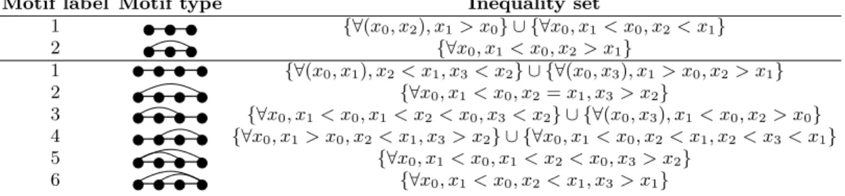
• Trivially, there is a total ofN−nmotifs (which can be the same motifs or not) within each VG/HVG. • Each motif is a subgraph of the original VG/HVG. Moreover, HVG motifs are outerplanar and have a trivial Hamiltonion path, thus HVG motifs are also HVGs [21]. As a result, there are only 6 admissible motifs of size 4, and 2 admissible motifs of size 3 (see table I for an enumeration).
• Computational complexity: Computing motifs in both VG and HVG is extremely efficient. If instead of exploring the motif occurrence in the structure of the adjacency matrix, one directly examines the set of inequalities reported in table I, one directly has an algorithm that runs inlineartimeO(N) for HVG motifs. A similar complexity is found for VG motifs [31].
As is done traditionally with network motifs [7], we can compare VG/HVGs associated to different time series and dynamics by comparing the relative occurrence of each motif inside a VG/HVG. In order to do that, we introduce the extension to the VG/HVG realm of a significance profile:
Definition (VG/HVG motif profile Zn). Let p be the total number of admissible VG/HVG motifs with n-nodes. Assign to each of these pmotifs a label from
0 1 2 3 4 5 6 7 8 9 10 11 12 13 14 15 16 17 18 19 20 0 0.2 0.4 0.6 0.8 1
b)
a)
0 1 2 3 4 5 6 7 8 9 10 11 12 13 14 15 16 17 18 19 20 0 0.2 0.4 0.6 0.8 1FIG. 1: (Color online) Schematic of two families of visibility algorithms. (a): Natural Visibility Algorithm applied to 20 data points of a periodic time series (top) and the corresponding Visibility Graph (VG) (bottom); each datum in the series corresponds to a node in the graph and two nodes are connected if their corresponding data heights show mutual visibility (see the text). (b): Horizontal Visibility Algorithm applied to the same series (top) and the corresponding Horizontal Visibility Graph (HVG) (bottom); each datum in the series corresponds to a node in the graph and two nodes are connected if their corresponding data heights show horizontal visibility (see the text).
1 to p(that is, choose an ordering for the motifs). The motif assigned with the label i will be called a type-i motif. Then, we define the n-node VG/HVG motif significance profile Zn (or simply HVG motif profile) of
a certain time series of size N as the vector function
Zn : n ∈ N → [P1n, . . . ,Pnp] ∈ [0,1]p whose output is a
vector ofp components, where the i-th component, Pni,
is the relative frequency of the type-imotif. Several technical comments are in order:
• First, since Zn aren-dimensional real vectors, any Lpnorm induces a natural similarity measure
(dis-tance) between two graphs.
• Second,Zn has, by construction, unitL
1-norm, as Pp i=1|P n i|= Pp i=1P n i = 1.
• Third, note that if one considers dynamical pro-cesses instead of individual time series, then the estimated relative frequencies Pn
i for an individual
realization of the dynamical process converge for in-finitely long series to the probabilities of type-i mo-tif associated to the process. For the momo-tif profile to be a well-defined feature of a certain dynamical process, it needs to be self-averaging. We check this property by estimatingZn for an ensemble of real-izations of the process, computing the mean hPnii
and standard deviationph[Pni]2i − hPnii2over this
ensemble, and checking that the standard deviation is small (meaning that a single realization provides a good description of the average behaviour). As we will show below, both VG and HVG motif pro-files have very good self-averaging properties. In any case, for every dynamical process considered
in this work, instead of Pni we compute hP n ii and
p
h[Pni]2i − hPnii2, but for readability, from now on
we will drop the h·i for the elements of the motif profile, as we found that for the size of the series used in the numerical analysis, p
h[Pn
i]2i − hP n ii2
was very small and hencePn
i ≈ hPnii.
• Fourth, note at this point that the definition of the VG/HVG motif profile is different from standard profiles (significance profile, subgraph ratio profile) defined in the literature [7], as in the latter case, they make use of a null model (ensemble of ran-domised networks) to appropriately normalise each frequency. The rationale for this normalization is that one wants to compare motif statistics across very different networks (with different sizes and de-gree sequences), so variations in the motif relative frequencies only due to size effects need to be re-moved to be able to correctly compare across dif-ferent networks. The reader will quickly come to the conclusion that, in the context of VG/HVG, the null model is not a randomised ensemble of the graph under study (which would not yield a VG/HVG with high probability), but on the con-trary, it should be the VG/HVG of a randomisation of thetime seriesunder study. In other words, nor-malisation in the case of VG/HVG profiles should deal with the motif statistics of uncorrelated ran-dom series (i.i.d. white noise or surrogate series that preserve certain structures) with similar prob-ability densities than the series under study. In the next section we will prove that, in the case of HVGs (which will be the family of visibility graphs under study), such null model has a universal motif pro-file, independent of the probability density of the
−3 −2 −1 0 1 2 3 4
x(t)
Gaussian i.i.d. 0 0.2 0.4 0.6 0.8 1x(t)
fully chaotic logistic map
0 20 40 60 80 100 −1 −0.5 0 0.5 1 1.5
t
x(t)
noisy fully chaotic logistic map
FIG. 2: (Color online)Sample time series from (a) i.i.d. Gaus-sian white noise, (b) fully chaotic logistic map, and (c) fully chaotic logistic map polluted with a certain amount of extrin-sic white noise are shown for illustrative purpose. Visibility graph motifs can be extracted from these series to reveal dif-ferences in their intrinsic structure.
i.i.d. process. Therefore, it is not necessary in this case to normalise each profile accordingly as this would only yield a trivial, constant rescaling. For illustration purposes, let n = 4, and consider two different dynamical processes: (i) white Gaussian noise described by the map xt = ξ, where ξ are independent
and identically distributed (i.i.d.) Gaussian random vari-ablesξ∼ N[0,1], and (ii) chaotic dynamics given by the fully chaotic logistic map xt+1 = 4xt(1−xt). In order
to estimate the probability of appearance of each of the motifs, we have generated a time series of size N = 104
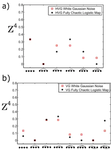
data for both processes (sample time series can be seen in the top panels of figure 2), and we have computed the relative frequencies of each motif. Results, averaged over an ensemble of 100 realizations, are shown in figure 3
(er-a)
0 0.1 0.2 0.3 0.4 0.5 0.6 0.7 0.8HVG White Gaussian Noise HVG Fully Chaotic Logistic Map
Z
4
Z
4
0 0.1 0.2 0.3 0.4 0.5 0.6 0.7 0.8VG White Gaussian Noise VG Fully Chaotic Logistic Map
b)
FIG. 3: (Color online) 4-node motif profiles Z4 associated
to Gaussian white noise (red squares) and to a fully chaotic logistic map (black stars) extracted respectively from HVG (panel a) and VG (panel b). Each dot represents the rela-tive frequency of a given motif, averaged over an ensemble of 100 realizations of each process (time series ofN = 104 data per realization). Standard deviations of each motif relative frequency over the ensemble are plotted as error bars, which are not visible as error bars fall inside the symbols. We con-clude that these motifs can be used to distinguish between deterministic and stochastic dynamics.
ror bars describing the ensemble standard deviation are contained inside the symbols); in panel (a) we plot the HVG motif profile, whereas in panel (b) we plot the VG profile. As we can see, in every case the type-II motif is absent. The simple reason is that this profile is ab-sent for irregular (aperiodic) real-valued time series, by construction (see table I).
For the chaotic process, some other motifs are absent: this is related to forbidden patterns arising in chaotic dynamics. More importantly, in both panels, the average relative frequency of some motifs seems to be different for both dynamical processes, enabling the possibility of using both HVG and VG motif profiles to distinguish amongst different dynamical origins. From now on we will focus our motif analysis on the horizontal visibility graphs (HVG) alone, and comparison with the VG case is left for future work [31]. In the next section we advance
a theory to compute the motif profile Zn in an exact way for different classes of dynamical systems. We will confirm that HVG motifs can indeed distinguish several kinds of dynamics, and we will explore how to build on this peculiar property for feature-based classification.
III. THEORY
In order to numerically explore and compute the fre-quency of each HVG motif, one can generate the HVG associated to a given time series and count the presence of each motif directly from the adjacency matrix. How-ever, in this section we will show that it is not necessary to do that as, via the zero-order terms of a diagram-matic expansion recently advanced [22], we can also work out the motif occurrence directly from the exploration of the time series, that enables motif computation in linear time. This will allow us to build a theory by which the motif profiles can be computed exactly for a large set of classes of dynamics that fulfil certain properties. Let us consider a dynamical process H:R→Rwith a smooth
invariant measuref(x) that fulfils the Markov property. That is, from a probabilistic point of view, conditional probabilities fulfil f(xn|xn−1, xn−2, . . .) = f(xn|xn−1),
where f(xn|xn−1) is the transition probability
distribu-tion (note that this concept has a clear meaning in ran-dom dynamical systems, whereas for deterministic sys-tems, say maps xt+1 = H(xt), the Markov property is
also trivially fulfilled with f(x2|x1) = δ(x2− H(x1)),
where δ(x) is the Dirac-delta distribution). The key el-ement is that for these processes, each HVG motif has a probability of appearance as a subgraph that can
di-rectly be computed as the measure of aset of ordering inequalities that take place in the time series. For in-stance, forn= 3 andn = 4, probabilities associated to the appearance of a certain motif are based on integrals of the form: Z f(x0)dx0 Z f(x1|x0)dx1 Z f(x2|x1)dx2 (1) forn= 3, and Z f(x0)dx0 Z f(x1|x0)dx1 Z f(x2|x1)dx2 Z f(x3|x2)dx3 (2) for n = 4. The range of integration and the shape of the conditional probabilities are particular for each mo-tif and each process, respectively. First, the range of integration fully determines the motif. In table I we de-pict the conditions in the time series that have to be ful-filled amongnconsecutive datax0, x1, . . . , xn−1 to yield
a certain motif of sizen in the HVG, for n = 3,4 (ex-tension to arbitrary n is easy but gets cumbersome as nincreases). It can be proved quite easily that a given motif appears in an HVG if and only if these ordering restrictions are fulfilled in the time series. These restric-tions directly translate in the integration range of the probabilities, we illustrate this principle in an example. The first motif, Z4
1, according to table I is guaranteed
when 4 consecutive valuesx0, x1, x2andx3are such that {∀(x0, x1), x2 < x1, x3< x2} ∪ {∀(x0, x3), x1 > x0, x2 >
x1}. Accordingly, ifx∈[a, b]⊂R, the probability of this
event is Z41≡P41= Z b a f(x0)dx0 Z b a f(x1|x0)dx1 Z x1 a f(x2|x1)dx2 Z x2 a f(x3|x2)dx3+ Z b a f(x0)dx0 Z b x0 f(x1|x0)dx1 Z b x1 f(x2|x1)dx2 Z b a f(x3|x2)dx3. (3)
Analogous expressions can be found for the rest of the probabilities that form the motif profile Z. These terms are nothing but the contributions to the degree distri-bution at zero-order from a diagrammatic expansion in the number of hidden nodes [22]. From a geometric point of view, the first motif will not appear in fast fluctuating signals and hence deals with the degree of smoothness of a time series at short (order n) scales, whereas the other motifs deal with certain fluctuation shapes. Accordingly, in those processes where the degree of smoothness can vary -such as in fractional Brownian motion, where the smoothness of the signal increases with the Hurst exponent- we would expect
that the first motif is particularly informative, whereas for fast-fluctuating series we expect this motif to be less informative. Integrals accounting for the probabilities are easy to deal with; in several cases these are exactly solvable, and in general one can solve them up to arbitrary precision with any symbolic programming software. In what follows we determine the motif profiles for i.i.d. (white noise), coloured noise with exponentially decaying correlations, and deterministic chaos (fully chaotic logistic map). We show thatZ4 capture enough
information to easily distinguish different processes and thus represent excellent features for series classification.
Motif label Motif type Inequality set 1 {∀(x0, x2), x1 > x0} ∪ {∀x0, x1< x0, x2< x1} 2 {∀x0, x1< x0, x2> x1} 1 {∀(x0, x1), x2< x1, x3< x2} ∪ {∀(x0, x3), x1> x0, x2> x1} 2 {∀x0, x1 < x0, x2=x1, x3> x2} 3 {∀x0, x1< x0, x1< x2< x0, x3 < x2} ∪ {∀(x0, x3), x1< x0, x2> x0} 4 {∀x0, x1> x0, x2< x1, x3> x2} ∪ {∀x0, x1< x0, x2< x1, x2< x3< x1} 5 {∀x0, x1< x0, x1< x2< x0, x3> x2} 6 {∀x0, x1 < x0, x2< x1, x3> x1}
TABLE I: Enumeration of all 3 and 4-node motifs. Each motif can be characterized according to a hierarchy of inequalities in the associated time series. Note that for real-valued aperiodic dynamics the type-II 4-node motif has a null probability of occurrence as the probability that two data in the time series repeat vanishes almost surely (if, on the other hand, the series only take values from a finite set then this motif has a finite probability). For the rest, the probability of each motif reduces to the measure of the set of inequalities (see the text).
Relation with ordinal patterns. At this point it is important to highlight the relation between the probabil-ity of occurrence of a given HVG motifs and the proba-bility of occurrence of so called ordinal patterns [27, 30]. In the theory proposed by Bandt and Pompe in[27] for the case of the embedding dimension equal to 4 one pro-ceeds to map each local time series segment of size 4 into an ordering symbol of 4 letters from the alphabet {0,1,2,3} (where the largest value maps to the letter 0, the second largest to 1, the third largest to 2, and the smallest to 3). There are 4! = 24 permutations, defin-ing 24 symbols (ordinal patterns) whose frequencies are then counted to measure the so-called permutation en-tropy that acts as a complexity measure of the series [27]. Interestingly, the probability of occurrence of each HVG motif indeed reduces to the probability of occur-rence of a set of possible ordinal patterns (this is no longer the case for VG motifs [31]). For instance, Z4 1
is the probability of finding any of the ordinal patterns 0123,1023,1203,1230,2103,2130,2310,or 3210, and sim-ilarly the rest of the motif probabilities can be linked to the probability of appearance of different sets of ordi-nal patterns. Accordingly, HVG motifs indeed induce a particular partition of the set of ordinal patterns. The HVG motif profile is thus intimately linked with the so called permutation spectrum [29] that accounts for the histogram of ordinal patterns.
A. i.i.d.
Let us start by considering time series generate by i.i.d. uniform random variables ξ ∼ U[0,1]. In this case we have a = 0, b = 1, f(x) = 1 andf(x|y) =f(x)∀y, and simply enough, probabilities defined by eqs. 1 and 2 eas-ily factorize. According to table I, after a little bit of calculus we find Z3= 2 3, 1 3 ; Z4= 8 24,0, 6 24, 6 24, 2 24, 2 24 (4) Note that these results are in perfect quantitative agreement with numerics performed for finite size series
(left panel of figure 3); we will show in the next sub-section that results for finite series converge quite fast to the (asymptotic) theory as the series size increases. Interestingly, results indeed coincide despite the fact that the theoretical values were computed for uniform
white noise (f(x) = 1), while the numerics in figure 3 were performed onGaussian white noise (where f(·) is the Gaussian function). This suggests that i.i.d. may have a universal HVG motif profile, indeed independent off(·). We now state and prove a theorem that actually guarantees this result.
Theorem 1. Consider a bi-infinite series of i.i.d. random variables extracted from a continuous distribu-tionf(x) with support (a, b), wherea, b∈R. Then the probability of findingn-node HVG motifs (withn= 3,4) follows eq. 4, independently of the shape off(x).
Proof. The proof is a constructive one. We only give here the explicit proof for P41, as the proof for
the rest of probabilities follow analogously. We rely on the cumulative distribution function F(x), defined as Rx
a f(x
0)dx0 =F(x), with properties F(a) = 0, F(b) = 1
and f(x)Fn−1(x) = dF n(x) ndx . (5) We have P41= Z b a f(x0)dx0 Z b a f(x1)dx1 Z x1 a f(x2)dx2 Z x2 a f(x3)dx3+ Z b a f(x0)dx0 Z b x0 f(x1)dx1 Z b x1 f(x2)dx2 Z b a f(x3)dx3
Using the properties ofF(x), the first term above is then Z b a f(x0)dx0 Z b a f(x1)dx1 Z x1 a f(x2)dx2 Z x2 a f(x3)dx3= Z b a f(x0)dx0 Z b a f(x1)dx1 Z x1 a f(x2)F(x2)dx2= Z b a f(x0)dx0 Z b a f(x1) F2(x 1) 2 dx1= Z b a f(x0) 6 dx0= 1 6,
and analogously for the second term, Z b a f(x0)dx0 Z b x0 f(x1)dx1 Z b x1 f(x2)dx2 Z b a f(x3)dx3= Z b a f(x0)dx0 Z b x0 f(x1)(1−F(x1))dx1= Z b a f(x0) 1 2 −F(x0) + F2(x0) 2 dx0= F(x0) 2 − F2(x 0) 2 + F3(x 0) 6 b a = 1 6, (6)
hence P41 = 2/6 = 8/24, coinciding with the result for
uniform and Gaussian series, and being independent of f(x). The rest of the elements in Z4 are computed
analogously.
As a matter of fact, the independency from f(x) can be trivially extended for an arbitrary size of the motif n. This is intuitive so we only give here the strategy of a proof. The main ingredient which is required for this independency to hold ∀n is that the limits of the n-th integral are either the extremes of the distribution support a, b (where the cumulative distribution F(x) take the constant values 0 and 1 respectively, and independently of f(x)), or other variables x0. . . xn−1.
In this latter case, one can use iteratively the prop-erty in eq. 5 to solve these integrals up to the last one (in x0), whose range is always (a, b) and where
F(a) = 0, F(b) = 1 can be finally applied, to give a result which will not depend on the precise shape off(x). According to theorem 1, Gaussian, uniform, power law, etc, uncorrelated random series all have the same HVG motif profiles. As a byproduct, for any kind of sufficiently long time series {xt}Nt=1 where xt ∈ f(x)
and f(x) is continuous, if we randomize (shuffle) the time series, the motif profile of the randomized series is equal to eq. 4. This is the reason why, at odds with the standard definition of a network’s motif profile, for HVGs we don’t need to rescaleZin any way to be able to compare across different time series and dynamical process.
Another notable consequence of theorem 1 is that it guar-antees that series for whichZ4 differ (even in the case of
sufficiently long time series) from eq. 4 are not uncor-related random series. This suggests a simple test for randomness [15]. For instance, one can use a Pearson’s χ2hypothesis test, where the null hypothesis is that the
observed time series ofN data is random and uncorre-lated (white noise). The test statistic is then
χ2= (N−n) p X i=1 [P4 i(observed)−P4i(i.i.d.)]2 P4i(observed) (7)
χ2 upper-critical values with p−1 degrees of freedom,
for p = 6 (n = 4) are 11.07 and 15.086 at the 95% and 99% significance level (meaning that values of theχ2 larger than 11.07 suggest that the observed series is not random at the 95% significance level). More rigorously, as type-II motif is forbidden for aperiodic dynamics, we have onlyp= 5 different motifs of sizen= 4, so theχ2
upper-critical values should be considered for 4 degrees of freedom: 9.49 (95%) and 13.28 (99%).
B. Deterministic chaos: fully chaotic logistic map
As previously stated, deterministic mapsxt+1=H(x)
are indeed Markovian, and for these situations the con-ditional probability is simplyf(x2|x1) =δ(x2− H(x1)),
whereδ(x) is the Dirac-delta distribution. Therefore eqs. 1 and 2, combined with inequality sets given in table I can be used to compute the motif profiles for different deterministic processes. In these cases, one has to deal with simple integrals of the form
Z q p δ(x−y)dx= 1 y ∈[p, q] 0 otherwise (8)
While in principle any deterministic process can be stud-ied, we are interested in complex signals, so we focus on irregular, aperiodic dynamics. As a paradigmatic case, we tackle the fully chaotic logistic map
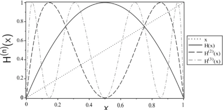
H(x) = 4x(1−x), x∈[0,1], f(x) = 1 πpx(1−x). In this case,f(x) is the invariant measure that describes in a probabilistic way the average time spent by a chaotic trajectory in each region of the attractor. Let us start by consideringZ3:= ( P31,P32), for which P31= Z 1 0 f(x0)dx0 Z 1 x0 δ(x1− H(x0))dx1 Z 1 0 δ(x2− H2(x0))dx2, P32= Z 1 0 f(x0)dx0 Z x0 0 δ(x1− H(x0))dx1 Z 1 x1 δ(x2− H2(x0))dx2.
According to property in eq. 8, the Dirac-delta integrals only have the effect of shrinking the range of integration
FIG. 4: Cobweb plot of the iterates of the fully chaotic logistic mapH(x) = 4x(1−x).
of x0. For instance, for P31, the integral in x1 requires H(x0)> x0, whereas the integral in x2 simply requires H2(x
0) ∈ [0,1]. While the latter inequality is fulfilled
for all x0 ∈ [0,1] (and thus has no effect), the former
one requires x0 ∈ [0,3/4]. This can be easily seen from
the cobweb plot of H(x) and its iterates (see figure 4): H(x)> xforx∈[0,3/4]. Altogether,
P31=
Z 3/4
0
f(x0)dx0= 2/3
On the other hand, motif normalization imposes P32 =
1/3. The same result is obviously found if we computeP32
explicitly: in this case the integral inx1requiresH(x0)<
x0, which holds when x0 ∈ [3/4,1], and the integral in
x2 requires H2(x0) > x1 ↔ H2(x0) > H(x0). Looking
at the cobweb plots, this final condition is met in two subintervals, so the intersection with the first condition yields a final intervalx0∈[3/4,1], for which
P32=
Z 1
3/4
f(x0)dx0= 1/3,
as expected. These results coincide with those found for i.i.d. series, meaning that Z3 doesn’t capture enough structure to distinguish both processes. Let us proceed in an equivalent way to compute Z4 = (
P41, . . . ,P46).
It becomes evident that integrals associated to xn deal
with the cobweb plots of H(x),H2(x), . . . ,Hn(x).
Ac-cordingly, these integrals are ultimately related with the structure of fixed points of Hn(x), and with the
solu-tions of equasolu-tions of the formHr(x) = Hs(x) for some
r and s. We only have algebraic closed expressions for the fixed points of H(x) → {0,3/4} and H2(x) → {0,5− √ 5 8 ,3/4, 5+√5 8 }(forn≥3,H n(x) is a polynomial of
order larger or equal to 6 and according to Abel-Ruffini’s theorem, the set of fixed points does not have in gen-eral an algebraic expression, however we can compute them up to arbitrary precision). Other values of interest include the roots of H3(x) = H2(x), and specially the
largest onex= 1/2 +√3/4.
Let us show how to compute one of these motif probabil-ities. For instance,
P45= Z 1 0 f(x0)dx0 Z x0 0 δ(x1− H(x0))dx1 Z x0 x1 δ(x2− H2(x0))dx2 Z 1 x2 δ(x3− H3(x0))dx3 (9) which reduces to P45= Z q p f(x0)dx0,
where [p, q] can be hierarchically obtained as: H(x0)< x0∩[0,1]⇒x0∈[3/4,1]; H2(x 0) < x0 ∩ H2(x0) > H(x0)∩ [3/4,1] ⇒ x0 ∈ [5+ √ 5 8 ,1]; H3(x 0) > H2(x0)∩[5+ √ 5 8 ,1] ⇒ x0 ∈ [xp,1], where xp
is the second largest root fulfillingH3(x
p) =H2(xp), i.e xp= 1/2 + √ 3/4. Altogether, P45= Z 1 1/2+√3/4 1 πpx0(1−x0) dx0= 1 πBh1 2+ √ 3 4 ,1 i 1 2, 1 2 =1 6(= 4/24)
(where B is the incomplete Beta function), which is indeed quite different from the result found for i.i.d.,
P45(i.i.d.) = 2/24.
Similar arguments can be used to obtain analytically the rest of probabilities (explicit computations are put in an appendix), finding Z3= 2 3, 1 3 ; Z4= 8 24,0, 4 24, 8 24, 4 24,0 (10) Comparing this set of motif probabilities with the re-sult for i.i.d. (eq. 4), we can conclude that Z4
distin-guishes the fully chaotic logistic map from a purely un-correlated stochastic process. Note, of course, that a sim-ilar derivation can be performed in other deterministic maps; in this sense the methodology is general (however one encounters problems when the attractor has a frac-tal dimension, and one needs to carefully choose a proper integration theory). These exact results are also in excel-lent quantitative agreement with numerics performed in finite series (left panel of figure 3), so convergence to the theory with series size is quite fast, enabling its use in
empirical cases. To be more precise, in the next subsec-tion we make a study of how fast results for short time series converge to the asymptotic theory as series size increases.
C. Convergence of finite series
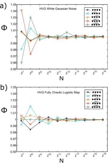
In order to be more precise about the convergence speed of finite-size numerics to the theory (which in rigour only holds for bi-infinite time series), we have com-puted for series of size N the numeral estimate Z4(N)
for both i.i.d. and the fully chaotic logistic map, and compare it with the asymptotic values Z4. Results are
plotted in figure 5, where we plot Φ(N) = hZ4(N)i/Z4
as a function of the series sizeN (the average is with re-spect to realizations). Results indicate that convergence to the asymptotic theory is already reached forN 104
(which is the conservative size that is used all over this work).
D. Stochastic processes with correlations
To round off the theory section, and to explore how results deviate from i.i.d. for correlated stochastic pro-cesses, we consider coloured noise with exponentially de-caying correlations as described by the AR(1) process:
( x0=ξ0 xt=rxt−1+ p (1−r2)ξ t, t≥1 (11)
whereξt∼ N(0,1) is Gaussian white, and r, 0< r < 1
is a parameter that tunes the correlation. The auto-correlation function C(t), which describes the correla-tion of the posicorrela-tion atxt0 andxt0+tdecays exponentially C(t) =e−t/τ, where the characteristic timeτ = 1/ln(r).
In the limitr→0, the correlations vanish and the pro-cess reduces to a white noise signal. The limitr→1 is more delicate, but intuitively in this limit the process gets completely correlated and tends to be constantxt+1=xt
∀t.
This is a family of models parametrized by the coeffi-cient r. For 0< r < 1, these models are indeed Gaus-sian, Markovian and stationary, with a probability den-sityf(x) and transition probability f(x2|x1) are
f(x) =exp(√−x2/2) 2π f(x2|x1) = exp[−(x2−rx1) 2/(2(1−r2))] √ 2π(1−r2)
respectively. Since x are Gaussian variables they can vary in (−∞,∞). We focus on Z4 that we know gave
good discriminatory results between i.i.d. and chaos. For illustration, the first element reads
P41= Z ∞ −∞ e −x20 2 √ 2πdx0 Z ∞ −∞ e −(x1−rx0 )2 2(1−r2 ) p 2π(1−r2)dx1 Z x1 −∞ e −(x2−rx1 )2 2(1−r2 ) p 2π(1−r2)dx2 Z x2 −∞ e −(x3−rx2 )2 2(1−r2 ) p 2π(1−r2)dx3+ Z ∞ −∞ e −x20 2 √ 2πdx0 Z ∞ x0 e −(x1−rx0 )2 2(1−r2 ) p 2π(1−r2)dx1 Z b x1 e −(x2−rx1 )2 2(1−r2 ) p 2π(1−r2)dx2 Z ∞ −∞ e −(x3−rx2 )2 2(1−r2 ) p 2π(1−r2)dx3 (12)
For any particular value ofr, these integrals can be eval-uated up to arbitrary precision using Mathematica [32]. In table Table II we report the theoretical values ofZ4(r)
forr∈[0.02−0.99]. These are in perfect agreement with numerical simulations performed on finite series of size N = 104 (ensemble averaged over 100 realizations) for
r ={0,0.1,0.3,0.5,0.7,0.9,0.99}, as shown in Figure 6. Asr >0 the profiles deviate from i.i.d. and thus, again, these features can easily distinguish between exponen-tially coloured and white noise.
IV. ROBUSTNESS
In the preceding section we have developed a general theory to compute explicitly the motif profile of HVGs associated to a given type of dynamics. We have ap-plied this theory to find theoretical expressions in the case of white and coloured noise as well as chaotic dy-namics, and have shown that these predictions perfectly match the results found in numerical simulations for rea-sonably short time series. The theory (which is exact in the limit of infinite size series) is thus correct also in the case of short time series. These are nonetheless only idealized models: empirical time series, however, even if they comply to a particular dynamical system are
usu-a)
HVG Fully Chaotic Logistic Map
b)
HVG White Gaussian Noise
27 28 29 10 11 12 13 14 0.95 0.96 0.97 0.98 0.99 1 1.01 1.02 1.03 1.04 1.05
N
15 16 2 2 2 2 2 2 2Φ
0.95 0.96 0.97 0.98 0.99 1 1.01 1.02 1.03 1.04 1.05 27 28 29 10 11 12 13 14N
15 16 2 2 2 2 2 2 2Φ
FIG. 5: (Color online) The measured frequency of appear-ance rescaled by its theoretical value Φ is plotted for each motif associated to Gaussian white noise (panel a) and to a fully chaotic logistic map (panel b) in function of the time series sizeN; results are averaged over 100 realisations. The curves oscillate with fast decreasing amplitude around the value 1 (for 29 the amplitude is less than 10−2) indicating
fast asymptotic convergence of the measured motif profile to the theoretical profile in both cases.
ally polluted with measurement noise. Therefore, before being able to apply this new technique to real world phe-nomena, we need to assess its robustness and reliability against noise contamination. To do that, we consider a situation where a chaotic time series is contaminated with different amounts of white noise, and explore the ability of Z4 to detect the chaotic signal. Formally, we pollute a chaotic signalx(t) with uniform white noise ξ(a) and thus construct a noisy chaotic signalY(t) such that
Yt=xt+ξ xt= 4xt−1(1−xt−1) ξ∼U[0, a], 0≤a≤1, (13)
whereatunes the noise power. The noise-to-signal ratio of the signal Yt is defined as N SR = σξ2/σ
2 Y (where r P41 P42 P43,P44 P45,P46 0.02 0.3370 0 0.2482 0.0833 0.04 0.3406 0 0.2464 0.0833 0.06 0.3443 0 0.2446 0.0832 0.08 0.3478 0 0.2429 0.0831 0.1 0.3514 0 0.2412 0.0830 0.2 0.3690 0 0.2333 0.0822 0.3 0.3862 0 0.2260 0.0809 0.4 0.4030 0 0.2192 0.0793 0.5 0.4196 0 0.2130 0.0772 0.6 0.4359 0 0.2072 0.0748 0.7 0.4521 0 0.2018 0.0722 0.8 0.4681 0 0.1967 0.0692 0.9 0.4841 0 0.1920 0.0660 0.95 0.4919 0 0.1897 0.0643 0.97 0.4945 0 0.1888 0.0636 0.99 0.4973 0 0.1879 0.1879
TABLE II: Theoretical values ofZ4(r) for the AR(1) process evaluated at different values of the coefficientr.
0 0.1 0.2 0.3 0.4 0.5 r=0 r=0.1 r=0.3 r=0.5 r=0.7 r=0.9 r=0.999 theory
Z
4
FIG. 6: (Color online) HVG significance profileZ4for AR(1) processes described by eq.11, for different values of the corre-lation coefficientr. When rincreases the appearance proba-bility of motif of type-I increases while the rest of probabilities decrease. This is simply due to the fact that finding constant sequencesxt+3 =xt+2=xt+1 =xt becomes more probable asr increases.
σ·2 denotes the variance of signal ·), thus N SR will increase monotonically witha. ForN SR1, the noise contamination is small. Any technique that is able to distinguish Y(t) and ξ(t) for increasing values of N SR is said to be robust to noise. ForN SR= 1 the levels of the signal and the noise contamination are comparable and for N SR > 1 the underlying chaotic signal is effectively hidden. Of course, when a reaches a certain value it won’t be possible any more to distinguish the underlying chaotic nature of the time series by looking at the motif profile. To estimate this threshold we can use two different tests:
• The first test makes use of the (L1) distance in
|Z4(Y)−Z4(iid)|. This is just a simple, motif-based similarity metric between two graphs, that we use here to measure the similarity between two series. Ideally, the threshold of distinguishability is the smallest value of a for which d(a) = 0. How-ever, in practice, as we are dealing with finite size series, there will always be a small uncertainty as-sociated to small finite-size deviations from the the-ory. That is, if one estimates the Z4(iid) with an
ensemble average of m realizations of a finite ran-dom time series ofN data, then for each element in the profile, the standard deviation of the estimate
P4i will be a finite value (that converges to zero as
N and m increases). We defineσ(Z4(iid)) as the
vector where the i-th term is such standard devia-tion, for the same values of N and m used in the analysis of Y(t). Then, we define the uncertainty threshold a∗ as the smallest value of a such that d(a) ≤ |σ(Z4(iid))| (intuitively, a∗ is the smallest
value for which we don’t know if the difference in the motif profile between the empirical results and the theory are due to the fact that there is a chaotic signal underlying the process, or just due to finite size effects).
• The second possibility is to use a Pearson’s χ2
hy-pothesis test such as equation 7 with 4 degrees of freedom, where the null hypothesis is thatY(t) (the observed series) is just white noise (no hidden sig-nal). In this latter case, we are not taking into account the deviations associated to finite size ef-fects in the profile of i.i.d., though. If χ2 < 9.49, then we can’t reject the null hypothesis at the 95% significance level: this is the limit of what we could call certain distinguishability.
For each value of the parameter a, we have simulated a time series of N = 104 steps from the process Y(t),
and results were ensemble averaged over m= 100 reali-sations. In panel (b) of figure 7, we plot the motif profile as a function of a. It is interesting to observe that the probabilities which vary most withaare related to types III, IV, V and VI, while type-I seems to maintain ap-proximately the same rate of appearance (we will show later that this is not always the case). In the panel (a) of the same figure we plot d(a). As expected, d(a) is a monotonically decreasing function of a, and we find a∗ ≈1. Remarkably, this corresponds to a value of the noise to signal ratio N SR ≈ 2.67. This is indeed con-firmed by the Pearson χ2 test, where we found that the
limit for confidently rejecting the null hypothesis -certain distinguishability- isa≈1 (i.e. N SR≈2.67). These re-sults prove thatZ4is indeed an extremely robust feature with respect to measurement noise contamination, hence useful for applications.
V. PRINCIPAL COMPONENT ANALYSIS
According to the last sections, we can conclude that the HVG Z4 is an informative feature of complex
dy-namics. Here we summarise and gather the findings on i.i.d., fully chaotic logistic maps (with and without noise contamination) and coloured noise, and we complement those with additional chaotic maps (Ricker’s map, Cubic map, Sine map). Each process is described by the six dimensional vector Z4 (although in practice this space
is 5-dimensional as P42 = 0). As this representation is
obviously not very convenient for readability, we have projected each point into a 2-dimensional space spanned by the principal components of the data. We recall that Principal Component Analysis (PCA) [33] is a common statistical procedure to perform dimensionality reduction on data. It uses an orthogonal transformation to project our set of observations, originally described in R6 -where each direction describes the probability
of occurrence of a given motif, this being possibly correlated among observations- into a lower dimensional subspace spanned by the so called principal components, obtained from the eigenvectors of the dataset covariance matrix. These particular directions are such that (i) they are orthogonal, (ii) the first principal component has the largest possible variance (that is, accounts for as much of the variability in the data as possible), and each succeeding component in turn has the highest variance possible under the constraint that it is orthogonal to (i.e., uncorrelated with) the preceding components. If the data can be efficiently projected in a lower dimen-sional space, then the eigenvalues associated to each of the principal components sum up a large percentage of the data variability. In that case, the projection is said to be faithful, and constitutes an accurate description of the data.
To summarise, the following processes have been consid-ered (for all of them, we have estimatedZ4 from a time series of N = 104 points, and have averaged this over 100 realisations):
• White noise (i.i.d.) with Gaussian, exponential, uniform and power-low probability densities. • Chaotic maps, in particular: Fully chaotic
logis-tic map xt+1 = 4xt(1−xt), Ricker’s map xt+1 =
20xte−xt, Cubic mapxt+1= 3xt(1−x2t), Sine map
xt+1= sin(πxt)
• Noisy logistic map witha={0.2,0.4,0.6,0.8,1.0} • Coloured noise forr={0.1,0.3,0.5,0.7,0.9,0.99} The projection into the space spanned by the first two principal components is shown in figure 8. Interestingly, these first two components capture about 98.3% of the variability of the set of variables{Z4}. This means that motif probabilities are indeed highly correlated, and as few as two real numbers per time series seem already
a)
b)
0 0.2 0.4 0.6 0.8 1 1.2 1.4 1.6 1.8 2 0 0.05 0.1 0.15 0.2 0.25 0.3 0.35d
a
d uncertainty threshold 0 0.1 0.2 0.3 a=0 a=0.2 a=0.4 a=0.6 a=0.8 a=1 white noiseNSR
0 0.11 0.43 0.96 1.71 2.67 3.84 5.22 6.83 8.64 10.66Z
4
FIG. 7: (Color online) Robustness of motif profiles for chaotic series (fully chaotic logistic map) polluted with white noise. Panel a): by increasing the amount of extrinsic noise (parameterised bya) the distance in motif space between the noisy chaotic signal and white noise decreases (see the text). The method is extremely robust as one can distinguish the noisy chaotic signal from pure white noise up to a noise-to-signal ratioN SR≈2.67. Panel b): the 4-node motif profile of the noisy chaotic signal
Ytfor different degrees of noise contamination (a). Motifs III, IV, V and VI are the most informative as they concentrate most of the profile variability.
−
1
−
0.8
−
0.6
−
0.4
−
0.2
0
0.2
0.4
0.6
0.8
−
0.6
−
0.4
−
0.2
0
0.2
0.4
0.6
S
e
co
n
d
C
o
m
p
o
n
e
n
t
(1
5
.9
%
)
First Component (82.4%)
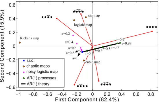
i.i.d. chaotic maps noisy logistic map AR(1) processes AR(1) theory r=0.99 r=0.9 r=0.7 r=0.5 r=0.3 r=0.1 a=1 a=0.2 a=0.8 a=0.6 a=0.4 Ricker's map cubic map logistic map sin mapFIG. 8: (Color online) 2-dimensional projection obtained via Principal Component Analysis onZ4for time series generated from
different deterministic and stochastic processes: different white noise series respectively with Gaussian, exponential, uniform and power low (blue squares), chaotic maps (brown diamonds), noisy logistic map for different levels of contamination (purple dots) and different stochastic correlated AR(1) processes (green triangles). The relative weight of each motif in this projection principal components is also plotted using red solid axes.
enough to describe them. The patterns related to the different processes in this 2-dimensional component space help visualize some of the results previously found and make interesting considerations:
• All the i.i.d. processes have the same coordinates
in the 2-dimensional space which do not correspond to the coordinates of any other class of processes considered. Indeed according to the theory, i.i.d. processes share the sameZ4.
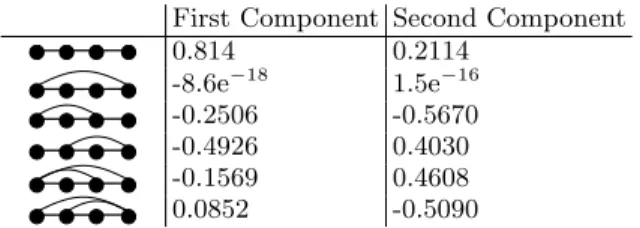
projec-First Component Second Component 0.814 0.2114 -8.6e−18 1.5e−16 -0.2506 -0.5670 -0.4926 0.4030 -0.1569 0.4608 0.0852 -0.5090
TABLE III: Weights of each motif in the 2-dimensional pro-jection of the set of all dynamical processes analysed (i.i.d. white noise, coloured noise with exponentially decaying cor-relations, chaotic maps, noisy chaotic logistic map).
tion of each motif in this new basis (see also table III) and give an idea of which motif types are more related to different processes, thus helping to in-terpret a particular trajectory in this space, as a given process changes. For instance coloured noise which interpolates between white noise (r→0) and a constant series (r → 1) projects into a straight line-like trajectory, departing from the i.i.d. co-ordinates and following the direction where type-I motif increases as rincreases. Analogously, as the noise level aincreases the noisy logistic map inter-polates between the fully chaotic logistic coordinate and i.i.d. following a specific path.
• The distance in this space between i.i.d. and the (a= 1)-noisy logistic map gives us a rough idea of the distinguishability or coarse-graining distance, a lower bound below which any two processes cannot be distinguished.
We conclude that Z4 is a highly informative and robust
feature, which in principle could be used to assess simi-larities and differences across empirical complex signals. To test this hypothesis, in the final section we will ex-plore this idea and will show that clustering of complex physiological processes is possible with this simple fea-ture.
VI. UNSUPERVISED LEARNING:
DISENTANGLING MEDITATIVE FROM OTHER RELAXATION STATES USING HVG MOTIF PROFILES FROM HEART RATE TIME SERIES
It is well-known that meditation has a measurable ef-fect on well-being. In particular, neuroscience has shown that meditation promotes EEG high-amplitude gamma synchronisation [34], or increases sustained attention [35] among others effects on the brain [36]. In this final sec-tion we explore, via a HVG motif profile analysis, if one can distinguish purely meditative states from gen-eral states of relaxation by only looking at a single phys-iological indicator: the heart rate series [37, 38]. This analysis is based on experiments performed in a former publication [39]. Data are freely available online [40].
A. Data
Data are collected for five different groups of healthy subjects [39]:
• The first group of 4 subjects (two women and two men in the age range 20-52) wereexpertKundalini Yoga meditators. Their heart rate was recorded for approximately fifteen minutes before the Yoga practice (pre-meditative state) and for approxi-mately one hour during the breathing and chant-ing exercises (meditative state) (a total of 8 time series);
• The second group comprised 8 Chinese Chi Medi-tation practitioners, (five women and three man in the age range 26-35)relatively novice in the prac-tice. The heart rate of the subjects was recorded for approximately five hours during the pre-meditation (pre-meditative state) and for approximately one hour during the meditation session (meditative state)(a total of 16 time series).
To better compare the pre-meditation and meditation states, three healthy, non-meditating control groups were considered from a database of retrospective electrocardio-gram (ECG) signals:
• a spontaneous breathing group of 13 subjects (eight women and five men in the age range 25-35) during sleeping hours (general relaxation state) (a total of 13 time series);
• a group of 9 elite triathlon athletes (six women three men, age range 21-55) in the pre-race period during sleeping hours (general relaxation state) (a total of 9 time series);
• a group of 14 subjects (nine women and five men, age range 20-35) during supine metronomic breath-ing at 0.25 Hz (a total of 14 time series);
Sample time series from each group are plotted in fig-ure 9. In the original study the authors addressed the frequency spectra and observed prominent heart rate os-cillations in the time series recorded during the two med-itation practices with a peak in the range 0.025-0.35 Hz, and an overall variability of these series with respect to those from non-meditative states.
B. Unsupervised clustering based on HVG motif
profiles
The total dataset is made of a total of 60 time series (60 observations). A priori, we assume that each series is a different process. For each subject and state, we extract from the heart beat series the correspondingZ4
40 60 80 100 120 chi pre 40 60 80 100 120 chi med 40 60 80 100 120 yoga pre 40 60 80 100 120 yoga med 40 60 80 100 120 sleeping 40 60 80 100 120 metronomic breathing 40 60 80 100 120 athletes sleeping 0 200 400 600 Heart rate ( bpm) Heart rate ( bpm) Heart rate ( bpm) Heart rate ( bpm) Heart rate ( bpm) Heart rate ( bpm) Heart rate ( bpm) time (s)
FIG. 9: Sample heart rate time series from patients in medi-tative and non-medimedi-tative states.
As a first analysis, we only consider theexpert medita-tors (first group) performing two different tasks and we explore ifZ4 can disentangle the two tasks. Results are
shown in panel (a) of figure 10. In PCA space, we have 8 points scattered over the subspace spanned by the first two principal components. These aggregate more than 99% of the data variance and is thus a faithful projection. Interestingly, already a visual inspection clusters the 4 subjects in the meditative state (red circles, right hand side of the plane) from those in the pre-meditative state (green squares). A simplek-means algorithm [33] with k = 2 correctly distinguishes the two states by assigning different clusters to both states (a black dotted oval is depicted with the purpose of visualizing the result of thek-means clustering).
In a second step, we consider the second group, formed now bynoviceChi meditators before and during the prac-tice. We repeat the analysis in the panel (b) of figure 10. Again the first two principal components capture more than 99% of the variability of the motifs considered. The scores related to the first principal component are very close to the ones found for the Yoga data subset (see appendix). For this meditation technique however it is not that easy to perfectly distinguish pre-meditative from meditative state clusters: the partition obtained with the k-means algorithm with inputk = 2 (visualized by the black dotted line) contain ‘false meditators’ and ‘false non-meditators’. In order to quantify the performance of the clustering we use the so calledpurity coefficient [41] defined by: purity = n 1 m+n0n n1 m+n0m+n0m+n1n (14) where n1m is the number of meditators in the cluster 1, which is defined as the cluster where most of the meditators are found;n0
mis the number of meditators in
the cluster 0, which is defined as the cluster where most of the non-meditators are found (‘false non-meditators’); n1n is the number of non-meditators in the cluster 1
(‘false meditators’);n0
n is the number of non-meditators
in the cluster 0. Purity takes value in [0,1] and was measured for the different partitions reported in figure 10 (see table IV); in this case we found purity'0.83. Now, as in this experiment the subjects were inexperienced Chi meditators, it is plausible that some of them were not able to concentrate of perform the task adequately, what would put their motif profile mixed amongst the pre-meditative state subjects. As we can see in the figure, there is some evidence of finding the ‘false non-meditators’ intertwined among non-meditators, but not the ‘false meditators’ intertwined among meditators. We then perform the same analysis by considering data from the first two groups (Yoga group and the Chi group) altogether. Here we also aim at distinguishing meditative from pre-meditative states, however this is in principle much more delicate and problematic as we have different
d)
−1 −0.5 0 0.5 1 −0.2 −0.1 0 0.1 0.2 0.3 0.4 0.5 Second Component (8.5%) First Component (86.1%) chi pre chi med yoga pre yoga med sleeping athletes sleeping Cluster 1 Cluster 2 Centroidsc)
−1 −0.5 0 0.5 1 −0.5 −0.4 −0.3 −0.2 −0.1 0 0.1 0.2 0.3 0.4 Second Component (6.1%) First Component (93.1%) chi pre chi med yoga pre yoga med −1 −0.5 0 0.5 1 −0.4 −0.3 −0.2 −0.1 0 0.1 0.2 0.3 0.4 Second Component (6.8%) First Component (92.8%) yoga pre yoga meda)
−1 −0.5 0 0.5 1 −0.2 −0.15 −0.1 −0.05 0 0.05 0.1 0.15 0.2 Second Component (3.8%) First Component (95.4%) chi pre chi medb)
metronomic breathingFIG. 10: (Color online) 2-dimensional Principal Component space of Z4 extracted from heart rate time series of subjects
performing different tasks. (a) 4 Yoga meditators recorded during meditation (red dots) and during pre-meditation (green squares). Thek-means algorithm (black dotted line) correctly assigns each of the 8 observations into the correct cluster. (b) 8 Chi meditators recorded during meditation (magenta triangles) and during pre-meditation (blue reverse triangles). The
k-means algorithm correctly 12 out of 16 observations, however in this case subjects were novice meditators, hence clusters are not that well defined (see the text). (c) The two clusters found by thek-means algorithm correctly clusters the points related to Yoga meditation and Yoga pre-meditation, and 12 out of 16 points related to different Chi meditators (black dotted line). (d): although thek-means clustering (small panel on the top right) fails to precisely distinguish a cluster related to meditation from a cluster related to non-meditation, all the meditation points are surprisingly well separated from the all remaining points, on the right side of the plane.
subjects performing different tasks. The results are re-ported in panel (c) of Figure 10, and are consistent with the first two analysis conducted before. In PCA space, the first two principal components still capture more than 99% of the data variability (scores are reported in the appendix). k-means correctly clusters together most of the pre-meditative states and distinguishes them from the meditative states (Yoga and Chi-style), with purity= 0.75. There are two clear ’false non-meditators’ which seem to correspond to two novice Chi meditators that falsely fall in the non-meditation state despite they were supposedly performing meditation. The two ‘false meditators’ are not mixed among the meditators but placed in the boundary of the cluster, meaning that a
refined clustering algorithm would very likely do a better job. On the other hand, it is worth highlighting that meditators show lower scattering than non-meditators, and are placed at the right hand side of the plane. Among these, Chi meditators (the experienced subjects) appear even more towards the right hand side in the PCA plane. According to the motif scores (appendix), one can conclude that meditation promotes the onset of type-I motifs, that is to say, generates a relative decrease of high-frequency heart rate fluctuations.
Finally, in panel (d) of Figure 10 we show the results for the analysis of the whole data set (the projection in PCA space still gathers more than 94% of the data
variabil-Panel a variabil-Panel b variabil-Panel c variabil-Panel d
1 0.83 0.75 0.81
TABLE IV: Purity measures [41] of the k-means clustering analysis depicted in the four panels of figure 10: yoga medi-tators (panel a), chi medimedi-tators (panel b), yoga and chi med-itators (panel c) and all states (panel d).
ity). Here we have highly heterogeneous subjects per-forming totally different tasks, which somehow can be classified into ‘meditative’ and ‘non-meditative’ states. In the inset panel of the same figure, each observation is labelled according to the result of k-means (crosses for non-meditative and dots for meditative states). Despite the heterogeneity of subjects, the purity of the partition obtained is high ('0.81), and most of the observations associated to the meditative state concentrate towards the right hand side of the PCA plane (which, again ac-cording to the scores, corresponds to an overcontribu-tion of type-I motif). We conclude that meditative prac-tices leave a unique physiological fingerprint in the heart rate time series of its practitioners, which can be distin-guished from other relaxation techniques and states such as metronomic breathing or sleeping by using the HVG motif profile of each time series. This is a remarkable result, taking into account that this profile only consists of a vector of 6 numbers (actually 5 asP42 = 0) per
ob-servation.
VII. CONCLUSIONS
The theory of visibility graphs (VG and HVG) allows us to describe and characterise time series and dynamics using the powerful machinery of graph theory and network science. Here we have introduced the concept of Horizontal Visibility Graph (HVG) motifs, substructures present in the HVG of a time series, whose statistics have been shown to be informative about the time series structure and its underlying dynamics (comparison with VG motifs will be published elsewhere [31]). We have advanced a mathematically sound theory by which the motif profile of large classes of stochastic and deterministic dynamics can be computed exactly. Interestingly, under the HVG framework, graph motifs are in direct correspondence with ordinal patterns [27– 30]. This means, for instance, that the theory developed here can be exported to find rigorous results on the permutation entropy [28] and permutation spectra [29] of different dynamical systems. In the same vein, one could import concepts and ideas from ordinal patters to the context of visibility graphs. For instance, one can define an HVG motif entropy Sn = −n1PZni log(Z
n i)
and explore its similarities with permutation entropy. More generally, the relation (and possible equivalences) between ordinal pattern analysis (so called permutation complexity [28, 30]) and horizontal visibility graph analysis should be studied in more depth. We have
found that this graph feature is surprisingly robust, in the sense that it is still able to distinguish amongst different dynamics even when the signals are polluted with large amounts of measurement noise, what enables its use in practical problems. Despite the apparently difficult combinatorial interpretation of the visibility criteria, these latter results further suggest that HVG motifs are more than just an arbitrary partition on the set of ordinal patterns. As an application, we have tackled the problem of disentangling meditative from general relaxation states from the HVG motif profiles of heartbeat time series of different subjects perform-ing different tasks. We have been able to provide a positive, unsupervised solution to this question by apply-ing standard clusterapply-ing algorithms on this simple feature. To conclude, HVG motifs provide a mathematically sound, computationally efficient and highly informative simple feature (a few numbers per time series) which can be extracted from any kind of time series and used to describe complex signals and dynamics from a new view-point. In direct analogy with the role played by stan-dard motifs in biological networks, further work should evaluate whether HVG graph motifs can be seen as the building blocks of time series. In this sense a study of standard network motifs on visibility graphs can be of interest, especially in the case of directed and weighted HVG where the edge weights describe temporal relations between nodes. Potential applications of visibility graph analysis pervades the biological, financial and physical sciences. Finally, other questions for future work in-clude to assess which motifs are more informative for a given class of dynamics, and to extend this analysis to the realm of multivariate time series [17].
APPENDIX I: explicit computation of Z4 for the fully chaotic logistic map
• P41 P41= Z 1 0 f(x0)dx0 Z 1 0 δ(x1− H(x0))dx1 Z x1 0 δ(x2− H2(x0))dx2 Z x2 0 δ(x3− H3(x0))dx3+ Z 1 0 f(x0)dx0 Z 1 x0 δ(x1− H(x0))dx1 Z 1 x1 δ(x2− H2(x0))dx2 Z 1 0 δ(x3− H3(x0))dx3
the first integral on the right gives the following conditions:
H3(x
0)<H2(x0) H2(x
0)<H(x0)
which are never satisfied. The second integral gives: H2(x
0)>H(x0) H(x0)> x0
which are satisfied forx0∈[0,1/4]. Thus
P41= 1 πB[0,14] 1 2, 1 2 = 1 3 (= 8/24).
• P42 = 0 since the probability of having H2(x 0) =H(x0) is of zero measure. • P4 3 P43= Z 1 0 f(x0)dx0 Z x0 0 δ(x1− H(x0))dx1 Z x0 x1 δ(x2− H2(x0))dx2 Z x2 0 δ(x3− H3(x0))dx3+ Z 1 0 f(x0)dx0 Z x0 0 δ(x1− H(x0))dx1 Z 1 x0 δ(x2− H2(x0))dx2 Z 1 0 δ(x3− H3(x0))dx3
In the first term:
H(x0)< x0⇒x0∈[3/4,1] H2(x 0)>H(x0)∩ H2(x0) < x0∩[3/4,1]⇒ x0 ∈ [5+ √ 5 8 ,1] H3(x 0)<H2(x0)∩[5+ √ 5 8 ,1]⇒x0∈[5+ √ 5 8 , 1 2+ √ 3 4 ]
Analogously for the second term, H(x0)< x0⇒x0∈[3/4,1] H2(x 0)> x0∩[3/4,1]⇒x0∈[3/4,5+ √ 5 8 ] Altogether, P43= 1 πB[3/4,1 2+ √ 3 4 ] (1/2,1/2) = 1 6(= 4/24) • P44 P44= Z 1 0 f(x0)dx0 Z 1 x0 δ(x1− H(x0))dx1 Z x1 0 δ(x2− H2(x0))dx2 Z 1 x2 δ(x3− H3(x0))dx3+ Z 1 0 f(x0)dx0 Z x0 0 δ(x1− H(x0))dx1 Z x1 0 δ(x2− H2(x0))dx2 Z x1 x2 δ(x3− H3(x0))dx3
H3(x
0)>H2(x0) H2(x
0)<H(x0) H(x0)> x0
which are satisfied for x0 ∈[1/2,3/4]. The second
integral gives: H2(x 0)<H3(x0)<H(x0) H2(x 0)<H(x0) H(x0)< x0
which are satisfied forx0∈[1/2 + √ 3/4,1]. Thus P44= 1 π B[1 2, 3 4] 1 2, 1 2 +Bh1 2+ √ 3 4 ,1 i 1 2, 1 2 = 8/24. • P4 5 P45= Z 1 0 f(x0)dx0 Z x0 0 δ(x1− H(x0))dx1 Z x0 x1 δ(x2− H2(x0))dx2 Z 1 x2 δ(x3− H3(x0))dx3
gives the following conditions: H3(x
0)>H2(x0) H(x0)<H2(x0)< x0
which are satisfied forx0∈[1/4 + √ 3/4,1] and P45= 1 πBh1 4+ √ 3 4 ,1 i 1 2, 1 2 = 1 6 (= 4/24). • P46 P46= Z 1 0 f(x0)dx0 Z x0 0 δ(x1− H(x0))dx1 Z x1 0 δ(x2− H2(x0))dx2 Z 1 x1 δ(x3− H3(x0))dx3
gives the following conditions: H3(x
0)>H(x0)>H2(x0) H(x0)< x0
which are never satisfied for the H(x) map (this is indeed based on the fact that the pattern xi >
xi+1 < xi+2 is indeed a forbidden pattern in the
orbit ofH(x).Hence
P46= 0.
APPENDIX II: Motif profiles for all subjects in the empirical study
In Figure 11 we give an overview of the 4-node motif profiles, measured for the different subjects in the different states. Interestingly, the motif that shows more variability in each of the given states is the one related to the type-1 motif, which we have seen to play a minor role in the case of the chaotic dynamics polluted with noise.
A. Scores
The scores of the two components in terms of motifs are reported in Table VII A, and as expected the highest contribution to the first component (0.874) is given by motif of type 1.
Acknowledgments
We thank two anonymous referees for their helpful comments and suggestions.
0 0.2 0.4 0.6 0.8 1 subject 1 subject 2 subject 3 subject 4 subject 5 subject 6 subject 7 subject 8 0 0.2 0.4 0.6 0.8 1 subject 1 subject 2 subject 3 subject 4 subject 5 subject 6 subject 7 subject 8 0 0.2 0.4 0.6 0.8 1 subject 1 subject 2 subject 3 subject 4 0 0.2 0.4 0.6 0.8 1 subject 1 subject 2 subject 3 subject 4 0 0.2 0.4 0.6 0.8 1 subject 1 subject 2 subject 3 subject 4 subject 5 subject 6 subject 7 subject 8 subject 9 subject 10 subject 11 0 0.2 0.4 0.6 0.8 1 subject 1 subject 2 subject 3 subject 4 subject 5 subject 6 subject 7 subject 8 subject 9 0 0.2 0.4 0.6 0.8 1 subject 1 subject 2 subject 3 subject 4 subject 5 subject 6 subject 7 subject 8 subject 9 subject 10 subject 11 subject 12 subject 13 subject 14
metronomic breathing
sleeping
athletes sleeping
yoga meditation
pre yoga meditation
chi meditation
pre chi meditation
a)
b)
c)
g)
d)
e)
f)
FIG. 11: HVG motif significance profile Z4 obtained by analysing heart rate time series form different groups of subjects in different states: a) 8 Chi meditators before the meditation practice; b) 4 Yoga meditators before the meditation practice; c) 11 subjects during sleeping; d) same 8 Chi meditators of a) during the meditation practice; e) same 4 Yoga meditators of b) during the meditation practice; f) 9 elite athletes during sleeping; ; g) 14 subjects during metronomic breathing at 0.25 Hz.
Yoga Chi
First Component Second Component First Component Second Component
0.874 0.0346 0.871 0.171 -0.029 -0.203 -0.023 -0.239 -0.379 0.074 -0.376 0.207 -0.204 0.731 -0.272 0.666 -0.043 0.01 -0.048 -0.173 -0.219 -0.647 -0.152 -0.631
TABLE V: Principal component scores obtained from PCA considering the Yoga meditators data subset (left) and the Chi meditators data subset (right).
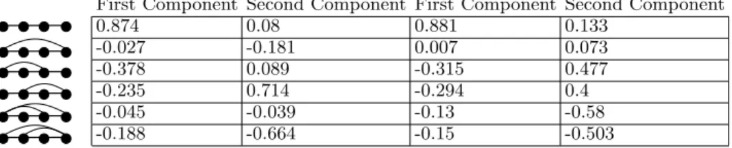
Chi&Yoga All States
First Component Second Component First Component Second Component
0.874 0.08 0.881 0.133 -0.027 -0.181 0.007 0.073 -0.378 0.089 -0.315 0.477 -0.235 0.714 -0.294 0.4 -0.045 -0.039 -0.13 -0.58 -0.188 -0.664 -0.15 -0.503
TABLE VI: Principal component scores obtained from PCA considering the subset data of Yoga and Chi meditators together (left) and and considering all data set (right).
[1] Albert R, Barabasi A-L, Statistical mechanics of complex networks.Rev. Mod. Phys.74,47 (2002).
[2] Boccaletti S, Latora V, Moreno Y, Chavez M, Hwang
D U Complex networks: structure and dynamics. Phys.
Rep.424,175 (2006).
[3] Newman M E JNetworks: An Introduction(Oxford
Uni-versity Press, 2010).
[4] Newman MEJ, The structure and function of complex
networks,SIAM Rev 45167-256 (2003)
[5] R. Milo, S. Shen-Orr, S. Itzkovitz, N. Kashtan, D.
Chklovskii, U. Alon, Network Motifs: Simple
Build-ing Blocks of Complex Networks, Science 298: 824-827
(2002)
[6] U. Alon, Network motifs: theory and experimental ap-proaches,Nature Reviews Genetics 8, 450-461 (2007). [7] R. Milo, S. Itzkovitz, N. Kashtan, R. Levitt, S.
Shen-Orr, I. Ayzenshtat, M. Sheffer, U. Alon, Superfamilies
of Evolved and Designed Networks, Science 303, 5663:
1538-1542 (2004)
[8] A. Masoudi-Nejad, F. Schreiber, Z.R.M. Kashani, Build-ing Blocks of Biological Networks: A Review on Major
Network Motif Discovery Algorithms.IET Systems
Biol-ogy 6, 5 (2012).
[9] Zhang J, Small M, Complex network from pseudoperiodic time series: topology versus dynamics.Phys. Rev. Lett. 96, 238701 (2006).
[10] Kyriakopoulos F, Thurner S, Directed network represen-tations of discrete dynamical maps, in Lecture Notes in Computer Science 4488, 625–632 (2007)
[11] Xu X, Zhang J, Small M Superfamily phenomena and motifs of networks induced from time series. Proc. Natl. Acad. Sci. USA105, 19601-19605 (2008).
[12] Donner R V, Zou Y, Donges J F, Marwan N, Kurths J Recurrence networks: a novel paradigm for nonlinear time series analysis.New J. Phys.12, 033025 (2010). [13] Donner R V, et al. The Geometry of Chaotic Dynamics
- A Complex Network Perspective.Eur. Phys. J. B 84,
653-672 (2011).
[14] L. Lacasa, B. Luque, F. Ballesteros, J. Luque and JC Nu˜no, From time series to complex networks: The visibil-ity graph,Proc. Natl. Acad. Sci. USA105, 13: 4972-4975 (2008).
[15] B. Luque, L. Lacasa, F. Ballesteros, J. Luque, Horizontal visibility graphs: Exact results for random time