HETEROGENEOUS EXPECTATIONS, FORECAST COMBINATION, AND ECONOMIC DYNAMICS
by
CHRISTOPHER G. GIBBS
A DISSERTATION
Presented to the Department of Economics and the Graduate School of the University of Oregon
in partial fulfillment of the requirements for the degree of
Doctor of Philosophy June 2013
DISSERTATION APPROVAL PAGE Student: Christopher G. Gibbs
Title: Heterogeneous Expectations, Forecast Combination, and Economic Dynamics This dissertation has been accepted and approved in partial fulfillment of the requirements for the Doctor of Philosophy degree in the Department of Economics by:
George Evans Chair
Jeremy Piger Core Member
Bruce McGough Core Member
Yue Fang Institutional Representative
and
Kimberly Andrews Espy Vice President for Research & Innovation/ Dean of the Graduate School
Original approval signatures are on file with the University of Oregon Graduate School.
c
DISSERTATION ABSTRACT Christopher G. Gibbs
Doctor of Philosophy Department of Economics June 2013
Title: Heterogeneous Expectations, Forecast Combination, and Economic Dynamics
This dissertation examines the forecast model selection problem in economics in both theoretical and empirical settings. The forecast model selection problem is that there often exists a menu of different suitable models to forecast the same economic variable of interest. The theoretical portion of this dissertation considers agents who face this problem in two distinct scenarios. The first scenario considers the case where agents possess a menu of different forecast techniques which includes rational expectations but where the selection of rational expectations is costly. The assumptions that are necessary to include rational expectations as a choice are characterized and the equilibrium dynamics of a model under the appropriate assumptions is studied and shown to exhibit chaotic dynamics. The second scenario considers agents who possess a menu of econometric forecast models and examines the equilibrium outcomes when agents combine the different forecasts using strategies suggested by the forecasting literature. The equilibrium outcomes under these forecasting assumptions are shown to exhibit time-varying volatility and endogenous structural breaks, which are common features of macroeconomic data.
The empirical portion of the dissertation proposes a new dynamic combination strategy for the forecast model selection problem to forecast inflation. The procedure builds on recent research on inflation persistence in the U.S. and on explanations for the efficacy of simple combination strategies, often referred to as the forecast combination puzzle. The new combination strategy is shown to forecast well in real-time out-of-sample forecasting exercises.
CURRICULUM VITAE
NAME OF AUTHOR: Christopher G. Gibbs
GRADUATE AND UNDERGRADUATE SCHOOLS ATTENDED: University of Oregon, Eugene, Oregon
Westminster College, Salt Lake City, Utah University of Utah, Salt Lake City, Utah DEGREES AWARDED:
Doctor of Philosophy in Economics, 2013, University of Oregon Master of Science in Economics, 2013, University of Oregon Bachelor of Science in Economics, 2008, Westminster College Bachelor of Science in Mathematics, 2008, Westminster College AREAS OF SPECIAL INTEREST:
Macroeconomics and time series econometrics GRANTS, AWARDS AND HONORS:
Invited Young Economist, 2011, Nobel Laureates Meetings, Lindau, Germany Best Ph.D. Field Paper, 2010, University of Oregon
Dale Underwood Scholarship, 2009, University of Oregon
First-year Econometrics Scholarship, 2009, University of Oregon Economics Faculty Appreciation Award, 2007, Westminster College
ACKNOWLEDGEMENTS
I wish to acknowledge my advisors George Evans and Bruce McGough for all the time and effort they have put into listening to my ideas and encouraging me along the way.
TABLE OF CONTENTS
Chapter Page
I. INTRODUCTION . . . 1
II. STRATEGIC EXPECTATIONS: FICTITIOUS PLAY IN A MODEL OF RATIONALLY HETEROGENEOUS EXPECTATIONS . . . . 4
Introduction . . . 4
The BH Model . . . 8
The Eductive Justification of the Rational Predictor . . . 12
Strategic Expectations . . . 21
Conclusion . . . 29
Supplementary Material and Proofs . . . 31
III. THE INFLATION GAP, FORECAST COMBINATION, AND THE FORECAST COMBINATION PUZZLE . . . 37
Introduction . . . 37
Predicting Forecast Errors . . . 40
Candidate Forecasts and Data . . . 43
Real-Time Forecasts . . . 50
Forecast Tournament . . . 55
Conclusion . . . 58
Chapter Page
IV. FORECAST COMBINATION IN THE MACROECONOMY . . . 71
Introduction . . . 71
A General Framework . . . 75
Exogenous and Endogenous Selection of Weights . . . 81
Learning FCEs . . . 100
Learning in Real Time . . . 108
Forecast Combination Equilibria and Actual Forecasting . . . 113
Conclusion . . . 116
Supplementary Materials and Proofs . . . 118
V. CONCLUSION . . . 125
LIST OF FIGURES
Figure Page
1. Bifurcation diagrams with respect to β . . . 34
2. Bifurcation diagrams with respect to γ . . . 35
3. The forecast errors of fictitious play learning . . . 36
4. PCE inflation, the PIGC forecast of PCE, the equal weights forecast of PCE, and time-varying weights of PIGC . . . 59
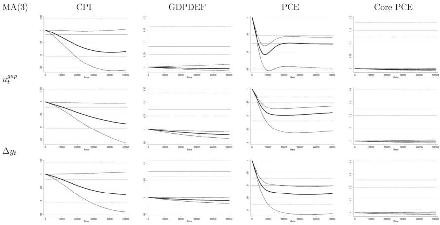
5. Mean, minimum, and maximum relative RMSFE of PIGC . . . 60
6. Mean, minimum, and maximum relative RMSFE of PIGC . . . 61
7. Bifurcation on the center manifold of the T-map . . . 92
8. A plot of the OWFCE forecasts . . . 94
9. A plot of the OWFCE forecasts and the REE forecast . . . 95
10. Plots of the ROWFCE forecasts . . . 98
11. E-stability of the OWFCEs and ROWFCEs . . . 106
12. E-stability of the fundamental FCE under OWC . . . 107
13. Time-varying volatility with vt∼N(0,1) . . . 110
14. Time-varying volatility with vt∼N(0,2) . . . 111
LIST OF TABLES
Table Page
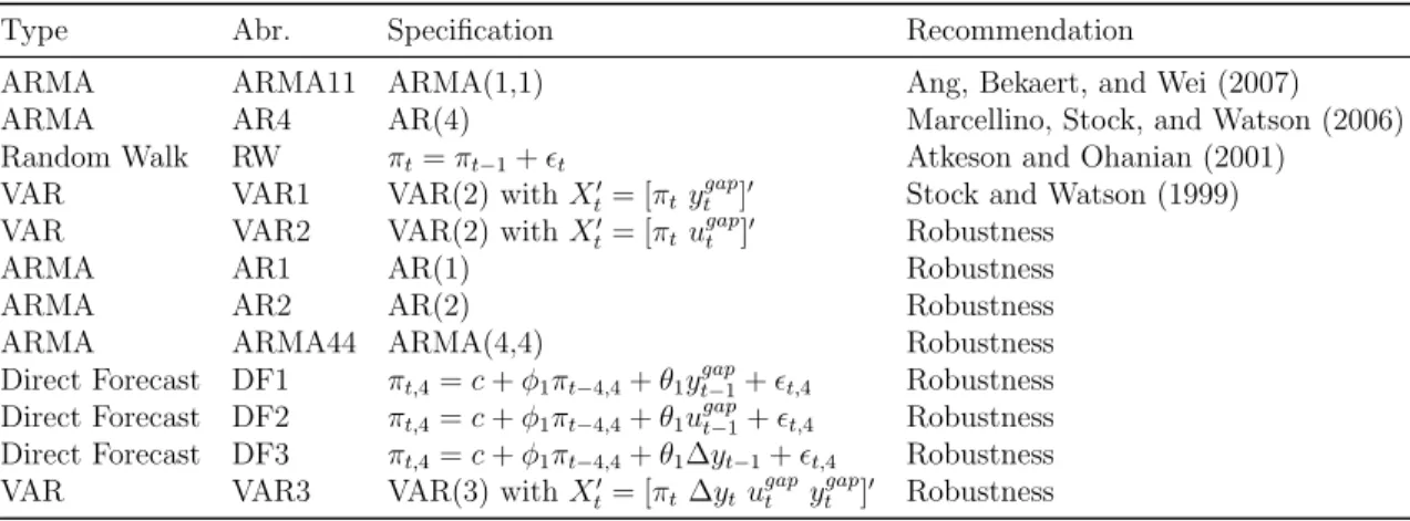
1. Candidate forecast models . . . 46
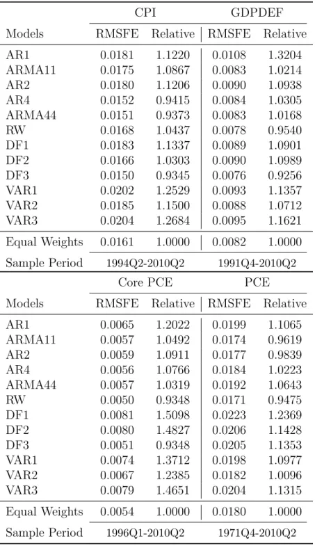
2. RMSFE for the candidate forecasts of inflation compared to an equal weights combined forecast . . . 48
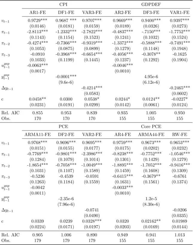
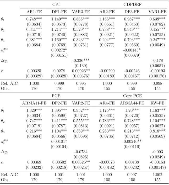
3. Parameter estimates for the model of forecast error dynamics . . . 62
4. Parameter estimates for the model of forecast error dynamics . . . 63
5. Intercept corrected forecasts of inflation . . . 64
6. Data subsets for implementation of PIGC. Relative RMSFE of PIGC . 65 7. Forecast tournament results for Core PCE . . . 66
8. Forecast tournament results for CPI . . . 67
9. Forecast tournament results for GDP Deflator . . . 68
10. Forecast tournament results for PCE . . . 69
11. The cumulative tournament ranking of each combination method . . . 70
12. Tabulated results for the FCEs . . . 101
CHAPTER I INTRODUCTION
This dissertation consist of three stand-alone pieces of research that are each variations on a common theme: the selection and combination of forecasts. The research topic covers a broad literature in economics that includes empirical and theoretical research. This dissertation makes contributions to both literatures and in many instances bridges the divide between dynamic macroeconomic theory and the applied practice of forecasting.
The first chapter considers an expectation formation problem in the dynamic macroeconomic theory literature. The literature considers deviations to standard equilibrium outcomes that may arise when individual agents face a cost to forming optimal or rational expectations. The goal of the literature is to endogenize the rationality of the agents by explicitly modeling the fact that information and complex computations are costly. The seminal paper in this literature is Brock and Hommes (1997) who posit a model where agents possess a menu of ways to form expectations that each have different implementation costs. Brock and Hommes show that when heterogeneous agents are allowed to endogenously choose between costly rational expectations or free naive expectations that the market outcomes can exhibit chaotic dynamics.
However, the results obtained by Brock and Hommes raise questions about the validity of assuming rational expectations, even for a cost, in a model where agents can explicitly choose non-rational expectations. The problem is that rational expectations requires agents to coordinate independently on a unique expectation to hold and the traditional assumptions that underlie the coordination may not be satisfied in
the presence of non-rational agents. I study the assumptions underpinning rational expectations in the Brock and Hommes model to characterize the conditions under which coordination is a strategic or rationalizable outcome of the model using the eductive approach to studying expectations.
The eductive justification of rational expectations is that rational expectations directly follows from assuming the common knowledge of rationality, meaning that each agent is rational and knows that all other agents are rational and so on. I show that conditions under which coordination is found to not be a consequence of the common knowledge of rationality coincide with the conditions for chaotic dynamics in the Brock and Hommes model. I then propose an extension to their model to explore the impacts of coordination failures on equilibrium dynamics.
The second chapter considers multiple ways to form expectations in an applied forecasting problem. In the practice of forecasting there often exists a plethora of suitable ways to forecast the same macroeconomic variable of interest. It is also common to find that among the suitable methods the efficiency or accuracy of the different forecasts varies greatly over time. The instability and uncertainty that surrounds many forecast methods has prompted practitioners to consider ways to combine the many reasonable forecasts into one. A natural question that arises when combining forecasts is whether or not there exist an optimal way to combine the forecasts.
The pursuit of this question has led to an empirical puzzle. The best forecast combination procedure in practice is often a simple average of forecasts. The result is consistently obtained despite the fact that the theoretically optimal weights for a combination strategy based on the properties of the data under study often deviate substantially from the equal weights implied by averaging. The result is known as
the forecast combination puzzle. In this chapter I propose a new dynamic forecasting procedure for inflation that can robustly beat the simple average of forecasts by exploiting a hypothesis for why the forecast combination puzzles exists and new empirical finding from the inflation literature. The procedure is shown to create robust and efficient forecasts on four different measures of inflation in real-time out-of-sample forecasts.
The third chapter returns to dynamic macroeconomic theory and considers the effects of the widespread use of forecast combination strategies, like those discussed in Chapter 2, on the macroeconomy. I proposes an equilibrium concept where homogeneous economic agents possess a menu of ways to forecast an endogenous variable. The agents combine the forecasts using a forecast combination strategy to create a single forecast of the endogenous variable of interest to make dynamic decisions in the model.
The combined forecasts or expectations studied in the model are self-referential, which allows for the exploration of possible unanticipated endogenous effects of employing common forecasting strategies that cannot be captured in forecasting exercises like those undertaken in Chapter 2. Forecast combination strategies are largely atheortic with respect to economic theory and their justification lies solely on their ability to perform well in “pseudo” out-of-sample forecasting exercises. Results and conclusions based on these types of studies may lack external validity because they do not capture the self-referentiality that exists in the macroeconomy, where forecasts lead to changes in agent behavior that ultimately dictates the accuracy of the forecast. I show that the consideration of self-referentiality of combined forecasts can have significant implications for macroeconomic dynamics and model predictions.
CHAPTER II
STRATEGIC EXPECTATIONS: FICTITIOUS PLAY IN A MODEL OF RATIONALLY HETEROGENEOUS EXPECTATIONS
Introduction
The dominant paradigm in dynamic macroeconomics is to model homogeneous forward-looking agents who possess rational expectations (RE). The calculation of RE is intuitively a costly process due to the amount of information and number of computations an economic agent must undertake to obtain a proper expectation. This cost implies that under certain circumstances it may be utility or profit maximizing to forgo calculating a rational expectation.
A model of rationally heterogeneous expectations (RHE) explicitly captures this scenario by assuming that agents possess a menu of ways to form expectations about the future value of endogenous state variables. The menu of ways to form expectations, known as predictor rules, includes rational expectations along with other less sophisticated rules. The predictor rules have different costs to implement based on the information and cognitive power necessary to calculate an expectation. The agents evaluate the predictors based on a fitness criterion that incorporates the costs of using each rule. The agents endogenously select among the predictor rules over time as the relative fitness of each rule changes.
The seminal paper in this literature is Brock and Hommes (1997), “A rational route to randomness” (hereafter referred to as BH).1 BH models heterogeneous agents 1The RHE genesis is from the related idea of calculation equilibria proposed by Evans and Ramey (1992 and 1998) who studied agents who pay a cost to incrementally improve an expectations. They found that under certain circumstance it is optimal for the agents to not select fully rational expectations.
in a cobweb model who possess an explicit choice of rational expectations for a cost or naive expectations for free. The agents select among the two predictor rules based on the past observed net profits of each predictor. The model results in an equilibrium price process that BH calls Adaptively Rational Equilibrium Dynamics (ARED), which under certain conditions is shown to converge to a strange attractor and generates chaotic price dynamics.
The necessary condition identified in the BH model for chaotic dynamics is that the relative slopes of supply and demand must be greater than one. This condition exactly coincides with the necessary and sufficient condition identified by Guesnerie (1992) for the rational expectations equilibrium of the cobweb model to lack strong rationality. The lack of strong rationality means that individual agents, who possess only the common knowledge of rationality and full information about the parameters of the model, cannot coordinate on a unique rational expectation to hold.2 The coinciding conditions raise the question of whether the outcomes of the model are the plausible result of individually rational firms competing in a market.
This is an interesting question because of the volume of research that has adopted the RHE modeling structure. The basic RHE framework has been studied in asset pricing models as in Brock and Hommes (1998), Gaunersdorfer (2000), and Brock, Hommes, and Woo (2009); the New Keynesian model as in Branch and McGough (2010); and in further detail in the cobweb model in works such as Brock, Dindo, and Hommes (2006) and Branch and McGough (2004 and 2008). The common finding is that heterogeneous agents with an explicit choice to hold costly rational expectations or free naive expectations can lead to exotic or chaotic dynamics. In addition, there exists a large literature that considers predictor rule selection without including the 2The existence of strong rationality is referred to as the eductive justification for rational expectations.
choice of a rational predictor such as in Chiarella and He (2003) and Branch and Evans (2006 and 2007). The possible implausibility of the rational predictor based on the lack of strong rationality provides justification for studying models that omit rational expectations.
I employ the eductive learning approach of Guesnerie (1992) to study the strategic motivation of predictor selection and of the rational predictor in the BH model. The term strategic is used to connote that the model’s predictions are the unique outcomes resulting from individually rational agents competing in a game. I first establish that predictor selection requires a coordination assumption beyond standard RE in order to be well-defined. I then show that the rational expectations predictor, given this coordination assumption for selection, is not a strategic outcome for a broad range of the relevant parameter space. The two results imply that ARED is not justified as an outcome of rationally heterogeneous agents competing in a market, but is the result of strong implicit assumptions that coordinate agents’ actions.3
The justification that BH is not a strategic outcome is based on analyzing an agent’s predictor choice and expectation formation from a game theoretic perspective. Therefore, I propose to use another concept from game theory, fictitious play, to add a minimal amount of plausible strategic interaction into the BH framework to explore the implications of a deviation from the standard RHE assumptions. I call this new equilibrium concept Fictitious Play Equilibrium Dynamics (FPED).
Fictitious play is an adaptive learning approach to playing a game with an unknown and possibly changing opponent. Fictitious play has agents form an empirical distribution of the likely play of their competitors based on the history of 3Hommes and Wagener (2010) show that eductive stability of the underlying cobweb model studied in BH does not imply evolutionary stability when heterogeneous agents select among different predictor rules. But, the eductive stability of the BH framework itself and rational expectations is
past play. The agents then choose their strategy as a best response to the empirical distribution. The concept was originally proposed by Brown (1951) as a plausible way agents could compute and coordinate on a Nash equilibrium. More recent treatments and variations of the approach are found in Fudenberg and Kreps (1993), Young (2001), and Waters (2009).4
There are a number of advantages to adopting fictitious play as an expectation and coordination device for heterogeneous agents in the BH framework. The first is that fictitious play makes agents’ predictor selection explicitly strategic by requiring agents to best respond to the expected contemporaneous actions of their competition. This feature is inherent to the BH model, but as Branch and McGough (2010) point out, has not been addressed in the literature. The second is that fictitious play is a forward-looking selection mechanism. The agents try to anticipate the other market participants’ expectations based on past observations. This builds on the work of Brock, Dindo, and Hommes (2006) (hereafter Brock et al.), who study forward-looking ARED under rational expectations by adding a learning component to their model. The third is that fictitious play provides a plausible way agents could actually form strategically motivated expectations, which may provide insight into explaining the experimental results of “learning to forecast” studies such as Hommes et al. (2005 and 2007) and Hommes (2011). Finally, fictitious play has stable equilibrium dynamics in the cobweb model if agents use the process to pick production quantities rather than predictor rules as demonstrated by Thorlund-Petersen (1990).5 In addition, Branch (2002) shows that the inclusion of a free learning-based predictor rule results 4Waters (2009) analyzes a fictitious play like mechanism for selecting predictor rules in the cobweb model. The paper, however, does not use it to address the strategic issue of predictor rule selection. 5The fictitious play stability results demonstrated in Thorlund-Petersen (1990) is in a multi-player Cournot model. The Cournot model is the finite player version of the cobweb model.
in stable equilibrium dynamics. The stability of the dynamics, when learning is present, suggests that the implicit coordination assumptions of the rational predictor may be the main driver of the dynamics. However, I show this is not the case.
The equilibrium dynamics under fictitious play replicate many of the key features of ARED in a forward-looking model with either heterogeneous or homogeneous agents. The addition of fictitious play makes the firms’ beliefs a state variable of the economy. The market structure is such that there is an incentive to deviate from the predictor rule when a firm believes that the majority of market participants will select it. These incentives result in a perpetual miscoordination between beliefs and outcomes that helps to drive the equilibrium price dynamics.
The remainder of the paper proceeds as follows. Section 2 introduces the BH model and discusses the strategic decision the agents face. Section 3 explores the strategic justification of the BH model. Section 4 introduces Fictitious Play Equilibrium Dynamics and demonstrates its properties. Section 5 concludes.
The BH Model
The model of BH is a linear cobweb model that describes the price dynamics of a competitive market with a non-storable good that has a one-period production lag.6 The model features a continuum of identical firms who select among a fixed menu of predictor rules to forecast price in order to choose a profit-maximizing quantity of goods to supply to the market. The production decision is made at time t and the goods are produced and sold at timet+ 1. The market demand at timet+ 1 is
D(pt+1) =A−Bpt+1; A >0, B >0. (2.1) 6The notation adopted follows Brock et al. (2006)
The firms supply to the market based on their expectation of price at time t + 1, which is denoted as pe
j,t+1, where j indicates the jth firm’s expectation. The firm’s expectation is used to produce a profit-maximizing quantity according to
S(pej,t+1) = argmaxqj,t{p e
j,t+1qj,t−c(qj,t)}. (2.2)
The firms each face an identical cost function,
c(qj,t) = q2
j,t
2b, b >0, (2.3)
which results in a unique profit-maximizing quantity of goods to supply to the market, given an expectation of price:
S(pej,t+1) =bpej,t+1. (2.4)
The firms choose between two predictor rules to form a forecast of price in each period t. The firms can choose the rational predictor, denoted p1t+1,e = pt+1,
for an explicit cost C ≥ 0 or a naive predictor, denoted p2t+1,e = pt, for free. The
cost is imposed to represent the extra computational power and information that is necessary to calculate a rational expectation. The fraction of firms that choose the rational predictor is denoted n1
t and the fraction of that choose the naive predictor is
denoted n2t. Given the fractions of firms, the market clearing condition is
D(pt+1) = n1tS(p 1,e t+1) +n 2 tS(p 2,e t+1). (2.5)
Strategic Decisions
There are potentially two strategic decisions that firms face each period. The firms must select a predictor rule, and contingent on the selection of the rational predictor, they must select a rational expectation. The choice of a predictor is strategic because of the explicit cost of choosing the rational predictor. The cost creates a trade-off between investing resources to calculate a correct forecast and lost profits that may occur due to forecast errors. The size of the forecast errors depend on market volatility, which depends on agents’ predictor choices. The rational predictor is always a strategic expectation in that it must take into account both the naive and rational forecasts of the other firms in order to determine the correct expectation.
The BH framework introduces a behavioral assumption that removes the strategic element from the predictor selection decision. The firms ignore the strategic aspect of selecting a predictor rule by being backward-looking. The firms choose predictor rules by comparing the past realized profits of each rule, net the cost of implementation. The past profit of each predictor is given by
πti =π(pt, p i,e t ) = b 2p i,e t (2pt−p i,e t )−Ci (2.6)
for i = 1,2 and is considered public information. The past profits are called the fitness measure.
The fraction of firms that choose each predictor is determined by the fitness measure and a discrete-choice econometric model:
nit = e βUi t P2 i=1eβU i t , (2.7)
where Ui
t, the fitness measure, is Ut1 = πt1 −C or Ut2 = πt2. The parameter β is
called the intensity of choice parameter and it governs the relative size of the fraction of firms that choose each rule based on the realization of the fitness measure. The intensity of choice parameter is a proxy for the firms’ uncertainty over their choices. If β is large, then more firms use the rule with highest past profit. BH closes the model by definingmt =n1t−n2t and substituting in the predictor rules into the market
clearing condition (2.5) to yield the following system of equations
A−Bpt+1 = b 2(pt+1(1 +mt) +pt(1−mt) (2.8) mt+1 = Tanh[ β 2( b 2(pt+1−pt) 2− C)]. (2.9)
BH defines equations (2.8) and (2.9) as Adaptively Rational Equilibrium Dynamics (ARED).
The ARED system has a unique steady-state
E∗ = ( A
B+b,Tanh[− βC
2 ]) (2.10)
and possesses the following stability properties:
Result 1: (BH Theorem 3.4) Assume that the slopes of supply and demand satisfy
b/B >1
i. When the cost of the rational predictor is C = 0, the steady-state E = (¯p,0) is globally stable.
ii. When the cost of the rational predictor is C > 0, then there exists a critical value β1 such that for 0 ≤β < β1 the steady state is globally stable, while for
β > β1 the steady state is an unstable saddle path with eigenvalues 0 and
λ(β) =− b(1−m
∗ (β)) 2B+b(1 +m∗(β)).
At the critical valueβ1 the steady state value m∗(β1) = −B/b
iii. When the steady state is unstable, there exists a locally unique period 2 orbit
{(ˆp,mˆ),(−p,ˆ mˆ)} with ˆm =−B/b. There exists aβ2 > β1 such that the period cycle is stable for β1 < β < β2.
Result 2: (BH Theorem 3.2) For β = +∞, even when the market is locally unstable (i.e. b/B > 1) and when the cost of the rational predictor is C > 0, the system always converges to the saddle point equilibrium steady state E∗.
Furthermore, if β is set to a significantly large value, C > 0, and b/B > 1, then ARED may exhibit chaotic price dynamics. Examples of the dynamics are given in Section 4.
The Eductive Justification of the Rational Predictor
The rational predictor is inherently a strategic calculation where rational firms must anticipate the combined effect of all agents’ expectations on the market price to determine a correct expectation to hold. The strategic justification of this calculation is to determine whether the agents are capable of independently coordinating on the RE price possessing only the common knowledge of rationality (CK):
Common Knowledge of Rationality: The individual knowledge by a rational firm of the structure of the economy and that all other firms are rational and know the
structure of the economy and that all firms know that the other firms know and so on.
A rational expectation is strategically or eductively justified if the agents, given the stated assumptions, can coordinate on a unique expectation to hold through iterated deletion of strictly dominated strategies. In what follows, I present the basic results from Guesnerie’s (1992) analysis of the cobweb model without predictor rule selection to motivate and demonstrate the tools necessary to analyze the more complicated case.
The basic cobweb model is composed of a linear demand and supply functions given by equations (2.1) and (2.4). The unique rational expectations equilibrium (REE) of the model is
¯
p= A
B+b. (2.11)
The REE is strategically or eductively justified if the following definition holds:
Strongly Rational: A rational expectation is strongly rational if it is the unique rationalizable expectation for firms to hold assuming the common knowledge of rationality.
The strong rationality of an expectation is determined by analyzing the strategic choices of agents as a one period normal-form game. The cobweb model can be formulated as a game with a continuum of players on the unit interval,J = [0,1]. The strategy set of the players is all feasible pricesP = [0, A/B] such that an individual’s price expectation is pe ∈ P. The aggregate expected price in the market is R
pe jdj,
which given equation (2.4) results in a market supply of bR pe
price p =D−1(bR pe
jdj). The jth firm’s best response in this game is to pick pe such
that pe=p.
The agents choose a best response using iterated deletion of strictly dominated strategies. Given the common knowledge of rationality, it follows that each firm only chooses strategies that are best responses to the possible profile of strategies other rational firms would actually play. Therefore, there may exist a subset of strategies that are never played because they are never best responses. If the firms eliminate these strategies, then they have a smaller feasible strategy setP1 ⊂P from which to choose. The smaller strategy setP1, however, can be put through the same deduction and the firms may again be able to discard strategies to arrive at P2 ⊂ P1 ⊂ P. If firms continue this line of reasoning, it may be possible to reduce the strategy set to
P∞=pe, which implies that each firm will conclude there is only one price expectation a rational firm would choose. For the cobweb model, if P∞ = ¯p, it is said that ¯p is strongly rational.
Result 3: Guesnerie (1992): Proposition 1 - Given equations (2.1) and (2.4), i) if b/B <1, then REE of the cobweb model is strongly rational. ii) If b/B ≥1, then the REE of the cobweb model is not strongly rational and the set of rationalizable prices is P.
Therefore, in the basic cobweb, the REE is not a consequence of strategic interaction when b/B≥1.7
7The term rationalizable means that a strategy is not strictly dominated by another feasible strategy.
The Common Prior
The assumption necessary for coordination of rational expectation in the absence of strong rationality is that firms hold model consistent beliefs or beliefs that are in line with ”the relevant economic theory,” as stated in Muth (1961). This belief is called by Aumann and Dreze (2008) the common prior belief (CP):
Common Prior Belief: The strategy choices of different types of agents are common knowledge.
The CP is a coordinating assumption akin to the law iterated expectations for heterogeneous agents, where firm j’s expectation of firm k’s expectation of price is EjEk[p] = Ej[p] for j 6= k.8 If agents possess the common knowledge of rationality and the common prior belief, they can select the REE price from the set of rationalizable prices with the expectation that the other firms will make the same choice.
Strategic Interaction in ARED
The cobweb game with predictor selection is more complicated. The firms in the expanded game have two choices: they must select a predictor and then choose an expectation of price. The predictor choice can be thought of as the agents choosing a type. If agents choose the rational predictor, then they play the cobweb game as described in the previous section. If they choose the naive predictor, then they abandon strategy and choose last period’s price. The CP assumption in this context 8The idea of an analog to the law of iterated expectations for heterogeneous agents is also explored in Branch and McGough (2009) in the context of the New Keynesian model.
is not sufficient to motivate predictor rule choices or the rational predictor because the agents cannot always deduce the distribution of player types.
To illustrate the issue, suppose that the firms who select the rational predictor are endowed with CK and CP, where CP imparts the knowledge of each type’s strategy, but does not include information about n1t or n2t, the fraction of types. Knowledge of the fraction of firms that choose each rule is necessary to calculate a rational expectation and to choose a predictor rule. Under certain conditions, without knowledge of the fractions, the firms cannot deduce a unique predictor to select. Each predictor or firm type is rationalizable given the other agents’ potential actions. To formalize the argument, let the fraction of firms who choose the rational predictor be
n, the fraction of naive firms be 1−n, and let the naive predictor forecast be denoted
p−1.
Theorem 1: Suppose that the firms are endowed with CK and CP. The firms can deduce that i. if |p¯−p−1| ≤ BB+b q 2C b , then n = 0 and p 2,e =p
−1 is the unique rationalizable predictor choice.
ii. if|p¯−p−1| ≥ q
2C
b , thenn= 1 andp
1,e =pis the unique rationalizable predictor
choice. iii. if |p¯− p−1| ∈ (BB+b q 2C b , q 2C b ), then both p 2,e = p −1 and p1,e = p are rationalizable.
Proof: The firms are profit maximizers and will choose the predictor rule with the highest profit. The rational predictor under ARED assuming CK and CP is
p= A−(1−n)bp−1
B+bn . (2.12)
Equating profits of the predictors for an unspecifiedn results in
π1 = π2
b
2p
2−C = b
2p−1(2p−p−1).
Solving the equation the for p−1 and substituting in (2.12) yields
p1−p¯=± B+bn B+b r 2C b , where ¯p=A/(B+b). (i) If |p¯−p−1| ≤ BB+b q 2C
b , then the rational predictor is never
more profitable than being naive, therefore all agents choose to be naive and n = 0. (ii) If |p¯−p−1| ≥
q 2C
b , then the naive predictor is never more profitable than the
rational predictor and all agents will choosen = 1. (iii) If|p¯−p−1| ∈(BB+b q 2C b , q 2C b ),
then there exists n ∈ (0,1) such that π1 = π2. Therefore, the rational and naive predictors are each rationalizable. Q.E.D.
The agents are unable to determine the contemporaneous strategy choices of the other firms for a range of feasible prices because if the strategies are chosen in exactly the right proportions, then a firm is indifferent between the rational or naive predictors. Anyn ∈[0,1] could result in the model because there is no way to coordinate which firms choose the rational predictor and which firms chooses the naive predictor to
enforce the correct fraction given a realization ofp−1in the relevant range.9 Therefore, the standard assumptions invoked when using rational expectations are not sufficient to justify the firms’ deduction ofn or the realization of n as a market outcome when there exists rationally heterogeneous expectations.10
Rationally heterogeneous expectations requires an additional assumption to justify the knowledge of n for the range of feasible prices where there exists heterogeneous predictor choices. We define this assumption as thenon-rational agent common prior belief (NACP)
Non-rational Agent Common Prior: The fraction of firms who choose the rational predictor is n and the selection of the rational predictor imparts common knowledge among the rational firms of n.
The NACP assumption is similar to the notion of a Correlated equilibrium, where firms are told a strategy to choose and it is rational for a firm to choose that strategy given all players follow their instructions.11 The NACP assumption is invoked in the BH model by assuming it is common knowledge that predictor selection is based on past profit and knowledge of the discrete choice rule given by equation (2.7) that governs the precise fraction of firms that choose each rule.
The knowledge of n is necessary to form a rational expectation, which implies that NACP is a necessary condition to form a rational expectation in ARED. Thus, 9The third case is an example of a mixed strategy equilibrium. However, the playing of mixed strategies is not permitted.
10Note that this is a stronger result than that of strong rationality because it holds for allb/B. 11See Aumann and Dreze (2008) for more information on the relationship between Correlated equilibria and RE.
the next question is to determine whether CK and NACP are the only necessary conditions to make the rational predictor a strategic outcome of the model.
Theorem 2: Given CK and NACP, the rational predictor of ARED is i) strongly rational if nb/B < 1. ii) The rational predictor is not strongly rational if nb/B ≥1 and the set of rationalizable prices is P0 = [0,(A−b(1−n)p−1)/B].
Proof: The agents who choose the RE predictor possess CK and NACP, which implies they know market clearing is given by
A−Bp=nbpe+ (1−n)bp−1
Market clearing can be rewritten as
p=µ0+µ1pe,
where µ0 = (A−b(1−n)p−1)/B and µ1 = nb/B. The agents possess CK, so the result is obtained by applying Result 3. Q.E.D.
The intuition for theorem 2 is that the rational agents know at a minimum (1−n)bp−1 of goods will be supplied to the market. This implies that the highest price the market will obtain is pH = D−1((1 −n)bp−1), which results in an initial feasible strategy set of P0 = [0, pH]. The agents can perform iterated deletion of strictly dominated strategies by exploring whether pH is ever a best response. If the
agents that choose the rational predictor expect pH, then the price next period is p1 = D−1(nbpH + (1 −n)bp−1). If nb/B < 1, then 0 < p1 < pH and all pe < p1,
such that pe ∈ P
0, are revealed to never be best responses. This results in a smaller feasible set P1 = [p1, pH] of possible best responses. The agents can continue the deduction by evaluating whether p1 is a best response. The firms will find that this again leads to the elimination of more strategies. If the deduction is continued it will eventually converge to the rational expectation price forecast. If however nb/B ≥1, then p1 ≤0 and no prices are eliminated for being a best response. The entire set P0 is rationalizable.
The conditions of Theorem 2 for strong rationality are less restrictive than in the standard case presented in Result 3. For n < 1, the firms can coordinate on a rational expectation for values of b/B where coordination is not justified in the basic cobweb framework. This has a nice economic intuition because as n increases, the number of agents whose forecasts are known with certainty decreases. The more uncertainty that enters the market, the harder the agents find it to coordinate on a single rational expectation. However, this result does not necessarily imply that the rational predictor is strategically justified for a range of b/B that greatly exceeds Result 3 because n is dynamic in ARED. If b/B > 1, then the instability of the price dynamics will cause n to fluctuate between zero and one. The fluctuations may lead to periods where coordination is not strategically justified. The likelihood of unjustified coordination rises with the instability of the dynamics and with the likelihood of chaotic dynamics.
Theorems 1 and 2 show that CK, CP, and NACP are the implicit coordination assumptions that are necessary to coordinate actions in ARED. The ARED framework is not well defined under only the CK assumption by Theorem 1, and the rational predictor is in general not strategically justified under CK and NACP by Theorem 2 in the relevant parameter space. Hence, there is in general no strategic justification for
the interesting ARED outcomes in the current modeling framework. The dynamics are not the result of rationally heterogeneous firms competing in a market, but they are the manifestation of strong coordinating assumptions. This implies that the inclusion a rational predictor rule is no more justified than the inclusion of a heuristic, econometric, or boundedly rational rules on the menu of predictor choices to coordinate agent behavior.
Strategic Expectations
The inclusion of the rational predictor, however, is a natural modeling choice in dynamic macroeconomics. Therefore, in this section I propose an extension to ARED that adds a strategic element to the model while retaining as much of the original structure as possible. The dynamic properties of the extension are characterized and compared to ARED.
The CK and CP assumptions are standard in macroeconomics and are retained in what follows. The NACP is non-standard and I focus my attention on adding strategic interactions to model this assumption. I modify the NACP assumption employed in BH by assuming that firms engage in fictitious play. The firms construct an empirical estimate of the distribution of predictor choices in an average period to create an expectation of the contemporaneous predictor rule choices that will take place in the current period. The firms then choose a predictor rules as a best response to this expectation.
Fictitious play is added to the existing framework by assuming firms estimate the difference in the fraction of firms who choose the rational and naive predictors. The firms use the estimate to pick a best response and if they choose the rational predictor, they use the estimate ofmt along with CK and CP to form an expectation.
The firms estimatemt using a simple learning rule
ζt+1 =ζt+γ(mt−ζt), (2.13)
where ζt+1 is the estimated difference in the fraction of firms that choose each predictor and 0 < γ ≤ 1 is the gain parameter that governs the weight placed on new observations.12 The firms use the estimate to calculate the expected profitability of the two predictor rules and the predictor with the highest expected profit is chosen. This best-response assumption requires the firms to be forward-looking, which introduces a simultaneity issue into the BH framework when the cost of the rational predictor is positive. The firm must know the rational forecast in order to know whether it is profitable to pay the cost and choose the rational predictor. This is a known issue of dynamic predictor selection models and is addressed in Brock et al. (2006), who investigate forward-looking ARED under rational expectations. I employ a similar framework to the one they developed to overcome the simultaneity issue.
The Expert Manager
Brock et al. (2006) posits the existence of a single expert manager who has the ability to form rational expectations and charges the firms a fee for her service. I modify this concept and assume that there exists a continuum of expert managers on the unit interval that have structural knowledge about the economy equivalent to the CK and CP assumptions. An expert manager can be hired by the firm for the fee C ≥ 0 in order to calculate an expert prediction. An expert manager can only provide services to one firm each period. There is perfect competition among 12The gain parameter is a common feature of learning models in macroeconomics. For a more in depth discussions see Evans and Honkapohja (2001).
the managers and any firm can hire any manager, which results in a uniform fee that is equal to the expert managers’ marginal cost of producing a prediction C≥0. The expert managers possess CK and CP which implies that their price expectations are coordinated given a shared belief of ζt, the fraction of firms believed to hire an
expert manager in each period. The fraction of firms that hire an expert manager and the expected net profits of doing so are public information.13 The information can be thought of as provided by a government agency that monitors the market. The fraction of firms that hire an expert manager in a given period is determined by the discrete-choice random-utility framework of the original BH model given by equation (2.7).
The expert managers use the belief ζt, CK, and CP to produce the following
price prediction:
p1M,t,e +1 = 2A−bpt(1−ζt) 2B+b(1 +ζt)
. (2.14)
An expert manager’s prediction is identical to the rational predictor of ARED, except that mt is replaced with ζt. An expert manager is acting strategically in using ζt to
form a forecast by attempting to predict the contemporaneous strategy choices of the other firms and the effect those choices will have on realized profits. The expert managers’ prediction is used to calculate the expected profits of paying for their 13An additional assumption is made in Brock et al. (2006) that the fee is unknown to firms to prevent the firms from reverse engineering the price forecast from the advertised expected net profit. I omit this assumption because the reverse engineering violates the spirit of the cost associated with rational expectations. A firm that reverse engineers the price would have to pay the same cost as hiring a manger to do so.
service or remaining naive using the following equations: π1t+1,e = b 2( 2A−bpt(1−ζt) 2B +b(1 +ζt) )2−C (2.15) π2t+1,e = b 2pt( 2A−bpt(1−ζt) 2B+b(1 +ζt) −pt). (2.16)
The resulting expected net profits are advertised to the firms and used as fitness measure to make a hiring decision.
As acknowledged in Brock et al. (2006), the expert manager is a limited description of market behavior. But, given the difficulties that exist with modeling heterogeneous agents, it is an interesting theoretical benchmark to consider and a necessary assumption in order to make direct comparisons to past work.
Fictitious Play Equilibrium Dynamics
The expert manager’s profit advertisements, the predictor PM,t1,e+1, the discrete choice model, and the learning rule together form Fictitious Play Equilibrium Dynamics (FPED): A−Bpt+1 = b 2( 2A−bpt(1−ζt) 2B+b(1 +ζt) (1 +mt) +pt(1−mt)) (2.17) ζt+1 = ζt+γ(mt−ζt) (2.18) mt = Tanh[ β 2( b 2( 2A−bpt(1−ζt) 2B +b(1 +ζt) −pt)2−C)]. (2.19)
FPED has two state variables pt and ζt. The introduction of fictitious play makes
The switch from outcomes to beliefs only introduces subtle changes to the dynamics properties of the market for small values of the intensity of choice parameter. Fictitious Play Equilibrium Dynamics retains the same unique fixed point as ARED
E∗ = (p∗, ζ∗) = (¯p,Tanh[−βC
2 ]) (2.20)
and it possesses the following stability properties.
Theorem 3: Assume that the slopes of supply and demand satisfy b/B > 1 and 0< γ≤1
i. When the cost of the rational predictor is C = 0, the steady-state E = (¯p,0) is locally stable.
ii. When the cost of the rational predictor is C > 0, then there exists a critical value β1 such that for 0 ≤ β < β1 the steady state is locally stable, while for
β > β1 the steady state is an unstable saddle path with eigenvalues 1−γ and
λ(β) = −b(B+bζ
∗(β) + (b+B)Tanh(βC/2))
B(b+ 2B+bζ∗(β)) . At the critical valueβ1 the steady-state value ζ∗(β1) =−B/b
iii. When the steady state is unstable, there exists a locally unique period 2 orbit
{(ˆp,ζˆ),(−p,ˆ ζˆ)} with ˆζ = −B/b. There exists a β2 > β1 such that the period cycle is stable for β1 < β < β2.
The proof appears in the appendix. Result 1 and Theorem 3 reveal that the FPED has similar dynamics to ARED locally and for small values of β. However, The two systems diverge globally and for large values ofβ, whenβapproaches positive infinity.
Theorem 4: Assume that the slopes of supply and demand satisfyb/B >1,C >0 and β = +∞, then E = (¯p,−1) is an unstable saddle path if 0< γ <1 and globally stable if γ = 1.
Theorem 4 illustrates the effect that strategic interaction has on coordination. When 0< γ <1, the firms have uncertainty over the contemporaneous choices of the other firms in the market, which is grounded in past observed behavior. The firms observe heterogeneous predictor rule selection between periods and they posit that there may exist heterogeneous predictor rule selection within each period. The best response of the firms is to incorporate this uncertainty into their expectations. The uncertainty drives a wedge between beliefs and actual actions that can never be overcome. It is only when the firms discard information (i.e. γ = 1) that the uncertainty is removed and coordination is achieved.14 The same intuition of perpetual miscoordination of belief and actual actions taken in the market holds in the case with finite-β.
Chaotic Dynamics
The hallmark of ARED is the chaotic price dynamics that arise for large but finite values ofβ. Similar price dynamics are obtained for FPED. The FPED system, however, has two bifurcation parameters that govern dynamics in the model: the gain parameterγ and the intensity of choice parameterβ. I demonstrate the effect of both parameter on equilibrium dynamics.
14In the limiting case, the miscoordination is perhaps an obvious error on the part of the firms and expert managers, but the solution to the error is not straightforward. An expert manager that recognized the mistake and attempts to make a rational deviation will find themselves in another eductively unjustified decision, where they must consider the possibility that other expert managers have noted the same relationship and are trying to exploit it.
Figure 1 depicts the bifurcation diagrams forβ with fixed values ofγ, along with the bifurcation diagram for ARED (panel (a)). The figures demonstrate the similar equilibrium dynamics of ARED and FPED around the initial bifurcation, β < β2, as described in Theorem 3 and Result 1. The differences between plots (b), (c), and (d) are generated by choosing different values for the gain parameter γ. The choice of γ
affects dynamics most when β is large. The γ parameter can cause the appearance of stable cycles for ranges of the parameter space that are chaotic for ARED and it causes the variance of the overall price process to increase.15 The dynamics portrayed in Figure 14 lie in between the results of the rational forward-looking agents of Brock et al. (2006) and the backward-looking agents of ARED depending on the gain. The rational agents of Brock et al. (2006) produce the same initial dynamics for small values ofβ, but remain in a stable 2-cycle for large values ofβ. FPED mimics ARED for low values ofγ by generating chaotic and complex dynamics.16 But asγ increases, FPED can transition into stable cycles similar to Brock et al. (2006).
Figure 2 depicts the bifurcation diagrams for γ with fixed values of β. The main diagram of interest is (c), which shows the dynamics of FPED when β = +∞. The dynamics of (c) are generated by homogeneous firms who believe that there may exist heterogeneous predictor choices. These dynamics are achieved with no explicit or implicit randomness in the system. The perpetual miscoordination of belief is the primary driver of the outcome. The agents always believe there is a chance of heterogeneity in predictor choices within each period because they observe heterogeneity between periods. The chaotic dynamics witnessed in this case are 15I forgo formal demonstrations of sensitive dependence on initial conditions for FPED because the chaotic dynamics that arise in the cobweb model is a well-documented phenomena.
16The dynamics in plot (d) appears as if the model has not converged to the attractor. This is not the case. Further analysis reveals there are multiple coexisting attractors that fill out the diagram if plotted.
unique to FPED. No other known version of the BH model generates chaotic dynamics in the β = +∞ case without the introduction of explicit random shocks.
The simulations show that rational routes to randomness remain when the market is composed of forward-looking and strategic agents endowed with the usual - CK and CP - rational assumptions. The introduction of a learning rule to motivate the expert manger’s or “rational” predictor does not enforce stability in the market. It instead adds a new plausible dimension of miscoordination that was missing from the model that can drive and justify the exotic equilibrium price dynamics.
Forecast Errors
The perpetual miscoordination between beliefs and actions highlighted in the
β = +∞ case is the key feature of FPED. The price dynamics of FPED are justified as the consequence of miscoordination among strategic firms. The miscoordination, though, does lead to perpetual incorrect predictions of the fraction of firms that choose each predictor and incorrect expert forecasts. This raises the question as to whether the expert manager would want to change the gain parameter on the fictitious play learning rule or the entire rule in response to forecast errors.
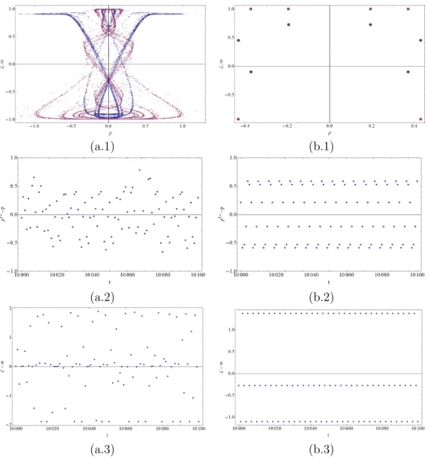
A natural reason to desire a change in the learning rule is if the forecast errors are systematic. FPED can produce systematic and non-systematic forecast errors for the learning rule and the expert manager’s prediction. Simulations show that whether the forecast errors are systematic is dependent on the parameterization of the model. Figure 15 shows examples of non-systematic and systematic forecast errors for a single parameterization of FPED with two different gain parameters. The figures in column (a) depict the non-systematic forecast errors from the expert manager’s prediction when γ = 0.95. The top graph (a.1) plots (pt, mt) and (pt, ζt) to
demonstrate the strange attractor of FPED under this parameterization to illustrate the underlying reason the forecast errors are not systematic, which is mathematical chaos. The plot shows the time path of (pt, mt) and (pt, ζt) for 20,000 periods after
an initial 10,000 iterations of FPED. The last two graphs of column (a) show the forecast errors of the expert managers’ price prediction and the forecast errors of the prediction for the difference in the fraction of predictors chosen over time. The forecast errors for the learning rule appear to almost be white noise (panel (a.3)). The mean forecast error of the learning rule is zero and the first autocorrelation is 0.0776, which suggest there is not a strong empirical reason to alter the rule. The forecast errors of the expert forecast are also mean zero and have a first autocorrelation of 0.2791. Ironically, the higher autocorrelation in the expert managers’ price forecasts provides empirical justification for abandoning rational expectations (CK and CP) over fictitious play learning.
The figures of column (b) show the opposite result for the same parameterization of the model with γ = 0.5. The forecast errors are systematic and the expert manager may indeed wish to alter the forecast rule. This line of reasoning adds a secondary layer of dynamic predictor selection to the model, which further illustrates the complexity of heterogeneous expectations. Further exploration of these issues is interesting, but it is beyond the scope of this paper. My goal is only to provide evidence of the strategic issues that are present in rationally heterogeneous expectations models.
Conclusion
The selection of predictor rules in a model of rationally heterogeneous expectations is inherently motivated by strategic interaction. A firm considers
alternatives to costly rational expectations because there may exist a profit opportunity to use a free naive predictor depending on the other firms’ predictor choices. However, the introduction of an explicit choice of rational or non-rational expectations requires that additional coordination assumptions be made to coordinate agent behavior. The coordinating assumptions remove the underlying strategic justification for the model’s outcomes.
I demonstrate this fact by showing that the standard rational expectations assumptions are insufficient to allow agents to deduce the distributions of predictor rules chosen under certain conditions. The model requires a non-rational agent common prior belief that assigns each agent a predictor rule to choose and which imparts the knowledge of the distribution of predictor rules chosen in the market. Only with this information can a well-defined predictor rule choice be made and a rational expectation calculated. I then show that the rational expectations predictor is not strategically justified in a relevant range of the parameter space, even if agents possess the non-rational agent common prior belief in addition to the common knowledge of rationality. The two results imply that the standard dynamic predictor selection framework that results in chaotic dynamics is not justifiable as the market outcome of competing, strategic, rationally heterogeneous firms.
The introduction of a minimal amount of strategic interaction into the BH model through the introduction of fictitious play is shown to not alter the basic conclusions of the BH model. There still exist rational routes to randomness. Fictitious play actually increases the range of the known parameter space for which these price dynamics are possible. The impact of fictitious play is to change the justification for the price dynamics. The model’s outcomes under Fictitious Play Equilibrium Dynamics are the result of strategic behavior and perpetual miscoordination between firms’ beliefs
of the contemporaneous actions of their competitors and the actual actions taken in the market.
Supplementary Material and Proofs
Theorem 3 Proof: The proof follows closely to the proof of Result 1 from Brock and Hommes (1997) as the two systems are very similar.
i) WhenC = 0 the steady state isE = (¯p,0). The eigenvalues of the system are
−1< λ1 =−b/(b+ 2B)<0 and λ2 = 1−γ < −1. Therefore it is locally stable. ii) ForC > 0, the first eigenvalue is given by
λ1(ζ) = −
b(B+bζ∗(β) + (b+B)T anh(βc/2))
B(b+ 2B +bζ∗(β)) ,
while λ2 remains the same. As β increases from 0 to infinity, ζ∗(β) =T anh(−βc/2) decreases from 0 to -1, which implies that λ1(ζ) decreases from −b/(b + 2B) to
−b/B <1. Thus, the steady state becomes an unstable saddle point for some critical valueβ1. For β=β1, the eigenvalue λ1 =−1, which implies ζ∗(β1) = −B/b.
iii) For β > β1 a 2 - cycle is created as in ARED. The symmetry of the system implies that the 2 - cycle is of the form {(p1, ζ∗),(p2, ζ∗)} where p2 =−λ1(ζ)p1. Let ˆ
p=p1 =−p2>0 and it must be the case that T anh(β/2(2bpˆ2−c)) =−B/b. This equation has a positive solution when β > β1. The local uniqueness and stability of the 2 -cycle are established using the center manifold reduction technique described by Wiggins (1990). The approximate center manifold is
ut+1 = f(ut) = −b B+ (b+B)Tanh c 2 B(b+ 2B) ut+ Ωu 3 t +O[u] 4 where Ω = b 2(b+B)2Sech[c 2] 3 (B(2B+b(2+γ))Cosh[c2]+b(b+B(1−γ))Sinh[c2]) B(b+2B)3(2B+bTanh[c 2]) and is substituted for β1. Stability of the cycle is given by checking that a = 12f00(0) + 13f000(0) > 0, which holds at β1 if b > B. Q.E.D.
Theorem 4 Proof: There are two cases to consider:
Case 1: Suppose that γ = 1 and consider an initial point E1 = (p1, ζ1) 6= E∗. If γ = 1, then ζt+1 = mt and if β = +∞ then mt takes only the values −1 and 1.
The naive predictor is unstable so for any E1 6= E∗ the price will eventually satisfy
|p¯−pt|>(B+b(1+ζt)/2)/(B+b)
p
2C/b, at which pointmt = 1 becauseπt1+1,e > π 2,e t+1. The next period the price is pt+1 and ζt+1 =mt= 1. If the expert prediction has the
highest expected profit and is chosen by all agents, then the system is mapped ontoE∗
becausep1M,t,e +2 = ¯pandζt+2 =mt+1 = 1. This occurs ifb/2¯p2−C > b/2pt+1(2¯p−pt+1), which holds ifpt+1 >(B+b(1+ζt)/2)/(B+b)
p
2C/b. Nowpt+1is the market outcome of all firm using the expert prediction, so either ζt =mt−1 = 1 and pt+1 = ¯pand the system is already at E∗ or ζt = mt−1 = −1, which implies |p¯−pt+1| > |p¯−pt| by b/B >1 and the system is mapped to E∗ in period t+ 2.
Case 2: By Theorem 2 the naive predictor is always chosen when price is in a neighborhood of the steady state and the naive predictor is unstable when b/B >1. The stable arm of the unstable saddle path is defined by the set Esa = {(¯p, ζ)|ζ ∈
[−1,1]}. If the price pt = ¯p, then the naive predictor is chosen and mt =−1. This
follows from the tie-breaking rule assumed in BH, where firms choose to be naive if profits are equal. The naive predictor is chosen every period and the price remains at ¯p. For any initial ζ, the learning rule converges asymptotically to ζ∗ = −1 for 0< γ <1.
The steady state is not globally unstable because for any initial p0 > p
2C/b
with γ0 = 1, the rational predictor will be chosen and the steady state obtained. But for initial points not mapped onto steady state in the next period, there are no paths to steady state. To show that there are no other paths toE∗ consider an initial point
E1 = (p1, ζ1) such that p1 6= ¯p and p0 <(B +b(1 +ζ1)/2)/(B +b) p
2C/b of FPED. Without loss of generality suppose that E1 is one iteration from being mapped onto
E∗ i.e. E1 is the last iterate on a path to E∗. This implies that E1 = (p1,1) since
p1M,t,e +1 = ¯p if and only if ζt = 1. But if ζ1 = 1, then mt−1 and ζt−1 = 1 because
ζt=ζt−1+γ(mt−1−ζt−1), 0< γ < 1, andmt−1 can only take on the values of 1 and
−1. And if ζt−1 = 1 and mt−1 = 1, then p1 = ¯p which is a contradiction. Therefore, there does not exist a path from some E 6=E∗ toE∗. Q.E.D.
(a)
(b)
(c)
(d)
FIGURE 1. Bifurcation diagrams with respect to β. (a) is ARED. (b) is FPED with γ = 0.95. (c) is FPED with γ = 0.5. (d) is FPED with γ = 0.1. The other parameters of the model are A= 0, B = 1, b = 2, C = 0.1.
(a)
(b)
(c)
FIGURE 2. Bifurcation diagrams with respect toγ. (a) is FPED with β = 20. (b) is FPED with β = 60. (c) is FPED withβ = +∞. The other parameters of the model are A= 0, B = 1, b= 2, C= 0.1.
(a.1) (b.1)
(a.2) (b.2)
(a.3) (b.3)
FIGURE 3. The forecast errors of the fictitious play learning rule (2.13) and the expert managers’ predictions for β = 60, A= 0, B = 1, b= 2, C = 0.1 and γ = 0.95 (column (a)) and γ = 0.5 (column (b)). (a.1) and (b.1.) are the attractors of FPED. Both (pt, mt) and (pt, ζt) are plotted. In (b.1) the squares correspond to (pt, ζt).
CHAPTER III
THE INFLATION GAP, FORECAST COMBINATION, AND THE FORECAST COMBINATION PUZZLE
Introduction
Short horizon forecasts of economic measure of the macroeconomy are key inputs into the decision making process of monetary policymakers. The uncertainty surrounding individual forecasts and the plethora of forecasting methods that exist to construct these short horizon forecasts prompt many monetary authorities to consider combined or pooled forecasts.1 The natural question that arises when considering combined forecasts is how the forecasts should be combined to create an optimal or best forecast.
This paper proposes a new dynamic forecast procedure to create combined forecasts of inflation that is shown to consistently and robustly outperform other common forecast combination strategies in root mean squared forecast error (RMSFE) in real-time out-of-sample forecasting exercises. The proposed method combines recent results from the literature on inflation persistence with research that explains the stylized facts that exist in studies of empirical forecasts to create a simple dynamic combination procedure. The combination procedure proposed is general and potentially could improve the forecast efficiency for combined forecasts for any time series of interest, but I restrict the analysis to inflation so as to draw upon a large literature of empirical observations that can explain the increased efficiency obtained. 1Robertson (2000) details the different forecasting strategies employed by a subset of central banks and describes how many explicitly use combined forecasts.
Forecast Combination
Forecast combination or pooling of forecasts is a well-known approach to improve forecast efficiency dating back to the seminal paper of Bates and Granger (1969). This paper launched an entire subfield of econometrics dedicated to explaining the efficiency gains observed from combining forecasts and to devise new schemes to improve efficiency. Surveys of the literature are found in Clemen (1989), Diebold and Lopez (1996), and Timmermann (2006).
A common empirical finding in this literature, including with forecast of inflation (see Stock and Watson (2003)), is that the simple average of the considered forecasts consistently produces the most efficient combined forecasts. The average typically outperforms each individual forecast considered and forecasts generated by more sophisticated combination procedures. The result is found despite the fact that under standard assumptions about the data, equal weights (averaging) is only theoretically optimal under very restrictive assumptions. This empirical finding is called by Stock and Watson (2004), ”the forecast combination puzzle.”
Hendry and Clements (2004) provide details of a generally accepted hypothesis for the existence of the forecast combination puzzle, which is that equal weights provide a hedge against unanticipated structural breaks and misspecification errors that affect the individual forecasts’ efficiencies differently. The majority of the sophisticated weighting strategy proposed in the literature attempt to use past data to choose the combination weight for each forecast. However, the existence of the aforementioned breaks and errors implies that the historical performance of a forecast may not be a guide to its future performance. Employing equal weights is superior in these scenarios because the weights are agnostic about the best forecasts and do
not shift weight to forecasts that have performed well in past, leading to suboptimal forecasts in the future when efficiencies change.2
The literature studying inflation persistence in the U.S. confirms the existence of both frequent structural breaks (Levin and Piger (2006)) and time-varying misspecification in popular econometric forecasts (Stock and Watson (2010)). However, the literature also finds thats the structural breaks and time-varying misspecification are not necessarily unpredictable.
The Inflation Gap
Cogley, Primiceri, and Sargent (2010) and Stock and Watson (2007) both propose parsimonious univariate models of inflation that decompose inflation into a stochastic trend, a serially uncorrelated transitory component, and which allow for stochastic volatility (UC-SV) to study how inflation persistence has changed over time. These studies focus on a measure termed by Cogley, Primiceri, and Sargent (2010) as the inflation gap. The inflation gap is the deviation of inflation from its estimated stochastic trend. These studies find evidence that the inflation gap is predictable using real activity measures, such as GDP and unemployment. Stock and Watson (2010) argue further that the inflation gap can be used to create improved forecasts of inflation.
The inflation gap is the forecast error from the optimal univariate forecast of inflation generated by the UC-SV model. Therefore, one interpretation of the literature’s findings is that the forecast errors of parsimonious forecasting model, which are consistently found to produce the best forecasts of inflation, have time-2A second hypothesis is based on the practical implementation of combination strategies that require additional estimation from past data. The additional parameters add either new sources estimation uncertainty that lead to lower forecast efficiency as found in Smith and Wallis (2009) or contribute to model overfitting.
varying structures that are predictable using real activity measures or other relevant explanatory variables. I explore the possibility that the predicted efficiency could be used to construct intercept corrections of the forecasts similar to those studied in Stock and Watson (2010) or used to pick weights to create an efficient combined forecast. I find that creating combined forecast using the predicted forecast errors of a menu of candidate forecasts can significantly and robustly produce efficient forecasts of inflation that outperform equal weights forecasts and other simple combination strategies in real-time out-of-sample forecasting exercises.
The concept is demonstrated by selecting a list of parsimonious candidate forecast models commonly used in the inflation forecasting literature. I show that the real-time forecast errors generated by the candidate models are serially correlated and can be predicted using real activity measures. I then use the predictions to create combined real-time forecasts for four different measures of inflation.
Predicting Forecast Errors
Stock and Watson (2007 and 2010) consider the following tightly parameterized UC-SV model for inflation:
πt = τt+ηt, whereηt=ση,tζη,t (3.1) τt = τt−1+t, where t=σ,tζ,t (3.2)
lnση,t2 = lnσ2η,t−1+ψη,t (3.3)
lnσ2,t = lnσ2,t−1+ψ,t, (3.4)
where ζt = (ζη,t, ζ,t) is i.i.d. N(0, I2),ψt= (ψη,t, ψ,t) is i.i.d N(0, γI2), and ζt and ψt
time-t forecast of this model is τt|t for all h ≥ 1 and the inflation gap at time t+h
can be defined as at+h =πt+h−τt|t. Stock and Watson posit that the inflation gap is
predictable using real activity measures of the economy such that
πt+h−τt|t=ωhxt+et+h, (3.5)
where xt is vector of real activity measures and et+h is the error term.
The justification for their supposition is that if the stochastic volatility in τt is
ignored, then τt can be written as
τt = (1−θ)
∞ X
i=1
θiπt−i (3.6)
and the inflation gap can be expressed as
πt+h−πt=−θ
∞ X
i=1
θi∆πt−i+ωhxt+et+h, (3.7)
by substituting (3.6) into (3.5). Stock and Watson note that equation (3.7) is just a tightly parameterized backward-looking Phillips curve, which has been a staple of the inflation forecasting literature for decades. They show that this specification is able to augment and improve the forecasts from the UC-SV model compared to other common forecast methods in pseudo out-of-sample forecasts.
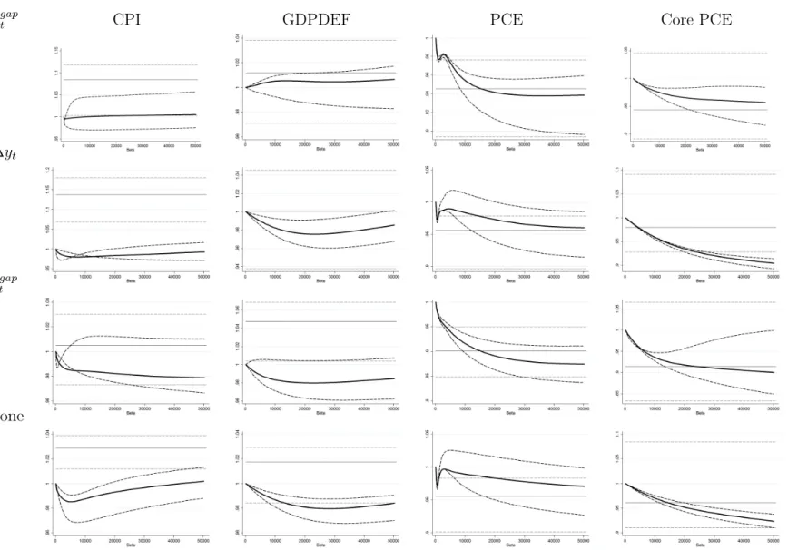
I expand this idea to consider the possibility that the forecast errors of any forecast of inflation are predictable using real activity mea