Essex Finance Centre
Working Paper Series
Working Paper No27: 01-2018
Measuring Dynamic Connectedness with Large
Bayesian VAR Models
“Dimitris Korobilis and Kamil Yilmaz”
Essex Business School, University of Essex, Wivenhoe Park, Colchester, CO4 3SQ Web site: http://www.essex.ac.uk/ebs/
Measuring Dynamic Connectedness with Large
Bayesian VAR Models
Dimitris Korobilis
University of Essex
Kamil Yilmaz
Ko¸c University
January 2018
Abstract: We estimate a large Bayesian time-varying parameter vector autoregressive (TVP-VAR)
model of daily stock return volatilities for 35 U.S. and European financial institutions. Based on that model we extract a connectedness index in the spirit of Diebold and Yilmaz (2014) (DYCI). We show that the connectedness index from the TVP-VAR model captures abrupt turning points better than the one obtained from rolling-windows VAR estimates. As the TVP-VAR based DYCI shows more pronounced jumps during important crisis moments, it captures the intensification of tensions in financial markets more accurately and timely than the rolling-windows based DYCI. Finally, we show that the TVP-VAR-based index performs better in forecasting systemic events in the American and European financial sectors as well.
Key Words: Connectedness, Vector autoregression, Time-varying parameter model, Rolling window
estimation, Systemic risk, Financial institutions.
JEL codes: C32, G17, G21
Corresponding Author: Kamil Yilmaz; Ko¸c University, Rumelifeneri Yolu, Sariyer, Istanbul 34450 Turkey; [email protected]; Tel: +90 212 338 1458; Fax: +90 212 338 1393.
Acknowledgments: For helpful discussions, we thank seminar participants at the University of
Pennsylvania, Mannheim University, Ko¸c University, Universite de Toulouse. We are similarly grateful to participants at the 10th SoFiE Conference in New York University, IAAE in Milan, CFE in Sevilla, and NBER-NSF Time Series Conference in Vienna. We are especially grateful to Francis X. Diebold, Christian Brownlees, Mert Demirer, Umut Gokcen and Han Ozsoylev.
1
Introduction
Financial institutions played a key role in the U.S. financial crisis, both in its earlier domestic phase as well as during its transformation into a global financial crisis. Disproportionate risks taken by big financial institutions have caused over time serious trouble for the global financial system. Therefore, a major challenge for investors and policy-makers alike is to measure these risks in a timely manner and assess their potentially detrimental effects to the wider financial system and the whole economy. Since the outburst of the global financial crisis there has been a plethora of studies that
develop alternative measures of systemic risk. In particular, alternative recent
methodologies that analyze financial firm connectedness, does so exclusively in a
multivariate setting. The equi-correlation approach of Engle and Kelly (2012), for
example, effectively focuses on average pairwise correlations. The CoVaR approach of Adrian and Brunnermeier (2016) and the marginal expected shortfall (MES) approach of Acharya et al. (2017) go beyond pairwise association, tracking association between individual-firm and overall-market movements, in one direction or the other.
In this paper our aim is to make a methodological contribution to the literature on the measurement of systemic risk. In particular, we propose to use a large Bayesian vector autoregressive (BVAR) model with drifting coefficients and stochastic volatility, in order to develop measures of systemic risk. Our methodological approach builds on the recent work of Koop and Korobilis (2013) and introduces several contributions and novel features.
First, we extend the algorithm of Koop and Korobilis (2013) to account for estimation uncertainty of the BVAR covariance matrix. Unlike their algorithm, which can produce only point estimates of covariances and correlations, we propose a Bayesian estimation procedure that fully incorporates parameter uncertainty in the construction of the systemic risk index. Second, we establish that our algorithm is numerically fast
and stable by applying it on daily data and VARs of large dimensions.1
Finally, we establish empirically that our proposed econometric specification is by far the most appropriate for the analysis of volatility connectedness of American and
European financial institutions over time. Our starting point is the Diebold-Yilmaz
Connectedness Index (DYCI) framework; see Diebold and Yilmaz (2014, 2015) for more information. The DYCI framework provides a simple, yet powerful, methodology for measuring and monitoring systemic risk over time. The index measures connectedness
1Our data is both “tall” (many observations) and “fat” (many variables). The fact that we establish
estimation of BVARs with time-varying parameters using such data, is an empirical success on its own merit. Such models typically assume random walk evolution of parameters and, hence, are subject to “exploding” coefficients and numerical instability; see the discussion in Primiceri (2005, Section 4).
based on the decomposition of the forecast error variances in a vector autoregression. The framework also allows the measures of connectedness to change over time, which enables the user to track it as a dynamic measure of systemic risk.
Nevertheless, the dynamic connectedness measures in the original work of
Diebold-Yilmaz are obtained through the use of rolling-sample estimation of the VARs, based on a fixed window of observations. The use of rolling windows in order to obtain variance decompositions and, hence, connectedness measures, has its own limitations. For instance, from an econometric point of view, rolling estimation means that valuable information from the sample is discarded. Most importantly, from the point of view of economic interpretation of the index, rolling window estimations results in “built-in
persistence” in the dynamic connectedness index. By this we mean that, while the
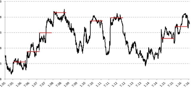
resulting DY volatility connectedness index does rightfully capture the increase in connectedness when there is a sizeable volatility shock to one or more of the members of the system, it does not necessarily capture the downward move in connectedness in a timely manner as the effect of the shock dissipates over time. To the contrary, as can be seen from Figure 1, the index tends to stay high as long as the observation that pertains to the day of the shock is included in the fixed-length rolling-sample window. This generates an over-estimation of both total, total directional, and pairwise connectedness measures after major financial shocks and other episodes.
68 73 78 83 88 93
Figure 1: Excessive persistence in total connectedness with 200-day rolling window In Figure 1, such excessive persistence is especially visible during the first and second European banking and sovereign debt crises of May 2010 and August 2011. One can also identify persistence of the index during several important turning points of the 2007-2008 U.S. financial crisis (August 2007 liquidity crisis, unscheduled meeting of the Federal
Open Market Committee (FOMC) to lower policy interest rates twice in January 2008 and the collapse of Lehman Brothers in mid-September 2008), as well as following the London bombings on July 7, 2005 and FOMC’s unexpected policy interest rate hike on May 10, 2006, the U.S. bond market flash crash in mid-October 2014 and August 2015 financial market troubles in China. We, therefore, argue that a more carefully specified econometric model, can be quite instrumental in overcoming the major obstacle in the accurate measurement of connectedness across assets and/or financial institutions. By allowing VAR parameters to vary over time, the proposed TVP-VAR model relieves the researcher from the necessity to roll a fixed-length sample window in order to capture the dynamics of the connectedness. The methodology we propose incorporates the benefits of Bayesian shrinkage for estimating high-dimensional systems, without the need to rely on computationally intensive simulation methods. The resulting dynamic connectedness index and the directional connectedness measures would not be subject to the persistence observed in the rolling-sample windows estimation.
In the rest of the paper we proceed as follows. In section 2, we summarize the
estimation of large TVP-VARs as the empirical approximating model for the unvocer the underlying connectedness model in the DYCI framework. In section 3, we briefly
summarize the Diebold-Yilmaz connectedness-measurement framework. In section 4,
we provide the information about financial institutions that we include in our analysis as well as the range volatilitiy estimates. In section 5, we present the dynamic total and directional volatility connectedness indices and discuss their behavior over time in comparison with the corresponding measures obtained from rolling windows estimation framework. In the same section, we analyze the change in the structure of the volatility network during important crisis episodes. We conclude in section 7.
2
An Adaptive Estimation Algorithm for TVP-VAR
Models
As we have discussed in the Introduction, our main objective in this paper is to remedy one of the shortcomings of the Diebold-Yilmaz framework, namely excessive persistence of the connectedness measures following a significant shock to the system. Instead of estimating the VAR model over rolling sample windows, which results in discarding valuable observations, we propose to estimate a time-varying parameter VAR model over the full sample. Here we provide a short description of a simple adaptive algorithm for the estimation of TVP-VAR models of large dimensions. This algorithm is “online” meaning that as new data become available, one can simply update parameter estimates
at time t using only estimates at time t−1, that is, without the need to use the full sample each period (which would be computationally costly).
We start with the specification of the following time-varying parameter VAR(p) model:
yt =ϕ0t+ Φ1tyt−1+...+ Φptyt−p+εt,
where εt ∼N(0,Σt) with Σt an M ×M covariance matrix. Consider the K ×1 vector
βt = vec
ϕ00t,Φ01t, ...,Φ0pt0 where K = M(1 +M p) and define the M ×K vector
xt=I⊗
1, y0t−1, ..., yt0−p. When limited information is available about the exact nature
of parameter changes, the vector of coefficientsβt are usually allowed to follow a random
walk2 of the form so the TVP-VAR can be represented as
yt = βtxt+εt,
βt = βt−1 +ηt,
where ηt ∼ N(0,Ωt) and Ωt is a K ×K covariance matrix. While such state-space
formulations have been used extensively in economics, the main challenge in large dimensions is how to track parameter evolution with a low computational cost. Existing Bayesian Monte Carlo or maximum likelihood algorithms allow updates of the
covariance matrices Σt and Ωt that can become numerically unstable and
computationally demanding in larger dimensions; see discussion in Koop and Korobilis (2013).
We follow a computationally simple solution in order to track parameters in real time.
First note that if Σtand Ωt are known, then the Bayesian solution to learning about the
coefficients βt takes the form
p(βt|Dt) ∝ L(yt;βt, xt,D1:t−1)p(βt|Dt−1)
p(βt|Dt−1) =
Z
℘
p(βt|D1:t−1, βt−1)p(βt−1|Dt−1)dβt
where Dt = (yt, xt), D1:t denotes all data for periods 1 to t, and ℘ is the support of βt.
This tracking problem can be solved trivially with a single run of the Kalman filter. It is
only when Σt and Ωt are unkown that simulation methods have to be used, e.g. MCMC
as argued above, or the EM algorithm of Shumway and Stoffer (1982), or importance sampling as in Uhlig (1997). In this paper we follow Koop and Korobilis (2013), Prado and
2 A random walk process can capture richer patterns in the evolution ofβ
tcompared to a stationary
autoregressive process, and has been popular in economics at least since Cooley (1971). Additionally, Sims (1989) finds that even when an AR(1) process is assumed forβtin a typical VAR, the autoregressive
West (2010), and Dangl and Halling (2012) and consider the idea of variance discounting. In this case we set
Ωt = 1−λ−1
var(βt|Dt−1),
where at time t the filtered covariance matrix var(βt|Dt−1) is readily available from the
Kalman filter. The quantity 0 < λ ≤ 1 is a decay factor which controls how fast the
time-variation occurs inβt. In practice this specification implies that an effective window
size of EW = 1/(1−λ) observations is used for estimation. Thus as λ gets lower, less
observations are used for estimation ofβt, which implies that older data are discounted at
a faster rate andβtcan vary substantially from one period to the next. In the extreme case
λ= 1 we can see that Ωt= 0 in which case βt=βt−1 for allt, i.e. βt becomes a constant
parameter, therefore, our model can nest traditional constant parameter BVARs. Given
that the discount rateλ can be interpreted as a prior for the amount of time-variation in
parameters, we present in the Appendix an adaptive procedure to estimate λ from the
data.
Regarding estimation of the VAR covariance matrix, we follow Uhlig (1994), Uhlig (1997) and Prado and West (2010) and define the following Beta matrix evolution model:
Σt=Ut0−1BtUt−1, (1)
where Ut−1 denotes the upper triangular matrix of the Choleski decomposition of Σt−1,
and Bt is a scaled version of a matrix-variate “inverse beta” distribution. This
particular evolution from Σ−t1 = Ut0−1Ut−1 to Σt as defined above means that the
posterior distribution of Σt is inverse Wishart; see West and Harrison (1997) for more
details. Given the evolution of the covariance matrix specified in equation (1), we follow
Triantafyllopoulos (2007) and derive the implied prior and posterior for Σt when βt has
an independent (non-conjugate) prior. It can be shown that the time t prior of the
covariance matrix is of the form
Σt|Dt−1 ∼iW St|t−1, nt|t−1
(2) and the resulting posterior is
Σt|Dt ∼iW(St, nt) (3)
where iW denotes the inverse Wishart distribution, and exact expressions for the scale
3
The Connectedness Index Methodology
After providing a description of the TVP-VAR model, in this section we briefly describe the Diebold-Yilmaz connectedness index methodology, which is developed in a series of papers (Diebold and Yilmaz, 2009, 2012, 2014).
DYCI is obtained from the variance decomposition matrix associated with a covariance
stationaryN-variable vector autoregregression (VAR(p)). Variance decompositions allow
one to split the forecast error variances of each variable into parts attributable to the various system shocks. As such, variance decompositions also allow one to assess the
fraction of the H-step-ahead error variance in forecasting xi that is due to shocks to
xj,∀i6=j, for each i.
Standard variance decompositions based on Cholesky factorization depend on the
ordering of the variables, significantly complicating the study of directional
connectedness. Hence, Diebold and Yilmaz (2012) suggest exploiting the generalized VAR framework of Koop et al. (1996) and Pesaran and Shin (1998), which produces variance decompositions invariant to ordering. Instead of attempting to orthogonalize shocks, the generalized approach allows correlated shocks but accounts for them appropriately using the historically observed distribution of the errors. As the shocks to each variable are not orthogonalized, the sum of contributions to the variance of forecast error (that is, the row sum of the elements of the variance decomposition table) is not necessarily equal to one.
The generalized impulse response and variance decomposition analyses also rely on
the MA representation of the N-dimesnsional VAR(p). Pesaran and Shin (1998) show
that when the error termεthas a multivariate normal distribution, theh-step generalized
impulse response function scaled by the variance of the variable is given by:
γjg(h) = √1
σjj
AhΣej, h= 0,1,2, ... (4)
where Σ is the variance matrix for the error vectorε,σjj is the standard deviation of the
error term for the jth equation and ei is the selection vector with one as the ith element
and zeros otherwise. Variable j’s contribution to variable i’s H-step-ahead generalized
forecast error variance, θgij(H), for H = 1,2, ..., is defined as:
θijg(H) = σ −1 jj PH−1 h=0(e 0 iAhΣej)2 PH−1 h=0(e 0 iAhΣA0hei) (5) As explained above, the sum of the elements of each row of the variance decomposition
table is not necessarily equal to 1: PN
j=1θ
g
ij(H)6=1. In order to use the information
Diebold and Yilmaz (2012) normalize each entry of the variance decomposition matrix
(equation 5) by the row sum as3:
˜ θgij(H) = θ g ij(H) PN j=1θ g ij(H) (6) Now, by construction PN j=1θ˜ g ij(H) = 1 and PN i,j=1θ˜ g
ij(H) = N. Using the normalized
entries of the generalized variance decomposition matrix (equation 6), Diebold and Yilmaz (2012) construct the total connectedness index as:
C(H) = PN i,j=1 i6=j ˜ θgij(H) PN i,j=1θ˜ g ij(H) = PN i,j=1 i6=j ˜ θijg(H) N (7)
Next considering directional connectedness, Diebold and Yilmaz (2012) define gross
directional connectedness received by bank i from all other banks j as:
Ci←• = PN j=1 j6=i ˜ θijg(H) PN i,j=1θ˜ g ij(H) ×100 = PN j=1 j6=i ˜ θijg(H) N ×100 (8)
In similar fashion, directional volatility connectedness transmitted by banki to all other
banks j is measured as:
C•←i = PN j=1 j6=i ˜ θjig(H) PN i,j=1θ˜ g ji(H) ×100 = PN j=1 j6=i ˜ θjig(H) N ×100 (9)
One can think of the set of directional connectedness as providing a decomposition of total connectedness into those transmitted by each bank in the sample. Obviously, once
the financial shocks transmitted and received by bank i are calculated, the difference
between the two will result in a measure of the net directional connectedness transmitted
from bank i to all other banks as:
Ci(H) = C•←i(H)−Ci←•(H) (10)
The net directional connectedness index (equation 10) provides information about how much each financial institution’s stock return volatility contributes in net terms to stock return volatilities of other institutions.
Diebold and Yilmaz (2014) showed that the connectedness framework was closely
linked with the modern network theory. To start with, they showed that the total
3Alternatively, one can normalize the elements of the variance decomposition matrix with the column
sum of these elements and compare the resulting total connectedness index with the one obtained from the normalization with the row sum.
connectedness measure corresponds to the mean degree of a weighted, directed network. They also showed that the connectedness framework was closely linked to the modern
measures of systemic risk. For example, the from-connectedness degree measures
exposures of individual banks to systemic shocks from the network, in a way very much similar to the marginal expected shortfall of these banks (Acharya et al. (2017)). The to-connectedness degree, on the other hand, measures the contribution of individual banks to systemic network events, in a fashion very similar to CoVaR of the bank (Adrian and Brunnermeier (2016)).
4
Construction of Stock Return Volatilities
Financial institutions can be connected with each other through several channels. These channels could include counter-party linkages associated with positions in various assets, contractual obligations associated with services provided to clients and other institutions, and deals recorded in their balance sheets. High-frequency analysis of financial institution connectedness therefore might seem to require high-frequency balance sheet and related information, which is generally unavailable.
Fortunately, however, data on stock prices are available. Following Diebold and
Yilmaz (2016) we use individual stock price data to obtain range-based stock return
volatility estimate, which has received significant attention in recent years.4 For a given
financial institution on a given day, we construct a daily range-based volatility estimate
using the natural logarithms of daily high (h), low (l), opening (o) and closing (c)
prices, ˜
σ2gk = 0.511(h−l)2−0.019[(c−o)(h+l−2o)−2(h−o)(l−o)]−0.383(c−o)2,
as proposed by Garman and Klass (1980).
We study stock return volatilities of 35 major financial institutions; 17 of these are
American financial institutions while the remaining 18 are European. The sample
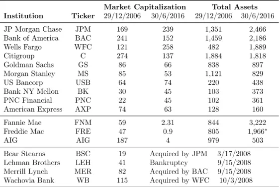
covers 2 January 2004 - 22 July 2016 with 3235 daily observations. In Tables 1 and 2 we show the US and EU financial institutions, respectively, along with their stock tickers, stock market capitalization and total assets in the pre-crisis period (29 December 2006) and at the end of the sample (30 June 2016 for U.S. banks and 31 March 2016 for the European banks). The US sample includes 8 commercial banks, 5 investment banks,
two mortgage companies, one credit card company and one insurance company.5 The
4 On range-based volatility, see, for example, Alizadeh et al. (2002).
5 The US sample includes stocks of 7 financial institutions that were either acquired by another
Table 1: U.S. Financial Institution Detail (bn. US$)
Market Capitalization Total Assets
Institution Ticker 29/12/2006 30/6/2016 29/12/2006 30/6/2016
JP Morgan Chase JPM 169 239 1,351 2,466
Bank of America BAC 241 152 1,459 2,186
Wells Fargo WFC 121 258 482 1,889 Citigroup C 274 137 1,884 1,818 Goldman Sachs GS 86 66 838 897 Morgan Stanley MS 85 53 1,121 829 US Bancorp USB 64 74 220 438 Bank NY Mellon BK 30 45 103 373 PNC Financial PNC 22 45 102 361
American Express AXP 74 63 128 160
Fannie Mae FNM 59 2.31 844 3,222
Freddie Mac FRE 47 0.9 805 1,966∗
AIG AIG 187 4 979 503
Bear Stearns BSC 19 Acquired by JPM 3/17/2008
Lehman Brothers LEH 41 Bankruptcy 9/15/2008
Merrill Lynch MER 82 Acquired by BAC 9/15/2008
Wachovia Bank WB 115 Acquired by WFC 10/3/2008
Notes: Freddie Mac’s total assets are as of 31 March 2016.
European sample consists entirely of commercial banks.6 The vast majority of the
included financial institutions, whether US or European, are classified as Global
Systemically Important Banks (G-SIBs).7
Market capitalization of all US financial institutions included in the full-sample analysis declined substantially during the global financial crisis. Since the end of the global financial crisis in the first half of 2009, their stock prices recovered some of the
lost ground. As a result, as of 30 June 2013, market capitalizations of 5 out of 10
relatively healthy US financial institutions were either above or very close to their corresponding market capitalizations on 29 December 2006. Five banks that have lower market capitalization in 2016 compared to 2006 are Bank of America, Citigroup,
Goldman Sachs, Morgan Stanley and American Express. Troubled US financial
institutions, Fannie Mae, Freddie Mac and AIG, suffered substantial declines in the
market capitalizations in since 2006. These institutions are not included in our
connectedness analysis since the end of 2008, along with those banks that cease to exist taken under government custody (Fannie Mae, Freddie Mac and AIG). We include those stocks from the beginning of the sample until the time they went bankrupt, were taken over by another financial institution, or taken into government custody.
6 Only one of the European institutions, Dexia, was taken over to the custody of the Belgian and
French governments.
7 Of the 27 financial institutions that are included in the full-sample, only six (three from the US,
three from the EU) are not included in the G-SIBs list announced by the Financial Stability Board on 1 November 2012.
Table 2: EU Financial Institution Detail (bn. US$)
Market Capitalization Total Assets
Institution Ticker Country 29/12/2006 31/3/2016 29/12/2006 31/3/2016
Dexia DEX Belgium 31 40 567 266
KBC KBC 45 25 325 298
Deutsche Bank DBK Germany 70 35 1,584 1,980
Commerzbank CBK 25 11 608 610
BNP Paribas BNP France 101 69 1,440 2,413
Societe Generale GLE 79 33 957 1,556
Credit Agricole ACA 63 27 1,260 1,793
Unicredit Group UCG Italy 91 20 823 1,015
Intesa San Paolo ISP 46 43 292 797
ING Bank ING Netherlands 98 48 1,226 988
Bank Santander SAN Spain 117 69 834 1,506
BBVA BBVA 85 43 412 843
UBS UBS Switzerland 128 60 2,346 1,006
Credit Suisse Group CSG 85 27 1,255 847
HSBC HSBA UK 211 129 1,860 2,595
Barclays BARC 93 45 997 1,793
Royal B. Scotland RBS 123 42 871 1,267
Lloyds Bank LLOY 63 75 344 1,183
either due to bankruptcy or takeover/merger by another bank company.
On the European side, our analysis covers 18 European banks; 16 of these are from 7 EU member countries while the remaining two are from Switzerland (see Table 2). The European sample is not complete without the two big Swiss financial institutions, namely UBS and Credit Suisse Group. All European banks in our sample, except for Lloyds and Dexia, are valued lower by the market at the end of March 2016 compared to the end of 2006. While their market values went down in the last ten years, majority of the European banks experienced significant increases in their total assets.
5
Empirical Results
Our key empirical result concerns the comparison of the dynamic total connectedness indices from VAR model estimated over rolling-sample windows and the TVP-VAR model with Minnesota prior estimated over the full sample. Before comparing the two estimates, however, we first present the TVP-VAR model evidence alone and follow its behaviour over time.
Once we carefully analyze the time series behavior of the TVP-VAR model based connectedness index, we go ahead and compare this index with the one based on the
VAR model estimated over a 200-day rolling window. The difference between the two graphs are crystal clear. The TVP-VAR model based connectedness index definitely displays a larger number of upward increases than the RW-VAR based connectedness index. We interpret this result as the TVP-VAR based index capturing the impact of critical economic, political and other developments that affected the European and the U.S. financial systems, in general, their respective banking industries, in particular.
In the closing part of this section we present plots that show that our TVP-VAR based connectedness index is not sensitive to parameter choices and the results presented in Figure 2 will go through when we consider alternative specifications.
5.1
TVP-VAR Based Connectedness Index Over Time
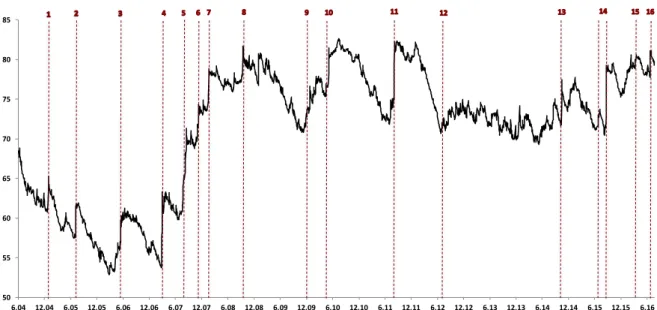
In Figure 2 we plot the connectedness index from our base TVP-VAR model with Minnesota prior. The graph identifies a total of 16 jumps in the volatility connectedness index, all of which are indicated with red labels. As can be seen in Table 3 all jump episodes in the TVP-VAR-based dynamic connectedness index (in Figure 2) correspond to major financial, economic and/or political events that had significant impact on financial markets over the period from 2004 to 2016.
The first significant increase in the index is relatively small compared to increases during some of the subsequent major events (see Table 3, event #1). It is due to the earthquake that hit the South East Asia on December 26, 2004 and the Great Indian Ocean Tsunami that hit the coastal areas killing approximately 250,000 individuals in several countries. As the resulting damage to the insured property and human lives meant a huge increase in the liabilities of insurance companies (reaching as high as $13 billion, Walker (2005)), financial stocks led by insurance companies were down on December 27 through 29. The resulting increase in the index is slightly higher than 6 percentage points.
The second major shock to banking stocks took place on July 7, 2005, when a series of coordinated terrorist suicide bomb attacks hit the central London area (event #2). As the July 7 2005 observation is taken into account the estimated parameters of the VAR model respond such that the resulting connectedness index jumps more than 10 percentage points. However, the index declines quickly immediately afterwards falling below the pre-July 2005 level before the end of 2005.
The third major jump in the index started in May 2006 and continued in June 2006
(event #3). In May 2006, the Federal Reserve’s Federal Open Market Committee
(FOMC) decided to increase the policy interest rate from 4.75% to 5.0% with an announcement that it was likely to increase the rate a quarter of one percent in its subsequent meeting in June 2006. As the announcement caught the financial investors
50 55 60 65 70 75 80 85 6.04 12.04 6.05 12.05 6.06 12.06 6.07 12.07 6.08 12.08 6.09 12.09 6.10 12.10 6.11 12.11 6.12 12.12 6.13 12.13 6.14 12.14 6.15 12.15 6.16 In de x
Figure 2: Total Connectedness from TVP-VAR Model
off guard, there was a significant reaction to it. It effectively led to a quick unwinding of the dollar carry trades in many emerging market economies, simulatenously affecting bank stocks on both sides of the Atlantic. As a result of the increase in bank stock return volatilities, the TVP-VAR model based index increases by around 10 percentage points from 57% in late April to in 67% in mid June 2006. As the impact of higher U.S. interest rates reverbated around developed and emerging market economies, the index did not come down as quick as the previous two upward moves of the index.It took approximately 6 months for the index to decline to levels commensurate with the pre-May 2006.
The impact of the next major event on the index was even more pronounced. It took place in late February and early March 2007 (event #4). The first signs of the U.S. subprime crisis were observed in February 2007, beginning with HSBC’s well-publicized
exit from the mortgage markets in the U.S. at a $10.6 billion loss. In addition,
Countrywide Financial announced that 20% of the subprime loans they serviced were late with payments. The bad news from the mortgage markets combined with the 9% drop in Chinese stock markets a day earlier and the more-than-expected drop in U.S. durable goods demand, led to a 3.3% (415 points, biggest drop after the 9/11 terrorist attacks in 2001) drop in Dow Jones Industrials Average on February 28, 2007. The connectedness index jumped 16 percentage points in three days from February 26 to March 1, 2007. However, different from previous cases, after this substantial shock the index declined very little.
Then came the liquidity crisis of August 2007, when the liquidity in the U.S. and European financial markets dried very quickly when BNP Paribas decided to halt
Table 3: Chronology of Events Affecting U.S.-European Bank Volatility Connectedness
No Event Detail
1 December 26, 2004: South East Asia earthquake and the Great Indian Ocean Tsunami;
financial stocks led by insurance companies were down on December 27 through 29, 2004.
2 July 7, 2005: London bombings
3 May 10, 2006: FOMC decision to increase FFR target, massive unwinding of carry trades.
4 Feb 27, 2007: First tremors of the subprime crisis; 3 mortgage originators filed for bankruptcy.
5 July 20 - August 20, 2007: Liquidity Crisis.
6 October-November 2007: Major US banks announced big losses for the 3rd quarter;
several CEOs resigned.
7 January 2008: Bad news from financial markets around the world; FOMC had to meet
twice in a week to lower rates
8 September 15, 2008: Lehman Brothers’ collapse followed by massive capital injection to AIG and major commerical banks in the U.S.
9 Mid-Oct. – mid-Dec. 2009: Big hole in the Greek government budget announced, followed by
Greek sovereign debt downgrades to junk status.
10 April-May 2010: Greek debt crisis intensified, with rescue package announced along with austerity measures which led to violent protests in Athens.
11 July-August 2011: News reports about the sovereign debt troubles of Italy and Spain, followed by ECB’s stress test results’ announcement increased the pressure on European banks 12 July 2012: The public became aware of the breadth of the Libor fixing scandal.
13 October 15, 2014: US bond market flash crash
14 June 29 and Aug. 28, 2015: Worries about the Chinese financial sector led to sharp declines in stock market indices around the world.
15 January-February 2016: Deutsche Bank Coco bonds trouble
16 June 24, 2016: Brexit – G. Britain decided to exit from the EU.
redemptions from three of its hedge funds (event #5). From late July to early August, the index jumped more than 15 basis points. After a brief and small correction the index jumped up another 5 points in late October-November as major U.S. banks started announcing billions of dollars of losses in their financial statements for the third quarter of the year (event #6). After a two-month hiatus, during which it came down a couple of percentage points, the index jumped close to 10 points in the first three weeks of January 2008, as bad news were coming in from both the European and the U.S.
banks one after the other (event #7).8
In two months time, Bear Stearns, the weakest member of the top five investment banks, was in the brink of bankruptcy. When the news came out on March 17, the index recorded another three percentage point jump. In response, the New York Fed orchestrated a successful takeover of Bear Stearns by J. P. Morgan, and which helped reverse the earlier jump in the index. The Bear Stearns incident did not create a major impact (nothing more than a minor hick up) on the connectedness index.
8 The news were so bad that the FOMC was forced to hold an unscheduled meeting on January 22,
where it lowered Fed funds rate target rate by 75 basis points. Eight days later, on its scheduled meeting FOMC lowered the policy rate by another 50 basis points.
After the Bear Stearns incident markets stayed relatively calm for a couple of months. As a result, the index declined dring this period, followed by another small hick up in July, due to the troubles of Wachovia Bank.
The more critical and significant jump took place in September (event # 8). First, the worsening in the balance sheets of the Fannie Mae and Freddie Mac, two government sponsored enterprises, had an impact on market volatility at the beginning of September. The index increased from 77.8% on September 5, 2008 to 80.1% on September 9. As a result of these developments, over the weekend of September 6-7 the U.S. Federal Housing Finance Agency (FHFA) decided to take both firms into its conservatorship. This decision brought calm to markets for a couple of days and the index declined slightly to 79.2% on September 12.
Over the weekend of September 13-14, officials from the U.S. Treasury, Federal Reserve and CEOs of major banks met in New York to put together takeover deals to save the most troubled U.S. financial institutions, namely, Lehman Brothers, Merrill Lynch and Wachovia. Despite their best efforts, they were unable to find a suitor for Lehman Brothers. On Monday, September 15, 2008, Lehman Brothers announced its bankruptcy and the hell broke loose. With the bankruptcy of Lehman Brothers, the
U.S. financial crisis was transformed into a global one. The index jumped by 4
percentage points on September 15, followed by 1.5 percentage point increase on the next day. The U.S. Treasury which refused to bail out Lehman Brothers with much less, ended up channeling a total of $126 billion to bail out AIG, the insurance giant that effectively insured Lehman’s debt along with others through what became known as the credit default swaps (CDSs).
The market calmed briefly and the index went gradually down to 79% in the second half of October, but there were widespread rumors about other financial institutions to follow in the footsteps of Lehman and AIG. As a result the index went up again, from 78.5% in early November to 80.8% on November 21. As the Citigroup came close to the brink of collapse, on November 23 the U.S. government decided to invest $20 billion in Citigroup (on top of the $25 billion it had already invested from Troubled Asset Relief Program (TARP) on October 14).
After another slight increase in early February, the index continued its decline until mid-April 2009. As the stress test results announcement date for 19 largest U.S. bank holding companies came closer, the rumors about the possibilities led to an increase in the volatility of the major U.S. bank stocks. As a result, from a low of 75% on April 13, 2009, the index started moving up, reaching its local maximum of 81% on May 7, when the stress test results were released. The stress test results were better than expected: 9 of the top 19 banks had adequate capital, while the remaining 10 banks had to raise
$75 billion in extra capital. After this good news about the health of the U.S. banking sector, the volatility connectedness index continued its downward slide, hitting a low of 70% by mid-Ocober 2009.
That is the time period when the U.S./global financial crisis was transformed into a European sovereign debt and banking crisis (event # 9). On October 16, 2009 the Greek prime minister George Papandreu publically announced that Greek government budget deficit and debt stock situation was actually was worse than announced by his predecessor. George Papandreou’s new socialist government says the 2009 budget deficit would be 12.7 percent of GDP – more than double the published figure by the previous government.
As the accurate information about Greece’s sovereign debt stock was made public, the Greek crisis started to have its impact on European financial markets. From November onwards the Greek debt crisis started to consummate the daily meetings of euro area officials. In December three rating agencies downgraded the Greek sovereign debt credit rating (Fitch on December 8, S&P on December 16 and Moody’s on December 22). From a low of 68.5% on October 20, the connectedness index climbed to 77% by December 10, 2009.
Greece’s troubles continued in early 2010 as an ECB report revealed how bad the economic situation was in Greece. On February 11, the EU urged Greek government to make further spending cuts while also promising to help Greece to tackle its debt problem. The government’s austerity plans spark strikes and riots in the streets of Athens. Furthermore, concerns started to build about other heavily indebted countries in Europe, namely Portugal, Ireland, Italy, and Spain (making PIIGS). As a result, the index climbed from 75.8% on January 13 to 82.8% on February 23, 2010.
Austerity measures put in effect by the Papandreu government as well as the IMF and ECB’s efforts to put together an emergency fund to help Greece, calmed the markets down and the connectedness index went down 4.5 percentage points in March and the first half of April. Yet, on April 16, there was an uproar of protests in Greece against the government’s request for a 45 billion euros IMF-ECB bailout. The index jumped 3 percentage points on the same day.
Things got even worse on May 2, 2010, when the European Central Bank (ECB), European Commission and International Monetary Fund (IMF), the so-called Troika,
announced ae110 billion bailout loan package to make sure that the Greek government
will not default on its debt, conditional on the implementation of structural reforms and austerity measures. The Troika’s announcement was immediately followed by anti-austerity street demonstrations in Athens. Three people were killed on May 5 in one of the largest street demonstrations in Athens, one day before a critical session in the
parliament about the government’s austerity the city. As a result, the index, which stood at 81 % on May 3, jumped 5 percentage points in the next three days to reach 86% on May 6. (event #10)
After going up one percentage point in July, the index started a downward slide,
which lasted close to a year despite several smaller upward moves.9 Once it hit the
pre-Greek crisis levels in the early summer of 2011, the news about the troubles of Italian and Spanish government debt started to put pressure on financial markets in Europe and around the world. Commensurate with these developments the index went up in two steps: first, five percentage points in the first half-July, which was followed by a 10 percentage point increasein the first week of August, following the EU announcement indicating that the debt rescue planning for Spain, Italy and Cyprus was not on the cards (event #11).
After the second round of the European sovereign debt and banking crisis, the markets calmed down much faster than the first round in 2010. One of the important reasons for this was the significant change in the Euro area monetary policy following the replacement of Jean-Claude Trichet by Mario Draghi as the President of the European Central Bank on November 1, 2011. Starting with the announcement of the Long-Term Refinancing
Operation (LTRO), through which the ECB provided e1 trillion to the Euro Area banks
over a three year period, ECB implemented preemptuive policies to ease the pressure over the Euro Area banks. This policy paid off immediately: the connectedness index declined from 84% at the end of 2011 to 67% by mid-2012.
From July 2012 onwards, the connectedness index started following a longer term upward trend thanks mostly due to the Libor fixing scandal about which the first news reports were published in March 2011. In July 2012, following the $ 450 mn. fine on Barclays by the UK’s regulators made the public became aware of the extent of the crisis. Later in December 2012 UBS was fined $1.5 billion by the US, UK and the Swiss
regulators, followed by the $ 1 billion fine on Dutch Rabobank (October 2013) ande1.7
billion on Deutsche Bank, RBS and Societe Generale by the EU authorities in December 2013) and a $ 2.5 billion fine on Deutsche Bank in April 2015 (event # 12).
The Libor fixing scandal and the subsequent announcements of official fines were responsible for the upward trend in the connectedness index from 2012 through 2013 and even to 2015 as Deutsche Bank had become the last bank to be fined in April 2015.
On October 15, 2014, there was a flash crash in the U.S. sovereign bond markets when the yield on the US 10-year note fell 34 basis points from 2.2% to as low as 1.86% in a matter of several minutes. According to market participants “the volatility seen
9 In March 2011, for example, the index went up a couple of percentage points as the first news
reports about an official probe against several major international banks for Libor rate manipulations were published.
in markets that day has been surpassed only once in the past 50 years.” As a result, the connectedness index jumped by 4.5 percentage points on the same day, followed by another 3 percentage points increase the next day (event # 13).
Within less than two months the emerging stock markets were hit by a plunging Russian rouble against hard currencies following the rapid decline in oil prices. At the same time, the increased troubles in emerging stock markets raised some concerns about the possibility of toruble in Chinese financial markets. The volatility of the European and US bank stocks increased in the second half of December 2014, leading to an increase in the connectedness index to the levels it attained in mid-October due to the flash crash in the US government bond market.
In late June 2015, the global financial markets started to bounce back and forth, as bad news from the Chinese private loan markets increased the tensions about a possible meltdown in Chinese financial markets. As the authorities were not able to in place were not successful in stemming the tide against the Chinese markets, investors’ anxiety led to an even bigger
On February 8, 2016, Deutsche Bank’s market value dropped by 2 billion euros, along with a drop in the value of its coco bonds. Other Eurozone banks also experienced a drop in the value of coco bonds they issued. On February 8 and 9, the connectedness index went up by 2 percentage points. The increase in the index was directly a result of the coco (short for ”contingent convertible”) bonds trouble of Deutsche Bank (event # 15).
10
Finally, on June 23, 2016, to the surprise of many British and EU leaders, 52 percent of British citizens who participated in the referendum voted in favor of leaving the EU. As the majority of the polls predicted a victory for the “stay” camp, it was a major surprise for financial markets as well. On June 24, the Britisih Pound plunged by 8.4 percent to hit a 30-year low, while FTSE 100 index of shared dropped by 3.2 percent for the day (event # 16).
5.2
TVP-VAR versus VAR with Rolling Windows
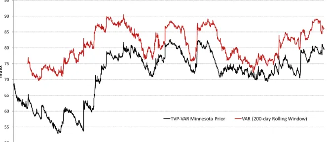
In Figure 3 we plot the connectedness index from our base TVP-VAR model along with the one from the VAR model estimated over 200-day rolling windows. The correlation between the two indices, 0.74, indicates that the overall behavior of the two indices over
10The so-called coco bonds are hybrid securities that were issued by large commercial banks to bolster
the capital base. In order to enhance stability of the banking system, financial regulators in Europe and the US encouraged banks to issue coco bonds, which are converted to equity or are written down when a banks capital falls below a certain level. However, as Deutsche Bank’s experience in February 2016 showed clearly, a sell of in the coco bonds market could actually lead to higher market volatility threatening banks’ market value.
the full sample are not too much different. Despite that fact, the TVP-VAR model based connectedness index (TVP-VAR index, from here on) differs from the rolling windows VAR model based index (RW-VAR index, from here on) in several dimensions.
50 55 60 65 70 75 80 85 90 95 6.04 12.04 6.05 12.05 6.06 12.06 6.07 12.07 6.08 12.08 6.09 12.09 6.10 12.10 6.11 12.11 6.12 12.12 6.13 12.13 6.14 12.14 6.15 12.15 6.16 In de x
TVP-‐VAR Minnesota Prior VAR (200-‐day Rolling Window)
Figure 3: Total Connectedness: TVP-VAR vs VAR with 200-day Rolling Window To start with, the jumps in the TVP-VAR index tend to be more frequent and bigger than the ones observed in the RW-VAR index. This is true for all major events that had a significant impact on the US and European banking sectors: July 5, 2005 terrorist bomb attacks in London, reaction of markets to FOMC decision to increase rates in May and June 2006, the build up of the tensions in the US financial system from early 2007 to turn into a global financial crisis in late 2008, Greek sovereign debt crisis of late 2009 to May 2010, the European sovereign debt and banking crisis of the summer 2011, October 2014 flash crash in the US bond market, increased pressure on Chinese financial markets during the summer of 2015.
To focus on a specific case, the difference between the behavior of the two indices during the build up towards the global financial crisis is quite telling. The TVP-VAR index succintly captures all significant developments in the build up of the global financial crisis, whereas the RW-VAR index was able to capture only the liquidity crisis of 2007 and Bear Stearns’s takeover by JPM in mid-March 2008. Furthermore, the two indices also differ in terms of the magnitude of the increases. While the RW-VAR index increased from around 78% in March 2007 to 91% in October 2008 in four major steps, the TVP-VAR index, on the other hand, increased from 54% to 82% in five major steps over the same period. Compared to a 14 percentage points increase in the RW-VAR index, a 27 percentage points increase in the TVP-VAR index provides a better measure of
the impact of the crisis on the U.S. and European banking sectors from early 2007 to September 2008. While the RW-VAR index did not change much during the last quarter of 2007, TVP-VAR index increased by around five percentage points, reflecting the huge third-quarter losses announced by major US banks and replacement of CEOs of several top US banks.
Perhaps, even more importantly, the TVP-VAR index captures the improvements in market conditions better than the RW-VAR index. The TVP-VAR index declines much faster than the RW-VAR index as financial markets turn to normalcy after important events that adversely affect the markets. This is true after the second Euro debt crisis of the summer 2011. Both the TVP-VAR and RW-VAR indinces increased by around 10 points from late June to August 2011. After August 2011, the RW-VAR index fluctuated between 86 % and 89 % for about ten months. Over the same period, the TVP-VAR index first declined 2-3 points in the first two months. After a brief respite in the next two months, the index started a downward move immediately after the announcement of the one billion euros Long Term Refinancing Operation by the new ECB President Draghi in late December 2011. In the subsequent six months it declined by 12 points to reach the lowest level since late 2007.
Another clear cut difference between the behavior of the two indices is the first half of 2015. Both indices went up following the flash crash of October 2014 and the increased stock market volatility in December 2014 due to Russian troubles. Yet, while the TVP-VAR index started to go down immediately after the end of 2014 and fell down to 70% by June 2015, the RW-VAR index stayed high and fluctuated between 80-85% until the end of June 2015, before it went up to REACH 85% following the Chinese financial troubles. As the RW-VAR index did not go back to its pre-October 2014 level, its response to the Chinese financial troubles was muted. While the TVP-VAR index jumped by around 9 points, RW-VAR index went up by only 5 points, only.
5.3
Sensitivity to the Choice of Prior/Initial Conditions
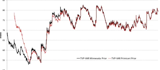
So far we have shown that the TVP-VAR index provides a more accurate depiction of the developments that affect the behavior of financial markets over time than the RW-VAR index. Next, we check whether the time series behavior of the connectedness index is due to the choice of the Bayesian TVP-VAR model we estimate, namely, the Minnesota prior. As an alternative to the TVP-VAR model with Minnesota Prior, we estimate the TVP-VAR model with the prior settings used in Primiceri (2005). This “Primiceri Prior” uses a certain amount of initial observations as the training sample. In our case, we set the training sample to 250 daily observations.
(TVP-VAR Primiceri for short) is presented in Figure 4 along with the one with Minnesota Prior. 50 55 60 65 70 75 80 85 6.04 12.04 6.05 12.05 6.06 12.06 6.07 12.07 6.08 12.08 6.09 12.09 6.10 12.10 6.11 12.11 6.12 12.12 6.13 12.13 6.14 12.14 6.15 12.15 6.16 In de x
TVP-‐VAR Minnesota Prior TVP-‐VAR Primiceri Prior
Figure 4: Total Connectedness: TVP-VAR Model with Primiceri Prior vs Minnesota Prior
For an overwhelming portion of the sample period, TVP-VAR model with Primiceri Prior based (VAR Primiceri) index follows a very similar path to that of our TVP-VAR index based on TVP-TVP-VAR model with Minnesota Prior. Despite a training sample of 250 days, TVP-VAR Primiceri index behaves quite differently in the first one-and-a-half years, namely from December 2004 to May 2006. For example, when the TVP-VAR index jumps close to 5 percentage points in December 2004 and June 2005 in response to the Great Indian Ocean Tsunami and Fed’s unexpected rate increase, respectively, the index based on TVP-VAR model with Primiceri prior does not respond to these news. However, the Primiceri-prior based index converges rapidly to the Minnesota-prior based index by May 2006. Afterwards, from May 2006 to the end-2008 the two indices behave quite close, with a maximum of one percentage point difference. After the end of 2008, the two indices behave almost identically.
6
Predictive
Performance
of
the
Connectedness
Index
So far we have compared the behavior of TVP-VAR and RW-VAR indices in sample. However, such a comparison is not sufficient in order to make claims about the usefulness of one index over the other. Systemic risk measures cannot be deemed useful if they
don’t provide predictive information on important systemic events. For that reason, in this section we focus on the performance of the two indices in predicting systemic events that had major impact in the U.S. and European financial markets.
6.1
Logit Analysis
There are no official statistics that one can use to identify systemic events. As a result,
researchers need to define systemic events using market-wide information. After
choosing an approach to identify systemic events, we can then go ahead and evaluate
the predictive performance of TVP-VAR and RW-VAR indices. Here we follow the
methodology proposed by Arsov et al. (2013) to identify systemic events. We define a systemic event as a day on which more than twenty-five percent of the US and
European financial institution stocks experience extreme loss. More specifically, we
construct a Systemic Event (SE) index, which indicates the fraction of banks
experiencing a return worse than 5th (left tail) percentile of its return distribution.
Then, the days on which SE exceeds 25 percent are labelled as systemic events.
After constructing the index, we investigate the relative performance of the two alternative connectedness indices in predicting future systemic events. To achieve this, we construct the following logit model.
PSE =P rob(SEt >0.25) =
1
1 +e−(β0+β1SEt−i+β2log(DY CI)t−i) (11)
where SE denotes the proportion of banks that experienced stock returns worse than the 5th percentile of its return distribution and DYCI is used as a measure of systemic risk. We use daily data to estimate Equation 11. In order to see the predictive power of the
index over time we estimate our logit model for different lags(i’s) from 1 to 50 days.
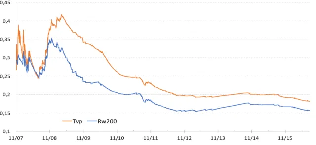
In Figure 5 we plot the McFadden R2 for predicting systemic events one-day ahead.
R2’s are plotted starting from November 2007, because before November 2007 there were
very few days on which systemic events as we defined here occurred.
Mc FaddenR2’s for both TVP-VAR and RW-VAR indices are higher during the global
financial crisis, from the last quarter of 2007 through 2009. When we compare the two
goodness of fit measures, the higher McFadden R2 for the TVP-VAR index compared
to that of the RW-VAR index is visible for the whole sample period. Especially, during the last quarter of 2007 and after the outburst of the global financial crisis (in the last
quarter of 2008 and throughout 2009 and 2010), McFadden R2 for TVP-VAR index is
5-10 percentage points higher than that of RW-VAR index. Out of 2235 observations for which the one-day ahead logit estimation is undertaken, there are only 40 observations
Figure 5: Extreme Event Predictive Performance (Logit; One-day Ahead ): TVP vs RW
for which the R2 for the TVP-VAR index is less than theR2 for the RW-VAR index.
Despite this evidence from the one-day ahead prediction exercise, it is too early to conclude that the TVP-VAR model outperforms the RW-VAR model based in predicting the future occurrence of the extreme events. To make sure what we observe in one-day ahead prediction performance also holds for longer time intervals, we compare the prediction performance of the two indices at 1-, 5-, 10-, 20- and 50-day ahead forecasting exercise.
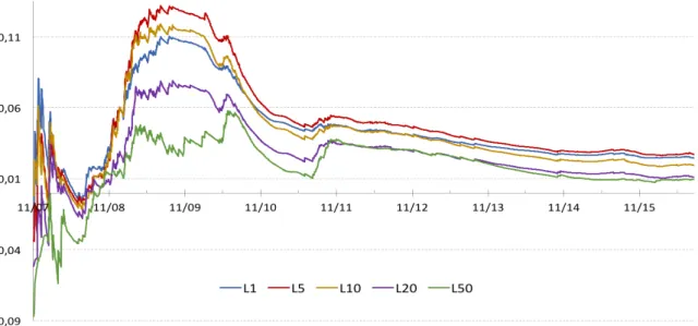
In Figure 6 we plot the difference between McFadden R2’s of logit models with
TVP-VAR and RW-TVP-VAR indices, respectively. Similar to the case of one-day ahead prediction, for the majority of lags and for subperiods, TVP-VAR index performs better than RW-VAR index in forecasting future extreme events. In general the difference between the goodness of fit measures fluctuate between 1 and 5 percentage points. During the early phase of the global financial crisis, logit model with the TVP-VAR index outperformed the model with RW-VAR index, but from April to July 2008, when markets were mostly in
a calm state, the McFaddenR2 difference declined and moved into the negative territory
for a brief period. Starting in August 2008 and in the most critical stage of the global financial crisis, the model with TVP-VAR index started to perform better than the one with RW-VAR index. By the end of 2008, the difference between the models reached 5 percentage points and moved up further and stayed high between 6 and 11 percentage points for a while. The difference between the two models’ forecast performance started to decline only after the Greek debt crisis of May 2010. By the end of 2010, the difference in forecasting performance declined to the 1-6 percentage point range and continued to stay in that range until the end of the sample in July 2016..
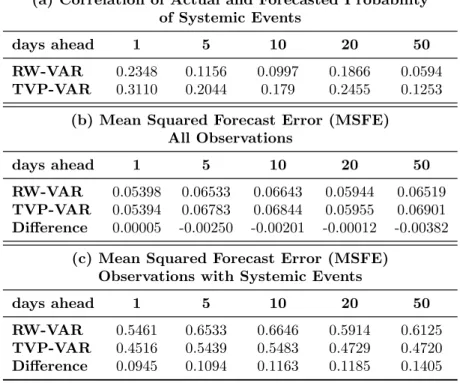
Figure 6: TVP - RW Difference in one- to 50-days ahead Predictive Performance One way of gauging the relative forecast performance of several models is to compare the respective correlation coefficients between the model forecasts and actual observations of the variable that is forecasted. In Table 4(a) we report the correlation coefficients between the actual and forecasts of the dependent variable, namely, the probability of
a systemic event (PSE) taking place. Again the logit model with the TVP-VAR index
outperforms the logit model with the RW-VAR index being used as the explanatory variable. Compared to the model with the RW-VAR index, the forecasts of the logit model with the TVP-VAR index have higher correlation with the actual observations of
PSE, the probability of the occurrence of a systemic event. The difference between the
correlation coefficients range from 6.5 and 9 percentage points for the forecast horizons we considered.
Finally, we compare the forecasting performance of the two logit models by focusing on their out-of-sample mean squared forecast error (MSFE) measures over the full sample. We report the MSFE of both models over the 1-, 5-, 10-, 20- and 50-day forecast horizons in Table 4(b). This is the only case where the difference between the two models is very little. If there is any difference, MSFEs indicate that it is in favor of the logit model including the RW-VAR index. However, when we focus on the days when a systemic
event occurred (that is when PSE = 1) then the MSFE measure overwhelmingly favours
the model with the TVP-VAR index over the one with the RW-VAR index. This indicates that the logit model with the TVP-VAR index is better in forecasting systemic events than the model with the RW-VAR index. Having better forecast performance over the observations with systemic events is quite a desirable property. It is also consistent with the results we reported above.
Table 4: Forecasting Systemic Events – RW-VAR vs TVP-VAR
(a) Correlation of Actual and Forecasted Probability of Systemic Events
days ahead 1 5 10 20 50
RW-VAR 0.2348 0.1156 0.0997 0.1866 0.0594
TVP-VAR 0.3110 0.2044 0.179 0.2455 0.1253
(b) Mean Squared Forecast Error (MSFE) All Observations
days ahead 1 5 10 20 50
RW-VAR 0.05398 0.06533 0.06643 0.05944 0.06519
TVP-VAR 0.05394 0.06783 0.06844 0.05955 0.06901
Difference 0.00005 -0.00250 -0.00201 -0.00012 -0.00382
(c) Mean Squared Forecast Error (MSFE) Observations with Systemic Events
days ahead 1 5 10 20 50
RW-VAR 0.5461 0.6533 0.6646 0.5914 0.6125
TVP-VAR 0.4516 0.5439 0.5483 0.4729 0.4720
Difference 0.0945 0.1094 0.1163 0.1185 0.1405
7
Conclusion
In this paper, we estimate a large TVP-VAR model of daily stock return volatilities for 35 U.S. and European financial institutions from January 2005 to July 2016 to derive Diebold-Yilmaz connectedness index measures. Unlike the dynamic total connectedness index obtained from the rolling-windows estimation of the VAR model, the TVP-VAR based connectedness index does not display excessive persistence. It declines gradually as the impact of the volatility shock on stock return volatilities disappeares. The rolling-window based connectedness index, on the other hand, stays high as long as the data pertaining to the crisis moment is kept within the rolling-sample window.
As the TVP-VAR model connectedness index does not suffer from the excessive persistence problem, it displays more pronounced jumps during major crisis moments, better capturing the increased tension in financial markets. As it may have already incorporated the impact of previous crisis moments, the rolling-windows based connectedness index jumps little during important crisis moments. For example, the TVP-VAR model based connectedness index went up 30 percentage points in four consecutive steps from the beginning of the U.S. sub-prime mortgage crisis in early March 2007 to January 2008, when the FOMC of Federal Reserve had to meet twice in a month to lower the interest rates by 125 bp in response to the increased pressure in
financial markets. Over the same period, the rolling-window based index, however, increased around 10 percentage points in two significant jumps. In the paper, we argued that the difference between the two indices is clearly visible throghout the 2004-2016 period.
Once we establish the difference between the two series, we then make sure that our results are robust to the choice of Bayesian VAR model. The index obtained from the TVP-VAR model with Primiceri prior deviates from the TVP-VAR model with Minnesota prior only during the first 18 months, from the end of 2004 to May 2006. From June 2006 onwards the two models produce connectedness indices that are closely syncronized.
Finally, we undertake a careful comparison of the performance of the two indices in predicting future systemic events. Using logit regression model we find out that the TVP-VAR index outperforms the RW-TVP-VAR index in predicting future systemic events, both in terms of standard measures of regression fit and in terms of forecasting.
Based on these findings, we conclude that the TVP-VAR model based dynamic connectedness index is a better candidate as a measure of systemic risk than the rolling-window based connectedness index.
References
Acharya, V.V., L. H. Pedersen, T. Philippon, and M. Richardson (2017), “Measuring
Systemic Risk,” Review of Financial Studies, 30, 2–47.
Adrian, T. and M. Brunnermeier (2016), “CoVaR,” American Economic Review, 106,
1705–1741.
Alizadeh, S., M.W. Brandt, and F.X. Diebold (2002), “Range-Based Estimation of
Stochastic Volatility Models,” Journal of Finance, 57, 1047–1091.
Arsov, I., E. Canetti, L. Kodres, and S. Mitra (2013), ““Near-Coincident” Indicators of Systemic Stress,” IMF Working Paper WP 13-115.
Cooley, T. (1971), Estimation in the presence of sequential parameter variation,
Unpublished PhD thesis, University of Pennsylvania.
Dangl, T. and M. Halling (2012), “Predictive Regressions with Time-varying
Coefficients,”Journal of Financial Economics, 106, 157–181.
Diebold, F.X. and K. Yilmaz (2012), “Better to Give than to Receive: Predictive
Measurement of Volatility Spillovers,”International Journal of Forecasting, 28, 57–66.
Diebold, F.X. and K. Yilmaz (2014), “On the Network Topology of Variance
Decompositions: Measuring the Connectedness of Financial Firms,” Journal of
Econometrics, 182, 119–134.
Diebold, F.X. and K. Yilmaz (2015), Financial and Macroeconomic Connectedness: A
Network Approach to Measurement and Monitoring, Oxford University Press.
Diebold, F.X. and K. Yilmaz (2016), “Trans-Atlantic Equity Volatility Connectedness:
U.S. and European Financial Institutions, 2004–2014,” Journal of Financial
Econometrics, 14, 81–127.
Engle, R.F. and B.T. Kelly (2012), “Dynamic Equicorrelation,”Journal of Business and
Economic Statistics, 30, 212–228.
Garman, M. B. and M. J. Klass (1980), “On the Estimation of Security Price Volatilities
From Historical Data,” Journal of Business, 53, 67–78.
Koop, G. and D. Korobilis (2013), “Large Time-Varying Parameter VARs,” Journal of
Koop, G., M.H. Pesaran, and S.M. Potter (1996), “Impulse Response Analysis in
Nonlinear Multivariate Models,” Journal of Econometrics, 74, 119–147.
Pesaran, H.H. and Y. Shin (1998), “Generalized Impulse Response Analysis in Linear
Multivariate Models,”Economics Letters, 58, 17–29.
Prado, R. and M. West (2010), Time Series Modeling, Computation, and Inference,
Chapman & Hall/CRC, New York.
Primiceri, G.E. (2005), “Time Varying Structural Vector Autoregressions and Monetary
Policy,”Review of Economic Studies, 72, 821–852.
Shumway, R.H. and D.S. Stoffer (1982), “An Approach to Time Series Smoothing and
Forecasting using the EM Algorithm,”Journal of Time Series Analysis, 2, 253 – 264.
Sims, C. (1989), “A Nine Variable Probabilistic Macroeconomic Forecasting Model,” Federal Reserve Bank of Minneapolis Discussion Paper No. 14.
Uhlig, H. (1994), “What Macroeconomists Should Know About Unit Roots,”
Econometric Theory, 10, 645–671.
Uhlig, H. (1997), “Bayesian Vector Autoregressions with Stochastic Volatility,”
Econometrica, 65, 59–73.
Walker, G. R. (2005), “Some Reflections on the Insurance Aspects of Tsunami Damage,”
http://www.aees.org.au/wp-content/uploads/2013/11/05-Walker.pdf,
Australian Earthquake Engineering Society.
West, M. and J. Harrison (1997), Bayesian forecasting and dynamic models, Springer
A
Technical Appendix
A.1
Sequential Bayesian inference for TVP-VARs
The VAR model we examine can be cast in the following state-space form
yt = xtβt+εt βt = βt−1+ηt wherext=I⊗ 1, yt0−1, ..., yt0−p,βt= A00, vec(A1) 0 , ..., vec(Ap) 00 andεt∼N(0,Σt) and ηt∼N(0,Ωt).
The initial condition for this model is defined by
β0 ∼ N(m0, C0)
Σ0 ∼ iW(S0, n0)
and the timet priors are
βt|Dt−1 ∼ N mt|t−1, Ct|t−1
Σt|Dt−1 ∼ iW St|t−1, nt|t−1
where mt|t−1 =mt−1, Ct|t−1 = 1λCt−1, St|t−1 =St−1, and nt|t−1 =δnt−1. Here λ and δ are
decay factors where λ, δ∈(0,1].
Given these priors, the time t posteriors take the form
• Posterior of Σt|t Σt|Dt ∼iW(St, nt) where nt = δnt−1 + 1 and St|t = (1−at)St−1|t−1 +at h St1−/21|t−1Qt−−11/2(εtε0t)Q −1/2 t−1 S 1/2 t−1|t−1 i , with at = n−t1 and
Qt−1 = Σt−1 + Ht−1Pt−1|t−1Ht0−1. In this formulation, εt is replaced with the
one-step ahead prediction error eεt|t−1 =yt−mt|t−1xt.
• Posterior of βt|t βt|Σt,Dt ∼N(mt, Ct) where mt =mt|t−1+Ct|t−1xtVt−1εetand Ct =Ct|t−1−Ct|t−1x 0 tV −1 t xtCt|t−1, with εet= yt−xtmt|t−1 the prediction error and Vt =xtCt|t−1x0t+ Σt its covariance matrix.
We allow the decay and forgetting factors to also over time using simple updating formulae: λt = λ+ (1−λ)×exp −0.5×bε0t−1Σb−t−11εbt−1 , (A.1)
δi,t = δ+ (1−δ)×exp (−0.5×kurt(bεt−22:t−1)), (A.2)
where Σbt−1 is the time t−1 estimate of the covariance matrix and kurt
b
Ei,t−12:t−1
is
the kurtosis of the VAR prediction error, evaluated over the past month. λ and κ put
bounds on the minimum values of the forgetting and decay factors. We set λ= 0.98 and
κ = 0.94 which, in the context of daily data, allow for the possibility of a fairly large