Randomness In Tree Ensemble Methods

University of Montana University of Montana

ScholarWorks at University of Montana

ScholarWorks at University of Montana

Graduate Student Theses, Dissertations, &

Professional Papers Graduate School

2009

Randomness In Tree Ensemble Methods

Randomness In Tree Ensemble Methods

The University of Montana

Follow this and additional works at: https://scholarworks.umt.edu/etd

Let us know how access to this document benefits you.

Recommended Citation

Elias, Joran, "Randomness In Tree Ensemble Methods" (2009). Graduate Student Theses, Dissertations, & Professional Papers. 795.

https://scholarworks.umt.edu/etd/795

This Dissertation is brought to you for free and open access by the Graduate School at ScholarWorks at University of Montana. It has been accepted for inclusion in Graduate Student Theses, Dissertations, & Professional Papers by an authorized administrator of ScholarWorks at University of Montana. For more information, please contact

RANDOMNESS IN TREE ENSEMBLE METHODS

by

Joran Elias

B.A. Dartmouth College, USA 2001

M.A. University of Montana-Missoula, USA 2004

presented in partial fulfillment of the requirements

for the degree of

Doctor of Philosophy

The University of Montana

May 2009

Approved by:

Dr. Perry Brown Graduate School Dr. Brian Steele, Chair

Mathematical Sciences Dr. Dave Patterson Mathematical Sciences Dr. Jon Graham Mathematical Sciences Dr. Soloman Harrar Mathematical Sciences Dr. Jesse Johnson Computer Science

Elias, Joran M. Ph.D., May 2009 Mathematics

Randomness in Tree Ensemble Methods

Committee Chair: Brian Steele, Ph.D.

Tree ensembles have proven to be a popular and powerful tool for predictive modeling tasks. The theory behind several of these methods (e.g. boosting) has received considerable attention. However, other tree ensemble techniques (e.g. bagging, random forests) have attracted limited theoretical treatment. Specifically, it has remained somewhat unclear as to why the simple act of randomizing the tree growing algorithm should lead to such dramatic improvements in performance. It has been suggested that a specific type of tree ensemble acts by forming a locally adaptive distance metric [Lin and Jeon, 2006]. We generalize this claim to include all tree ensembles methods and argue that this insight can help to explain the exceptional performance of tree ensemble methods. Finally, we illustrate the use of tree ensemble methods for an ecological niche modeling example involving the presence of malaria vectors in Africa.

Acknowledgements

I am grateful for the support from my advisor, Dr. Brian Steele, as well as for the many helpful comments and suggestions from my entire committee: Dr. Dave Patterson, Dr. Jon Graham, Dr. Solomon Harrar and Dr. Jesse Johnson. Finally, I am very thankful for the assistance I have received from the Department of Mathematical Sciences and the Montana-Ecology of Infectious Disease in the pursuit of my degree.

Contents

Abstract ii

Acknowledgements iii

List of Tables vii

List of Figures viii

1 Tree Ensemble Methods 1

1.1 Introduction . . . 1

1.2 Statistical Learning . . . 2

1.3 Decision Trees . . . 3

1.4 Tree Ensembles . . . 4

1.4.1 Theoretical justifications for tree ensembles . . . 6

1.5 A Look Ahead . . . 11

2 Metrics 13

2.1 Introduction . . . 13

2.2 Kernel Methods . . . 14

2.2.1 Introduction . . . 14

2.2.2 Optimal metrics . . . 15

2.3 Tree Ensembles as Kernel Method . . . 18

2.3.1 Introduction . . . 18

2.3.2 Partition Based Metrics . . . 19

2.3.3 Tree Ensembles as Kernel Methods . . . 22

2.3.4 d1 is Optimal for Kernel Methods Generally . . . 28

2.3.5 Connection to Optimal Metric . . . 29

2.4 A Look Ahead . . . 30

3 Variable Randomness in Stump Ensembles 32 3.1 Introduction . . . 32

3.2 Stump Ensembles . . . 33

3.3 Completely Random Stump Ensembles . . . 34

3.4 Variable Randomness Stump Ensembles . . . 36

3.5 Conclusion . . . 40

4 Local Models Using Tree Ensemble Weights 41 4.1 Introduction . . . 41

4.2 Fitting Local Models . . . 42

4.3 Numerical Study . . . 44

4.3.1 Results . . . 45

4.4 Local Models As Visualization Tool . . . 46

4.4.1 Local Model . . . 51

5 Case Study: Prediction of Malaria Presence from Environmental and Cli-matic Data 57 5.1 Introduction . . . 57 5.2 Data . . . 58 5.3 Random Forests . . . 60 5.4 Analysis . . . 61 5.5 Conclusion . . . 71 Bibliography 74 vi

List of Tables

1.1 Values for s,ρ¯, upper bound from (1.1) and error rates for PERT. Entries in parentheses are values for single trees (CART). . . 11

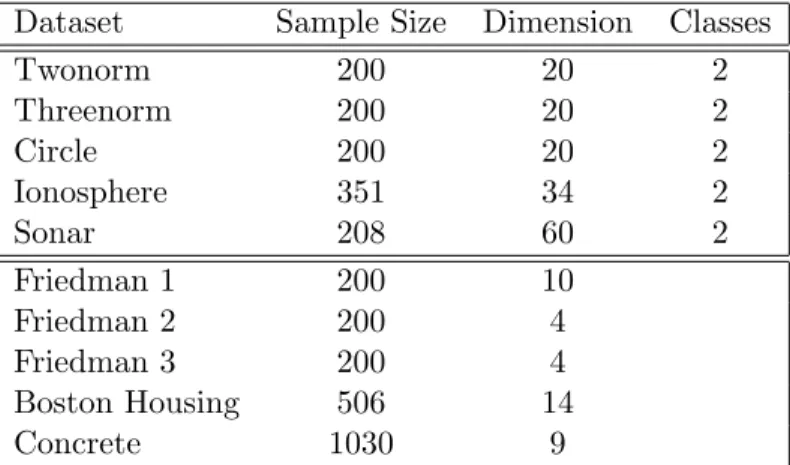
4.1 Dataset summaries. Twonorm, Threenorm, Circle and Friedman 1, 2 and 3 are the simulated data sets, the remaining are real data sets. . . 45

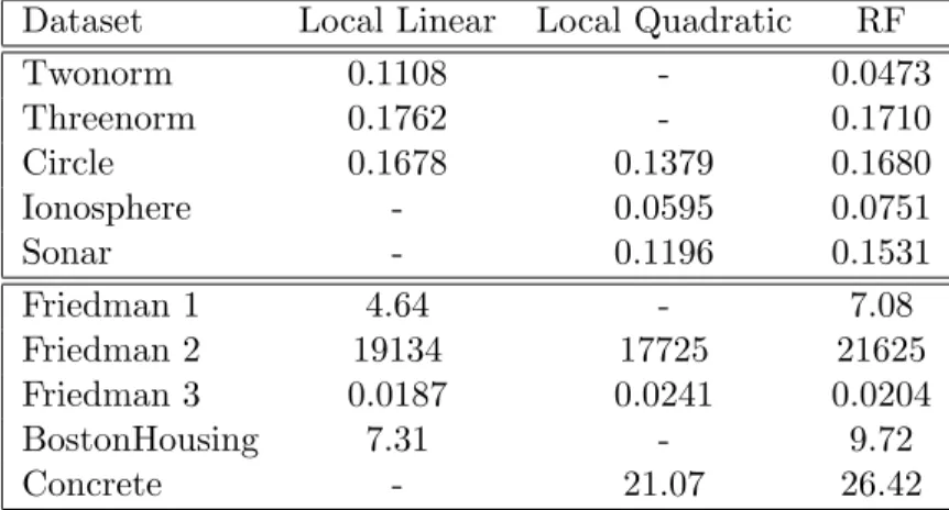
4.2 Mean out-of-bag error rates for random forests (RF) using its default settings and weighted linear/quadratic models using weights derived from the RF model. 46

5.1 Environmental parameters used in niche modeling. . . 59

5.2 Confusion matrix for malaria random forest niche model. The overall out-of-bag error rate was 0.039. (Rows are true values, columns are prediction by the RF model.) . . . 61

5.3 Logistic regression coefficients of best model resulting from backwards stepwise selection using AIC. . . 72

5.4 Logistic regression coefficients of best model resulting from manual backwards stepwise selection followed by forward addition of quadratic terms. . . 73

List of Figures

3.1 Training set (n= 500) used to construct stump ensembles. . . 38

3.2 Contour plots of Q(z0,z). Each panel is labeled according to the value of σ used in the ensemble. The point z0 is indicated as the black dot in the lower right of each panel. . . 39

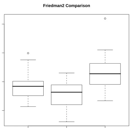
4.1 Boxplots of errors for simulation on the Friedman 2 dataset. . . 47

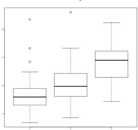
4.2 Boxplots of errors for simluation on the Friedman 3 dataset. . . 48

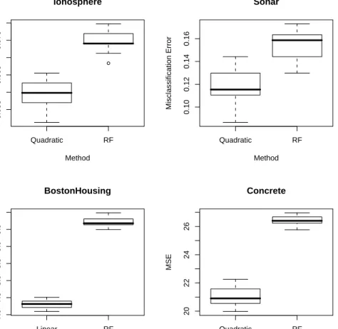
4.3 Boxplots of errors for the real data sets. . . 49

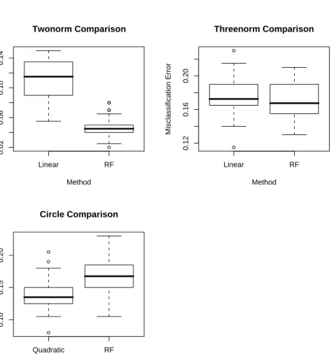
4.4 Boxplots of the errors for the simulated data sets. . . 50

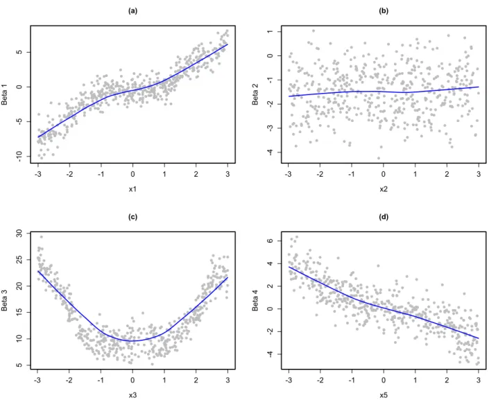
4.5 Plots of coefficients from local linear models versus variable values. . . 53

4.6 Plot of coefficients from local linear models versus variable values. . . 54

4.7 Scatterplots (with loess smooths in blue) of each coefficient with respect to their corresponding variable. . . 56

5.1 Variable importance plot for malaria vector niche model. . . 62

5.2 Partial dependence plot of altitude (in meters) on the log odds of malaria vector presence. . . 63

5.3 Partial dependence plot of precipitation of the wettest month (units unknown) on the log odds of malaria vector presence. . . 64

5.4 Partial dependence plot of precipitation of the wettest quarter (units unknown) on the log odds of malaria vector presence. . . 65

5.5 Partial dependence plot of landcover type (categories unknown) on the log odds of malaria vector presence. While the landcover classes associated with these categories is unknown, one might surmise that landcover 12 corresponds to something analogous to “desert”. . . 66

5.6 Partial dependence plot of the minimum temperature of the coldest month (units unknown) on the log odds of malaria vector presence. . . 67

5.7 Estimated coefficient versus Altitude for the locally linear model. . . 68

5.8 Estimated coefficient versus Precipitation of the Wettest Month for the locally linear model. . . 69

Chapter 1

Tree Ensemble Methods

1.1

Introduction

Tree ensembles1 (bagging, random forests, etc.) have proven to be one of the most successful

techniques in statistical learning. However, the theoretical understanding of tree ensembles

has lagged behind the empirical evidence for their success. The result has been a diverse array

of tree ensemble methods that perform very similarly to each other.

We will briefly review decision trees and tree ensemble methods, describe some of the different

tree ensemble methods and review some recent attempts at theoretical explanations for their

success. We conclude by suggesting that the motivation driving the creation of new tree

ensemble techniques is unsatisfactory and by offering a promising alternative.

1_{By this we mean non-adaptive tree ensembles, so we are excluding methods like boosting [15, 28] and arcing}

[3] that have received more complete theoretical treatments.

1.2. STATISTICAL LEARNING 2

1.2

Statistical Learning

In statistical learning we are presented with a data sample, or training set, (yi,xi) for i =

1, . . . , nwhere (Y,X) arise from some joint distributionfY,X(y,x). The valuesx= (x1, . . . , xp)

are referred to as feature vectors or covariates. LetX andYdenote the domains of the random

variables X and Y respectively. The goal is as follows: given some independently observed

test point x0, accurately predict the valuey0. (There are many other aspects to modeling, of

course, but here we will focus on predictive accuracy.)

This framework is divided further based on the nature of the values of y. When y is a continuous random variable, y∈_R, then we have a regression problem. Wheny is a discrete random variable taking the unordered values y ∈ {1, . . . , G}, then it is called a classification

problem. In either case, we model the conditional distribution of y given x: E[y|X=x] for regression and Pr[y =g|X=x] = Pr[g|X=x] for classification.

A statistical learner is a function f : X → Y that is intended to serve as an estimate of either E[y|X=x] or Pr[g|X=x]. Let L(ˆy, y) denote a loss function that measures the dis-crepancy between our function’s predictions and reality. This might be squared error loss or

misclassification rate. The apparent or empirical error is the average error over our training

sample: 1 n n X i=1 L(ˆyi, yi)

The expected prediction error, orgeneralization error is the expected loss over the distribution

of (Y,X): EY,XL(ˆy, y). The empirical loss is typically a biased estimate of the generalization

error and so various methods have been developed for obtaining more accurate estimates (for

1.3. DECISION TREES 3

1.3

Decision Trees

A decision tree is a piece-wise constant function, f(x), on the feature space X. Let Π =

{R1, . . . , Rm} be a partitioning of X. A decision tree is constant on each region Ri ∈ Π.

Specifically, if x0∈Ri, and Ri also contains the training points{(y1,x1), . . . ,(y`,x`)}then

f(x0) =      1 ` P` iyi y∈R arg maxP` iI(yi=g) y∈ {1,2, . . . , G}

where I denotes the indicator function. That is, f simply predicts the average response (or majority class) in each region Ri ∈Π. When y is discrete we have written f as returning a

class label, but we can easily modify f to estimate the class probabilities by the proportion of training observations of each class in a region.

Clearly, the challenge is in constructing an optimal partition Π. Searching for an optimal

partition is generally a difficult combinatorial problem so we will simplify things considerably.

This is done via a greedy algorithm and by restricting ourselves to a small class of partitions:

those using only binary splits of the form: xi ≤c.

This greedy algorithm is often called recursive binary partitioning, which leads to the

char-acteristic “tree” structure. We begin with all of the training data in the root node and we

perform an exhaustive search for the binary split of the form xi ≤ c that minimizes a loss

function L(ˆy, y). All of the training observations for which xi ≤c constitute the left

daugh-ter node (or child node) and the training observations for which xi > c constitute the right

daughter node. We then repeat our search for a split on each daughter node. The process

continues recursively until there is only one training observation in each node. These nodes

1.4. TREE ENSEMBLES 4

A partitioning with only one training observation in each terminal node is typically not

op-timal. Specifically, its generalization error will often be very high. Many methods have been

developed to prune a maximally grown decision tree (cf. [4]). We will not address these

methods here, as they are fairly involved and are not typically used in tree ensemble methods.

Instead we will simply refer to trees that are “grown” until there are a maximum number

of training observations in each terminal node. When this number is small we will split our

training data many times and get a “large” tree, while when this number is large we will split

our training data only a few times and get a “small” tree. This is called a stopping criteria:

we stop splitting nodes when they contain ≤ktraining observations.

1.4

Tree Ensembles

A tree ensemble is simply a statistical learner that is defined to be the average (or majority

vote, in the classification case) over a collection of trees, f1, . . . , fB.

The first tree ensemble method was bootstrap aggregation, orbagging [2]. Suppose we drawB

bootstrap samples from the training set and fit a decision tree using each bootstrap replicate:

f₁∗, . . . , f_B∗. Each bootstrap sample will result in a slightly different partitioning and hence a slightly different decision tree. Then the bagged decision tree is

fe(x) = 1 B B X b=1 f_b∗(x) for a continuous response y, and

fe(x) = arg max g B X b=1 I(f_b∗(x) =g)

1.4. TREE ENSEMBLES 5

when y is categorical. Hence when y is continuous we average the predictions f_b∗(x) and when y is categorical we take the majority vote among the f_b∗(x). Again, this expression is easily modified to estimate the class probabilities directly. Breiman [2] demonstrated that

this simple procedure significantly outperforms single pruned decision trees.

The success of bagging spurred the development of other methods that employ increasing

amounts of randomization in the creation of the individual decision trees. Breiman [5]

intro-duced Random Forests (RFs) based on a technique developed by Amit and Geman [1]. In

RFs, trees are built on bootstrap samples of the data, as in bagging. However, at each node

of each tree, the algorithm only searches over a randomly selected subset of the covariates

for the best split. Breiman also discussed randomizing the procedure further by searching for

splits over random linear combinations of covariates (RF-RC): at each node selectLvariables and create F linear combinations of these L variables using coefficients generated randomly on the interval [−1,1].

Ho [20] suggested the random subspace method (RS), which is essentially identical to RFs

but omits the bootstrap resampling. Cutler and Zhao [10] introduced perfect random tree

ensembles (PERT) for classification tasks. In PERT, trees are constructed as follows: at

each node two data points xi = (xi1, . . . , xip), xj = (xj1, . . . , xjp) are selected at random

until they belong to different classes (if this is not possible, all values in this node are in

the same class, and the node is terminal); randomly choose a feature, k, and split the data at αxik + (1 −α)xjk where α ∼ U(0,1). Cutler and Zhao note that this procedure can

be performed with or without bootstrapping. They observe that PERT achieves accuracies

similar (or better) than AdaBoost, RF, and RF-RC with running times that are considerably

faster.

Geurts et al. [17] introduced extremely randomized trees (ERT). Here, at each node a random

subset ofLvariables is selected, as in RFs. However, ERTs then select a split point completely at random on each of these Lvariables and split the node on the best of theseL splits. This

1.4. TREE ENSEMBLES 6

procedure is essentially identical to that suggested by Lin and Jeon [22], although they call it

random point selection (RPS). They also note that this procedure can easily be incorporated

into RF-RC: a split is randomly chosen on each linear combination and the best of these

is selected to split the data. Lin and Jeon observe that this procedure maintains very high

accuracies while running much faster than traditional bagging or RF procedures that search

over all possible splits on each covariate.

Several authors have examined completely random trees (CRT) [13, 14, 23], where each split is

chosen randomly, without evaluating any of the commonly used improvement criteria such as

gini index, mean squared error (MSE) or variance reduction. Surprisingly, even this amount

of randomness seems to work very well, although it appears to perform poorly when a large

number of irrelevant features are present [24]. This problem can be ameliorated by varying

the probability that one chooses a split randomly or according to some improvement criteria

at each node [24].

In general, each author recommends growing large trees (i.e. a small number of training

observations in each terminal node), frequently the largest trees possible, although Lin and

Jeon [22] suggest that this may not always be optimal. Typically what is recommended is

growing trees until there are between 1 and 5 observations per terminal node, depending on

the particular algorithm and whether the problem is one of classification or regression.

1.4.1 Theoretical justifications for tree ensembles

We begin by reviewing Breiman’s [2] justification for bagging. Suppose that y is continuous (a similar argument exists for when y is discrete, which we omit) and that we can collect multiple independent training setsT from a distribution and fit a learner (i.e. a decision tree)

on each set, f(x,T). Then the aggregated learner is defined to be the expected prediction over all possible training sets,

1.4. TREE ENSEMBLES 7

fA(x) =ET(f(x,T)).

Let (y0,x0) be an independent test point. Using squared-error loss we have,

ET(y0−f(x0,T))2 =y02−2y0ETf(x0,T) +ETf2(x0,T)

Substituting ETf(x0,T) =fA(x0) and applying the inequality EZ2 ≥(EZ)2 yields

ET(y0−f(x0))2 ≥(y0−fA(x0))2.

Integrating over (Y,X) on both sides shows that the mean squared error of the aggregated learner is never greater than the mean squared error of a learner fit to a single training set.

Breiman asserts that how much improvement we see depends on how unequal the two sides

of

(ETf(x0,T))2 ≤ETf2(x0,T)

are. In essence, the more variablef(x,T) is with each individual training setT, the greater the advantage of the aggregated predictor fA. Hence Breiman claims the advantage of bagging

is to reduce variance, and will be particularly effective for learners that are in some sense

“unstable”. By unstable, Breiman means that small perturbations in the training set T

produce large changes in the functionf(x,T).

Obviously, it is not possible to sample randomly with replacement from the distribution that

1.4. TREE ENSEMBLES 8

the empirical distribution placing mass 1/n at each training point in T. The hope is that sampling from the bootstrap distribution will be a good approximation to sampling from the

distribution that generated the actual data. As has been noted elsewhere [31], this is not

really a proof that bagging works so much as a justification for why it’s reasonable to try. It

is important to note that many of the subsequently developed tree ensemble methods omit

bootstrapping entirely and still perform very well. This strongly suggests that data resampling

is not a crucial element of the success of tree ensembles.

There have been other limited investigations of tree ensembles, mostly focusing on bagging.

Domingos [12] suggested from a Bayesian perspective that bagging “shifts the priors to a

more appropriate model space”. Buja and Stuetzle [7] examine bagging in the limited case of

U-statistics and find that bagging always increases bias and that the effect on variance and mean squared error (MSE) depend on the particularU-statistic and its distribution. Friedman and Hall [16] provide a heuristic argument that bagging can reduce variance, although their

argument applies only to smooth estimators, whereas trees are non-smooth (the function is

not continuous). Buja [8] also argues in a very general setting that bagged functionals are

always “smooth” even if the original functional is not. Buhlmann and Yu [6] argue that

bagging results in a smoother decision boundary which in turn reduces variance. Unlike most

other investigations, Buhlmann and Yu address bagged decision trees directly, although the

theoretical results become very technical and shed little light on the essential mechanism of tree

ensembles. Grandvalet [18] observed that bagged decision trees tend to equalize the influence

of each training point on the resulting learner. Few of the more randomized tree ensembles

have received much theoretical examination. Cutler and Zhao [10] observe that PERT fits a

“blockwise multilinear interpolating surface.” They note that this can be calculated exactly

using some extremely complicated recursive equations but that it is faster to use Monte Carlo

estimation.

Some more promising results have been achieved for RFs. Breiman [5] proved that RFs

1.4. TREE ENSEMBLES 9

RFs will not overfit the training data. He also derives an upper bound on the generalization

error for RFs for classification, which we review here.

Letf(x, θ) denote a learner in an ensemble corresponding to the random vectorθand assume that y is categorical. In the specific case of RFs, f(x, θ) is a single tree where θ denotes the bootstrap sample used and the variables selected at each node. We can think of θ as representing the randomness injected into the tree construction procedure. Hence different

realizations of the random vectorθwill yield slightly different trees. Define the margin function for a RF as

mr(x, y) =Pθ(f(x, θ) =y)−max

j6=y Pθ(f(x, θ) =j)

as the difference between the proportion of ensemble members making a correct prediction at

the point (x, y) and the proportion of ensemble members predicting the second most likely class. The margin function can be thought of as measuring the certainty of an ensemble’s

predictions. Define the strength of a set of classifiers as

s=EX,Ymr(x, y),

the expectation of the margin over all points (x, y). Note that−1≤mr(x, y), s≤1. To ease notation, let

ˆ

j(x, y) = arg max

j6=y Pθ(f(x, θ) =j)

denote the second most commonly predicted class at a point (x, y). Define the raw margin function as

1.4. TREE ENSEMBLES 10

rmg(θ,x, y) =I(f(x, θ) =y)− I(f(x, θ) = ˆj(x, y))

so that mr(x, y) is the expectation of rmg(θ,x, y) over the random vector θ. Let ρ(θ, θ1)

denote the correlation between rmg(θ,x, y) and rmg(θ1,x, y) where θ and θ1 are fixed and

the point (x, y) is allowed to vary. Finally, let ¯ρ denote the mean value of this correlation over all pairs of realizations of θ. Breiman proves that the generalization error for RFs, P E∗, is bounded by

P E∗≤ ρ¯(1−s

2₎

s2 (1.1)

The correlation ¯ρmeasures the extent to which the same training points are correctly classified by different trees. For example, if each tree correctly classifies the same subset of training

points, then ¯ρ= 1. A similar bound can be proven for the regression case, relating prediction error to the correlation between residuals and the overall strength of each tree.

Breiman concludes that the goal in constructing tree ensembles is to decrease the correlation

between trees while maintaining their overall strength. This conclusion has driven much of the

pursuit for random tree building procedures in order to reduce ¯ρ. Many (PERT, ERT, CRT etc.) are motivated by an attempt to make the individual trees as uncorrelated as possible.

However, this path has had several drawbacks:

ˆ The bound in (1.1) is likely to be loose. Indeed, in the unit square the median value of this upper bound is roughly 1.2. In [5] Breiman calculates estimates of ¯ρ and s for three data sets. For the sonar data the bound exceeds 1; for the satellite data the bound

is about 5 times higher than the actual accuracy achieved and it is fairly tight for the

1.5. A LOOK AHEAD 11

is in [10] using PERT and CART. The results are summarized in Table 1.1. Note that

the upper bound is always far higher than the best error rate achieved with PERT (and

is once greater than one). Also observe that in two cases the upper bound for single

CART trees is actuallylower than for PERT, even though their error rates are higher.

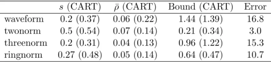
Table 1.1: Values for s,ρ¯, upper bound from (1.1) and error rates for PERT. Entries in parentheses are values for single trees (CART).

s (CART) ρ¯(CART) Bound (CART) Error waveform 0.2 (0.37) 0.06 (0.22) 1.44 (1.39) 16.8 twonorm 0.5 (0.54) 0.07 (0.14) 0.21 (0.34) 3.0 threenorm 0.2 (0.31) 0.04 (0.13) 0.96 (1.22) 15.3 ringnorm 0.27 (0.48) 0.05 (0.14) 0.64 (0.47) 10.7

ˆ Reducing ¯ρ has diminishing returns. The most extreme randomization exists in PERT and CRT and the correlations achieved by PERT are remarkably small (Table 1.1).

However, the improvements in accuracy over methods like bagging and RFs are relatively

modest.

ˆ This bound fails to account for the particular success of randomization in decision tree ensembles as opposed to other learners. In deriving this bound, f(x, θ) could refer to any base learner, including those known to receive little benefit from bagging (i.e. k

nearest neighbor). Why randomization techniques should be so successful with trees

but not with other learners is unclear.

1.5

A Look Ahead

We have given a short introduction to decision trees, tree ensembles and some of the

theoret-ical justifications for the success of these methods. Also, we have argued that the principal

theoretical justification has some serious shortcomings. In the following chapter, we will

1.5. A LOOK AHEAD 12

a connection between tree ensembles, weightedk-nearest neighbor methods and distance met-rics.

Chapter 2

Metrics

2.1

Introduction

In this chapter we will expand upon an observation by Lin and Jeon [22] to connect all

tree ensemble methods to weighted k-nearest neighbor, or kernel methods. We will discuss the concept of an optimal distance metric and see how this relates to the behavior of tree

ensembles in general. We begin with the following definitions.

Definition 2.1.1. A function d(x,y) is called a metric when it satisfies the following condi-tions, 1. d(x,y)≥0 2. d(x,y) =d(y,x) 3. d(x,y) = 0⇔x=y 4. d(x,y)≤d(x,z) +d(z,y). 13

2.2. KERNEL METHODS 14

Definition 2.1.2. A function d(x,y) is called a pseudometric when it satisfies conditions 1, 2 and 4 from Definition 2.1.1.

Clearly, every metric is a pseudometric, but not vice versa. However, any pseudometric d

gives rise to a genuine metric in the following manner. Define an equivalence relation between

the pointsx and yby

x∼y⇔d(x,y) = 0.

Then dis a metric on the resulting equivalence classes.

Definition 2.1.3. A kernel is a non-negative real valued function that satisfies the following

two conditions,

ˆ R∞

−∞K(u)du= 1

ˆ K(−u) =K(u).

We note here the important point that if K is a kernel, then so is Kλ(u) = λ−1K(λ−1u) for

λ >0.

2.2

Kernel Methods

2.2.1 Introduction

Kernel methods are a general statistical learning method that estimates the conditional

distri-bution ofy locally. The local nature of these methods are obtained via a kernel function that identifies training observations that are in some sense “close” to the test point at which we

2.2. KERNEL METHODS 15

would like to make a prediction. Almost any model for the conditional expectation ofycan be made “local” by introducing weights corresponding to a particular kernel function. Examples

include weighted versions of linear and non-linear parametric models. Here we consider only

the simplest form, a locally constant model, commonly called the Nadaraya-Watson estimator,

ˆ E(y|X=x0) = Pn i Kλ(x0,xi)yi Pn i Kλ(x0,xi)

stated here for the case thaty is continuous, where the kernel function acts by

Kλ(x0,x) =K d(x0,x) hλ(x0) (2.1)

where d is some distance metric and hλ is a scaling factor, commonly called the bandwidth.

The analogous version wheny is discrete is simply

c Pr(g|X=x0) = Pn i Kλ(x0,xi)I(yi=g) Pn i Kλ(x0,xi) .

Note that scaling byPn

i Kλ(x0,xi) is somewhat redundant, since this scaling factor could be

incorporated into the bandwidth functionhλ.

With the appropriate choice of hλ and K this definition includes the well known k-nearest

neighbor and weightedk nearest neighbor methods.

2.2.2 Optimal metrics

The notion of “closeness” that is embodied in a kernel is largely captured by the distance metric

used in 2.1. It is well known ink-nearest neighbor modeling that the choice of distance metric can dramatically affect performance. This has motivated the identification of an optimal

distance metric. The central result in this vein is by Cover and Hart [9], where they motivate

2.2. KERNEL METHODS 16

classification. We review this result here.

Let xnn denote the closest training point to the independent test point x0. The risk of a

1-nearest neighbor classifier is the probability that we misclassify x0. We will shorten our

notation slightly so that, for example, Pr(1|x0) = Pr(Y0 = 1|x0) and Pr(1|xnn) = Pr(Ynn =

1|xnn). They begin by substituting the asymptotic risk of the 1-NN rule with its upper bound

(see [29],[26] for a derivation of this bound):

r?(x0) = 2 Pr(1|x0) Pr(2|x0)

On the other hand, the finite sample risk is given by

r(x0,xnn) = Pr(1|x0) Pr(2|xnn) + Pr(2|x0) Pr(1|xnn) = Pr(1|x0) Pr(2|xnn) + Pr(1|x0)−Pr(1|x0) Pr(2|x0)−Pr(1|x0) + Pr(1|x0) Pr(2|x0) + Pr(2|x0) Pr(1|xnn) = Pr(1|x0) Pr(2|x0) + Pr(1|x0)−Pr(1|x0) Pr(2|x0)−Pr(1|x0) + Pr(1|x0) Pr(2|xnn) + Pr(2|x0) Pr(1|xnn) = Pr(1|x0) Pr(2|x0) + Pr(1|x0) [1−Pr(2|x0)]−Pr(1|x0) [1−Pr(2|xnn)] + Pr(2|x0) Pr(1|xnn) = Pr(1|x0) Pr(2|x0) + Pr(1|x0)2−Pr(1|x0) Pr(1|xnn) + Pr(2|x0) Pr(1|xnn) = 2 Pr(1|x0) Pr(2|x0) + Pr(1|x0)2−Pr(1|x0) Pr(1|xnn)− Pr(1|x0) Pr(2|x0) + Pr(2|x0) Pr(1|xnn) = 2 Pr(1|x0) Pr(2|x0) + [Pr(1|x0)−Pr(2|x0)]·[Pr(1|x0)−Pr(1|xnn)]

2.2. KERNEL METHODS 17

to choose a distance metric that minimizes the difference between the asymptotic and finite

sample risk of the 1-nearest neighbor model. The difference is simply

r(x0,xnn)−r?(x0) = [Pr(1|x0)−Pr(2|x0)]·[Pr(1|x0)−Pr(1|xnn)].

So for a fixed x0, minimizing this is equivalent to minimizing |Pr(1|x0) − Pr(1|xnn)| or

[Pr(1|x0)−Pr(1|xnn)]2. Hence, for two class classification, when using the 1-NN learner,

we should use as a distance metric the function

d1(x1,x2) =|Pr(1|x1)−Pr(1|x2)|. (2.2)

Arguing by analogy, there are several options for extending this metric to multi-class

classifi-cation (cf. [26]), among them

d1(x1,x2) = G X g=1 |Pr(g|x1)−Pr(g|x2)|, or d1(x1,x2) = G X g=1 Pr(g|x1)· |Pr(g|x1)−Pr(g|x2)|.

Similarly, the analogous version ofd1for a continuous response would bed1(x1,x2) =|E[y|x1]−

E[y|x2]|.

The first thing to note is that 2.2 is not, in fact, a metric. Specifically, we may have two points

x1 6=x2 where d1(x1,x2) = 0, so it fails condition (3) in Definition 2.1.1. Henced1 is in fact

a pseudometric, which can be converted to a true metric by considering equivalence classes

defined by those points where Pr(1|x1) = Pr(1|x2). Additionally, the usefulness of this metric

seems limited, since if weknew the conditional class probabilities, a simple application of Bayes

rule would yield the optimal classifier. Specifically, if we knew Pr(g|x0) forg= 1, . . . , G, then

2.3. TREE ENSEMBLES AS KERNEL METHOD 18

Intuitively, this metric is telling us that observations that lie on similarcontours of the

condi-tional expectation ofyshould be considered “close”. Note that this may or may not correspond to our intuitive notion of distance in the spaceX. Two points x1 and x2 might be very

dis-tant in terms of their Euclidean distance, but if the conditional expectation ofy at these two points is very close, then in some sense they are very “similar”. Several authors ([11], [19])

have used this result to motivate the development of local distance metrics, that create a

unique distance metric for each test pointx0 that accounts for the local characteristics of the

conditional distribution ofy. Usually, this is done through some form of feature weighting. For example, if near x0 the conditional distribution of y changes rapidly in the xi direction, but

remains relatively constant in thexj direction, then in the resulting metric thexi coordinate

will receive a large weight and xj a small weight.

2.3

Tree Ensembles as Kernel Method

2.3.1 Introduction

Here we will characterize all tree ensemble methods as kernel models. Specifically, the

pre-dictions from tree ensembles are weighted averages of the training data, and the weights are

based upon a distance metric created by the tree ensemble. This basic idea was first noticed

by Lin and Jeon [22]; we extend this notion to include all tree ensembles rather than just a

particular type of random forest model.

Next, we explain how the metric created by tree ensembles is related to the optimal 1-NN

metric d1 described above, and provide a general, heuristic argument that this type of metric

2.3. TREE ENSEMBLES AS KERNEL METHOD 19

2.3.2 Partition Based Metrics

Let Π1, . . . ,ΠB be a finite number of partitions on the space X, with Πi = {R1i, . . . , Rmi}.

Hence in each Πi, R`∩Rj = ∅ for all ` 6= j and S`R` = X. Let A(x1,x2,Π) denote the

event thatx1 andx2 lie in the same region of the partition Π. In other words, there exists an

R` ∈Π such thatx1,x2∈R`.

Further, let Q(x1,x2) be defined as

Q(x1,x2) = 1 B B X i=1 I(A(x1,x2,Πi))

and let d2(x1,x2) = 1−Q(x1,x2). So Q(x1,x2) is simply the proportion of times that x1

and x2 lie in the same region over all partitions Π1, . . . ,ΠB. First we prove that d2 is a

pseudometric.

Proposition 1. The function d2(x1,x2) = 1−Q(x1,x2) is a pseudometric.

Proof. First we observe that d2(x1,x2) ≥ 0 simply by construction. By the properties of a

partition and set inclusion, we have that the eventA(x1,x2,Π) occurs if and only if the event

A(x2,x1,Π) occurs, so we immediately have that d2(x1,x2) = d2(x2,x1). To demonstrate

thatd2 satisfies the triangle inequality, we must show that

d2(x1,x2)≤d2(x1,x3) +d2(x3,x2)

which is equivalent to showing that

1−Q(x1,x2)≤1−Q(x1,x3) + 1−Q(x3,x2)

or finally that

2.3. TREE ENSEMBLES AS KERNEL METHOD 20

The remaining part of the proof proceeds by induction on the number of partitions, B. First suppose there is only one partition, Π1. Then the functionQcan take only the values 1 or 0.

The only way the inequality could be violated is ifQ(x1,x2) = 0 butQ(x3,x2) =Q(x1,x3) =

1. But this would imply that there exists anR` ∈Π1 such that x3,x2 ∈R` and there exists

an Rj ∈Π1 such that x1,x3 ∈Rj. But by the properties of partitions, this would imply that

R` =Rj, and thatx1,x2∈Rj =R` which contradictsQ(x1,x2) = 0.

Now suppose that the inequality holds for B partitions, and let ΠB+1 be another partition.

To ease notation, define

a = B X i=1 I(A(x1,x3,Πi)) b = B X i=1 I(A(x3,x2,Πi)) c = B X i=1 I(A(x1,x2,Πi))

so thata, b, csimply count the number of times that each pair of points lies in the same region over the firstB partitions. Then by our induction hypothesis we have that

a B + b B ≤ 1 + c B, a+b ≤ B+c.

Now, when we add the partition ΠB+1, there are only three possibilities: (1) each of a, b, c

2.3. TREE ENSEMBLES AS KERNEL METHOD 21

unchanged, or (3) they all remain unchanged. In the first case we would have

a+ 1 B+ 1+ b+ 1 B+ 1 ≤ 1 + c+ 1 B+ 1 a+ 1 +b+ 1 ≤ B+ 1 +c+ 1 a+b ≤ B+c.

Similarly, if we assume that (without loss of generality) only ais increased by one we would have a+ 1 B+ 1+ b B+ 1 ≤ 1 + c B+ 1 a+ 1 +b ≤ B+ 1 +c a+b ≤ B+c

Finally, if none of a, b, care increased by one, we are left with

a+b≤B+ 1 +c

and so the expression holds in each case.

It is easy to note thatd2 may fail (3) from Definition 2.1.1; namely, two points x1 6=x2 may

lie in the same region in every partition Πi and hence would have d2(x1,x2) = 0. As noted

above, we can create a true metric from d2 simply by defining equivalence classes consisting

of those points whose distance is zero and allowing d2 to act on the equivalence classes.

2.3. TREE ENSEMBLES AS KERNEL METHOD 22

1.

Corollary 2.3.1. For any tree ensemble method the functiond2, defined as above, is a pseu-dometric (and hence there exists an associated metric), on the feature space X.

We emphasize that this corollary applies to any tree ensemble, regardless of the depth of the

trees, or the nature of their construction. All that is required is that each tree consists of a

partition of X.

2.3.3 Tree Ensembles as Kernel Methods

We begin by describing Lin and Jeon’s original observation in this vein, in which they

consid-ered a restricted class of random forest tree ensembles. Specifically, consider a tree ensemble

in which each tree is grown to maximal depth: each leaf of each tree contains only a single

training point.

This is slightly awkward in a classification setting, since if a node contains multiple training

points all from the same class (i.e. the node is pure) we would typically not continue to

split that node. So we must make the assumption that pure nodes with more than one

training observation will be split, albeit randomly. (How we split pure nodes is irrelevant

to the resulting ensemble, since the predictions will remain unchanged.) We can handle the

analogous situation for regression in the same manner.

As before, let Π1, . . . ,ΠB denote B trees (i.e. partitions of X) grown in this fashion on the

2.3. TREE ENSEMBLES AS KERNEL METHOD 23

simply a weighted average of the yi’s:

ˆ E(y|x0) = n X i=1 Q(xi,x0)yi ify is a continuous response (2.3) c Pr(g|x0) = n X i=1 Q(xi,x0)I(yi =g) if y is a discrete response (2.4)

where the function Q has the same meaning as in equation 2.3; namely the proportion of times that xi and x0 lie in the same region (terminal node) over all partitions (trees). In

addition, we see that these tree ensembles are creating a unique distance metric and then

fitting a distance weightedn-nearest neighbor model. In practice, many of the training points receive a weight of 0, so we might say that the ensemble is fitting a distance weightedk-nearest neighbor model, where k(and the metric!) is different for each test point x0.

Of course, in actual implementations of tree ensembles it is often the case that we do not

construct each tree such that every terminal node contains only a single training point. Hence,

we might ask what can be said about tree ensembles in general: what happens if we relax the

requirement that each terminal node contains only a single training point? The answer will

require a simple modification of our definition ofQ.

Let us assume again that we haveBpartitions (trees), Π1, . . . ,ΠBand a training set (yi,xi)ni=1.

We need not have used the training set to create the partitions (trees), Πi, but there must be

at least one training point in every region of every partition. Let Ri(xj) denote the region

in partition (tree) Πi that contains the point xj. Finally, let |Ri(xj)|denote the number of

training points contained in the regionRi(xj).

Suppose for the moment that y is continuous and consider a pointx0 not in the training set.

We can write the prediction made by the tree ensemble at the point x0 using the notation

2.3. TREE ENSEMBLES AS KERNEL METHOD 24 ˆ y0= 1 B B X i=1 |Ri(x0)|−1   X yj∈Ri(x0) yj  . (2.5)

So this is simply an average of averages; we average the mean of theyj’s in each node containing x0. If we rearrange the terms in this sum we find that the weight that each training value yj

receives in the final prediction is simply the sum of the |Ri(x0)|−1 over the yj, the reciprocal

of the number of training observations in each node containingyj.

We have used the notation z1,z2 to emphasize that they may not be points in the training

set. Then we can write equivalent expressions to Equations 2.3 and 2.4 by modifying our

definition ofQ. Specifically, we define Q? _as

Q?(z1,z2) = 1 B B X i=1 |Ri(z1)|−1I(A(z1,z2,Πi)). (2.6)

Note thatQ? includesQas a special case, when|Ri(zj)|= 1 for alli, j. Additionally, we note

that |Ri(zj)| only counts the training points contained in that region of a partition (tree).

With this modification, we can say that for any tree ensemble,

ˆ E(y|x0) = n X i=1 Q?(xi,x0)yi ify is a continuous response (2.7) c Pr(g|x0) = n X i=1 Q?(xi,x0)I(yi =g) if y is a discrete response (2.8)

There are some important differences betweenQ and Q?. First, our definition of Qrequired only a collection of partitions (trees) on the spaceX;Q?requires both a collection of partitions (trees)and a training set (yi,xi)ni=1. Additionally, we require that each region in each partition

contain at least one training point; there can be no “empty” regions. However, we again note

that the training points need not have been used to create the partitions (trees).

2.3. TREE ENSEMBLES AS KERNEL METHOD 25

pseudometric is also bounded between 0 and 1. However, when we allow more than one

training observation in each region (terminal node) of every partition (tree), the bounds on

Q? may be different. Specifically, if z1 and z2 never lie in the same region (terminal node),

thenQ?(z1,z2) = 0, so the lower bound is the same. However, suppose thatz1 andz2 always

lie in the same region (terminal node), but that one of those regions contains more than one

training point: |Ri(z1)|>1. ThenQ?(z1,z2)<1.

To make this observation more concrete, suppose that there are exactlyk >1 training observa-tions in each region (terminal node). Then ifz1 andz2 always lie in the same region (terminal

node) we have thatQ?(z1,z2) = 1/kso the function Q? is bounded 0≤Q?(z1,z2)≤1/k. In

general, there may be a different number of training points in each region of each partition,

so determining universal bounds on Q? is in practice unrealistic. However, we can observe that increasing the average number of observations per region (terminal node) will generally

cause the values Q?(xi,x0) in (2.8) to be more evenly distributed across the training points

xi. Conversely, decreasing the average number of observations per region (terminal node) will

cause the values Q?_(x

i,x0) to depend on only a handful of training points.

The fact that there may be different numbers of training points in each region of every partition

gives the impression that Q? is considerably more complex than Q. However, this is not necessarily the case. Assume, as above, that every region of each partition Π contains exactly

2.3. TREE ENSEMBLES AS KERNEL METHOD 26 Q?(z1,z2) = 1 B B X i=1 1 |Ri(z1)| I(A(z1,z2,Πi)) = 1 B B X i=1 k−1I(A(z1,z2,Πi)) = 1 kB B X i=1 I(A(z1,z2,Πi)) = k−1Q(z1,z2)

and so in this case Q? is simply a scaled version ofQ. Of course, in practice tree ensembles will only achieve this property approximately: the number of training observations in each

region of every partition will only be approximately equal.

If we define d?₂(z1,z2) = 1−Q?(z1,z2), we can use a similar argument as in Proposition 1 to

show thatd?₂ is a pseudometric.

Proposition 2.3.2. The function d?₂(z1,z2) = 1−Q?(z1,z2)defined above is a pseudometric. Proof. The proof is essentially identical to that in Proposition 1. Properties (1) and (2) from

Definition 2.1.1 follow directly from the definition ofd?₂, so we turn to property (4), the triangle inequality. As in Proposition 1, this amounts to showing that

Q?(z1,z3) +Q?(z3,z2)≤1 +Q?(z1,z2) (2.9)

As before, we proceed by induction on the number of partitionsB. First suppose thatB = 1, so there is only a single partition, Π. Then one of the following must be true: (1) none of the

zi lie in the same region of Π, (2) precisely two of the zi lie in the same region of Π or (3)

all of the zi lie in the same region of Π. In the case of (1), then Equation 2.9 simply reduces

2.3. TREE ENSEMBLES AS KERNEL METHOD 27 reduces to 1 R + 1 R ≤1 + 1 R

Finally, in the case that (2) holds we simply have (without loss of generality) that|R(z1)|−1≤

1. So equation 2.9 holds in all cases.

Now assume that 2.9 holds for B, and consider adding a new partition, ΠB+1. Proceeding as

in Proposition 1 we set a = B X i=1 1 |Ri(z1)| I(A(z1,z3,Πi)) b = B X i=1 1 |Ri(z3)| I(A(z3,z2,Πi)) c = B X i=1 1 |Ri(z1)| I(A(z1,z2,Πi))

so that our induction hypothesis amounts to assuming that

a B + b B ≤1 + c B ⇒a+b≤B+c (2.10)

Now for the partition ΠB+1 we again consider the three possible cases listed above. In case

(1) equation 2.10 becomes a B+ 1+ b B+ 1 ≤1 + c B+ 1

which clearly holds. Next, assume we are in case (2). Then we must increase one ofa, b orc

by r = |RB+1(zi)|−1, i= 1,2,3. For example, if z1,z3 lie in the same region then equation

2.10 becomes a+r B+ 1+ b B+ 1 ≤1 + c B+ 1 ⇒a+b+r≤B+c+ 1

2.3. TREE ENSEMBLES AS KERNEL METHOD 28

we are in case (3). Then setting r = |RB+1(zi)|−1, i= 1,2,3, since they all lie in the same

region, equation 2.10 becomes

a+r B+ 1+ b+r B+ 1 ≤1 + c+r B+ 1 ⇒a+b+r≤B+c+ 1 which holds since r <1.

It is interesting to note that the ways in which d?₂ can fail the identifiability condition (3) for metrics distinguish it from d2. We observed before that with d2 we may easily have two

points z1 6=z2 that nevertheless fall in the same terminal node in every partition and hence

have d2(z1,z2) = 0. This can happen withd?2 as well; however, we may be unable to achieve

a distance of 0 at all, even when z1 =z2!

This will be the case in our previous example where each region contains exactly k > 1 training points. This means that ifz1=z2 thatQ?(z1,z2) = 1/ksod?2(z1,z2) = 1−1/k >0.

This makes convertingd?₂ into a true metric somewhat more complicated. Specifically, simply creating equivalence classes defined byz1∼z2 ⇔d?2(z1,z2) will not work since it may be that no pairs of points have distance 0. In the case where each region has exactly k >1 training points we can simply define d?₂(z1,z2) = 1/k−Q?(z1,z2); however, there is not a similarly

simple solution for the case when we allow different numbers of training points in each region.

2.3.4 d1 is Optimal for Kernel Methods Generally

Here we provide a heuristic argument that the metricd1is in some sense the optimal notion of

distance for kernel methods in general. First we examine the regression case, soyis continuous. Consider estimators of the form

ˆ E(y|X=x0) = Pn i=1wiyi Pn i=1wi

2.3. TREE ENSEMBLES AS KERNEL METHOD 29

i.e. kernel method estimators. It is natural to ask how we should choose the valueswito most

efficiently estimate the conditional expectation of y. An obvious answer is that we should choose thewi such that

wi =      1 E(y|X=x0) =E(y|X=xi) 0 otherwise

In other words, the “best” estimate of E(y|X = x0) would be to average only those

train-ing observations where the conditional expectation remains unchanged. Then as long as

1/nP

iwi→1 as n→ ∞ we will have that ˆE(y|X=x0)→E(y|X=x0). (All this means is

that as n→ ∞, the number of training points actually included in the estimate at x0 must

also grow but not at the same rate.) This is optimal in the sense that it is unbiased and

has minimum variance, since the only variability we will see is that of the true conditional

expectation atx0. An identical argument can be made in the classification case.

This argument is meant only to emphasize that for kernel type estimators, it is sensible to make

the weightswi large when the conditional distributionsE(y|x0) (or Pr(g|x0)) andE(y|xi) (or

Pr(g|xi)) are close andwi should besmall when these conditional expectations are distant. 2.3.5 Connection to Optimal Metric

All kernel methods begin with the implicit assumption that the conditional distribution of y

can be well approximated by a locally constant function, which is a reasonable assumption if

the underlying conditional distribution is sufficiently smooth. The optimality of metrics like

d1 for the 1-NN rule can be seen then as a natural consequence of this assumption, as it tells

us to look for the nearest neighbor in those regions nearx0 where the conditional distribution

of y is constant.

al-2.4. A LOOK AHEAD 30

gorithm acts in the construction of each individual tree: each split is part of a search for a

partition that consists of regions where the conditional distribution of y is as close to being constant as possible. Hence when two points x1 and x2 lie in the same region of a partition,

that is a rough indicator that the conditional distributions at those points are likely very

similar. Hence, over the entire ensemble, the more often this happens, the “closer” these two

points should be.

2.4

A Look Ahead

In this chapter we reviewed Lin and Jeon’s [22] observation that tree ensembles grown such that

there is only one training observation in each terminal node (partition region) are actually a

kernel method. Specifically they fit a weighted average of the training points where the weights

are given by the functionQ(z1,z2). Next we generalized this observation to include arbitrary

tree ensembles, where the terminal nodes of each tree (partition regions) can contain any

number (≥1) of training observations and in this case the weights were given by the function

Q?(z1,z2).

We observed that both situations lead to pseudometrics (and hence metrics) of the form 1−Q

or 1−Q?, although converting 1−Q? to a true metric can be awkward due to the way in which it fails the identifiability condition for metrics. Of course, it is still possible to perform

this conversion. We can simply define an equivalence relation by saying thatx1 ∼x2 precisely

when they lie in the same region of every partition and then use this equivalence relation to

convertd?₂ into a metric. We just cannot use a convenient numerical condition ond?₂ to define this equivalence relation. However, in many circumstances we can consider 1−Qas a simple approximation of 1−Q?. In subsequent chapters this observation will allow us to focus on the much simpler task of calculating 1−Q. We have been careful thus far to refer to d1 and d2

2.4. A LOOK AHEAD 31

distance metric. In what follows we will drop this formality and refer to d1 and d2 simply as

metrics.

In the next chapter we will examine the role that randomization plays in the metric generated

Chapter 3

Variable Randomness in Stump

Ensembles

3.1

Introduction

As discussed in Chapter 1, different types of tree ensembles employ different amounts of

randomness. For example, bagging builds trees on distinct bootstrap samples; random forests

add the additional step of randomly selecting a subset of covariates at each node to search

over for potential splits; completely random decision trees perform no bootstrapping, but

split each node completely at random. This raises the question of what all this randomness

is accomplishing. Here we will examine this question in light of our discussion in Chapter

2, where we established that tree ensembles act as a kernel method by generating a distance

metric. Specifically, we will ask what varying degrees of randomization do to the resulting

distance metric.

Typically, tree ensembles are too complex to allow a direct analytical treatment, so we will

examine the role of randomness in a simplified tree ensemble model. We will argue that

3.2. STUMP ENSEMBLES 33

the level of randomness used in the ensemble influences how closely the resulting contours

adapt themselves to the local conditional distribution. Specifically, extreme randomness will

generally cause the contours of the metric to spread evenly in all directions from a given point.

Additionally, we will argue that complete randomness in tree ensembles essentially recreates

a nearest neighbor method using the L1 distance and hence that extreme randomness may

not be helpful.

We will focus our attention on the functionQ(x1,x2) rather thanQ?(x1,x2). The reasons are

twofold: first, sinceQ(x1,x2) is easily interpreted as the probability that two points lie in the

same region it is easier to understand and to calculate. Second, as we argued in Section 2.3.3,

under many circumstances these functions differ (approximately) only by a constant factor,

so there is little lost in considering the simpler of the two.

3.2

Stump Ensembles

The simplest type of tree ensemble employs the simplest partition: a single binary partition.

A tree that consists of only a single split is called a stump, so we will refer to this method

as an ensemble of stumps. In general, we can partition the feature space X however we

please. However, in practice it is convenient to have the range of possible partitions depend

in some way on the data. Therefore, let (xi, yi)n_i=1 denote a training sample of size nwhere xi = (xi1, . . . , xip). Let x0 denote an independent test point. A stump consists of a single

binary partition of the training sample of the form,

f(x0) =      c1 x0j < xij c2 x0j ≥xij.

3.3. COMPLETELY RANDOM STUMP ENSEMBLES 34

or majority vote of the training observations that satisfy the corresponding condition.

The valuexij is called asplit point. Each training point xi is a p-vector and each coordinate

of xi yields a unique stump. Hence, given a training set there are p(n−1) possible stumps.

(We make two mild assumptions here: first, we assume that all of thexij are distinct, so that

there really are p(n−1) unique split points. Second, we require that at least one data point fall in each half of every stump.)

Different ensemble creation techniques will lead us to select different combinations of stumps.

For example, a completely random stump ensemble would select stumps randomly with

re-placement from the p(n−1) possible stumps. Other techniques will lead us to select some stumps more than others.

A stump ensemble is formed by generating multiple stumps and then combining them either

by averaging their predictions (continuous y) or by majority vote (discretey). We will focus not on the performance of stump ensembles as a statistical learner (which is undoubtedly

poor) but on the characteristics of the resulting metric via the function Q(x1,x2).

3.3

Completely Random Stump Ensembles

Letf(x) be a distribution function on the p-dimensional unit box [−0.5,0.5]p, let {xi}ni=1 be

a random sample from the distributionf and letz1,z2 be two additional points arising from

the distributionf.

In asking what role randomness is playing in tree ensembles, a convenient place to start is

the extreme example of total randomness. Therefore, let Π1, . . . ,ΠB be stumps (as defined

above) chosen randomly, with replacement, from among the n(p−1) available given our training sample.

3.3. COMPLETELY RANDOM STUMP ENSEMBLES 35

The functionQ(z1,z2) represents the proportion of times (out ofB) that these points lie in the

same region of a stump, Πi. Hence 1−Q(z1,z2) is simply the proportion of times these points

are separated over all partitions Πi. For the stump defined by the split point xij to separate

the points z1,z2 we must have thatz1j < xij < z2j (assuming without loss of generality that

z1j < z2j). The probability that such a stump exists to be chosen in the ensemble depends

in a simple fashion on the distribution f that generated the data. Indeed, the probability that some point in our training sample has its jth component falling between z1j and z2j is

simply Rz2j

z1j fj(xj)dxj, where fj is simply the marginal distribution of the jth component of x. This leads naturally to the following expression for 1−Q(z1,z2), which holds asB → ∞

and n→ ∞, the number of training points and the number of stumps (partitions) grows,

1−Q(z1,z2) = 1 p p X j=1 Z z2j z1j fj(x)dxj = 1 p p X j=1 |Fj(z1j)−Fj(z2j)|.

Note that the region in the hyperrectangle defined by the pointsz1,z2 is in fact being counted

p times. This is due to the fact that a training point in that hyperrectangle can contributep

potential partitions that can split these points, one for each coordinate.

If we impose a particular distribution on f we can see the potential limitations of complete randomness in tree ensembles. If we assume thatf is uniform over [−0.5,0.5]p then the above expression reduces to 1−Q(z1,z2) = 1_pPjp=1|z1j −z2j| which is simply the L1 Euclidean

distance (scaled by p to lie between 0 and 1). Hence completely random stump ensembles simply mimic a kernel model based on theL1 metric.

pro-3.4. VARIABLE RANDOMNESS STUMP ENSEMBLES 36

portional to the value of the cumulative distribution function along each coordinate direction

between these points. Intuitively, the more training data points that are likely to fall

“be-tween” z1,z2, the farther apart they are.

3.4

Variable Randomness Stump Ensembles

One possible way to decrease the level of randomness in our stump ensemble model we must

introduce a way to evaluate the “goodness” of each potential stump using a score function.

A stump ensemble completely lacking in randomness (a deterministic stump ensemble) would

simply choose the “best” stump at every turn, and hence would essentially consist of only one

stump. In between these two extremes we can tie the selection of stumps in the ensemble to

their scores to varying degrees.

First we introduce some additional notation for our notion of stump ensembles discussed

above. LetX = (xij) be then×pcovariate matrix and letX

0

= (x_(i)j) denote the (n−1)×p

matrix obtained by sorting the columns ofX and removing the final row. Then the elements ofX0 are the (n−1)p possible split points for the stump ensemble. In particular, we will use

x(i)j to refer to specific stumps: fx(i)j is the stump obtained by splitting on the value x(i)j.

Now define the function δij(x0) as follows:

δij(x0) =      1 x0j > x(i)j −1 x0j ≤x(i)j

for i= 1, . . . , n−1 andj = 1, . . . , p. Finally, letwij denote the probability that the stump

fx(i)j is selected for inclusion in the ensemble when sampling with replacement from all the

possible at stumps. Then the probability that two independent test points z1 and z2 lie in

3.4. VARIABLE RANDOMNESS STUMP ENSEMBLES 37

Pr(z1,z2 lie in the same region) =

X

i

X

j

wijI(δij(z1) =δij(z2)).

We will vary the levels of randomness by assigning values to the wij. Let G(x(i)j) be a

score function that assigns a value to each possible stump. For example, for regression data

G might be mean squared error and for classification data G might be the Gini index. Let

g∗ = maxi,jG(x(i)j) and letgij =G(x(i)j). Setwij =φ(gij|g∗, σ) whereφis the pdf of a normal

distribution with meang∗ and standard deviation σ. The fixed valuesgij are calculated first

and then the values wij are obtained by evaluating φ at the values gij as described above.

The values wij are then scaled to ensure they lie between 0 and 1 to ensure that they are

probabilities.

By choosing σ to be very small we approach the completely deterministic case by focusing more heavily on stumps with high scores; by choosingσto be large we spread the probability of selection into the ensemble more evenly across all possible stumps, approaching the completely

random case. Our interest is in how the metric 1−Q(z1,z2) changes as we vary σ. To do

this we will examine the contours of this metric empirically. Specifically, we will look at the

contours defined byC ={z|c=Q(z0,z)} for a fixed point z0. This is the set of points that

are the same “distance” from z0 as defined by the proportion of times they are separated by

the stumps.

Our discussion above suggests that when σ is large (and the data are generated uniformly) we should expect these contours to resemble those of the L1 metric, namely to be diamond

shaped around the point z0. As σ becomes smaller, the contours will reflect an increasing

emphasis on the “good” stumps (as indicated by their scores). Between these two extremes,

the metric should more closely adapt itself to the local class conditional distribution nearz0.

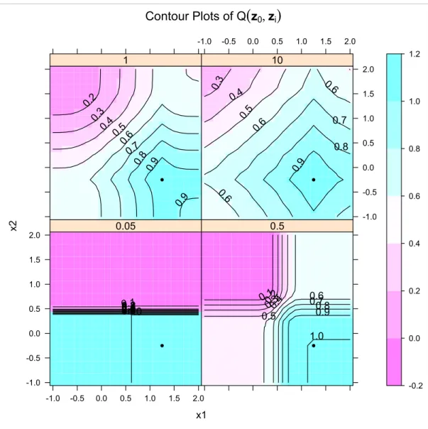
Figure 3.1 contains a training set (n= 500) from the XOR data in the mlbench package in R. We constructed four stump ensembles on these data using σ = 0.05,0.5,1,10. Next we

3.4. VARIABLE RANDOMNESS STUMP ENSEMBLES 38

generated a test set that consisted of a grid of points over the same domain as the XOR data.

We fixed one point in this grid to be z0 and calculatedQ(z0,zi) for each of the remainingzi

in the grid. We used these values to construct contour plots ofQ(z0,z) relative to the point

z0. These are shown in Figure 3.2.

-1.0 -0.5 0.0 0.5 1.0 -1.0 -0.5 0.0 0.5 1.0

XOR Training Data

x1

x2

Figure 3.1: Training set (n= 500) used to construct stump ensembles.

The contours in Figure 3.2 represent the proportion of times each point lies in the same half

of a stump in each ensemble as the pointz0. Hence, the 0.9 contour represents points that are

3.4. VARIABLE RANDOMNESS STUMP ENSEMBLES 39 Contour Plots of Q

(

Figure 3.2: Contour plots of Q(z0,z). Each panel is labeled according to the value of σ used

3.5. CONCLUSION 40

points that are close toz0 and the 0.1 contour represents points that are far from z0.

Note that forσ = 10 in Figure 3.2 the contours indeed resemble those we would obtain from the L1 metric, as they are roughly diamond shaped and even spaced away from the point

z0. When σ = 0.05, the stump ensemble consists almost entirely of stumps that split the

data onx2 near 0.5. In this sense the ensemble is essentially acting as a single stump. With

intermediate amounts of randomness (σ = 0.5,1) the ensemble is more adaptive to the local structure of the two classes by identifying only the points in the lower right as being close to

z0.

3.5

Conclusion

In this chapter we have investigated the effect of varying amounts of randomness in tree

en-sembles. Since full tree ensembles pose significant obstacles to direct analytical treatment,

we examined the simpler method of stump ensembles. We argued that extreme randomness

is not necessarily beneficial, as in the case of stump ensembles complete randomness simply

recreates a kernel method using theL1metric. Subsequently, we argued empirically that

mod-erate amounts of randomness aids performance by allowing the distance metric 1−Q(zi,zj)

to adapt itself to the local structure of the conditional density of the response y.

An important question is whether these metrics must be estimated via a randomized tree

ensemble, or whether they can be calculated directly. We have considered this question in some

depth but could not achieve any meaningful results. In general, the precise metric one obtains

will be different depending on the particular randomization strategy used. Additionally, the

extreme non-linearity inherent in decision trees makes a theoretical analysis challenging. Thus,

it remains an open question whether there is a deterministic route to calculating the values

Chapter 4

Local Models Using Tree Ensemble

Weights

4.1

Introduction

The previous chapters developed the idea that tree ensembles are fitting weighted averages of

the training points, where the weights are determined by a particular locally adaptive distance

metric. This means that the predicted value of a tree ensemble atx0(for a continuous response

variabley) is ˆ y0 = n X i=1 Q(x0,xi)yi.

The form of this model is simply that of a locally constant model. But this naturally leads us

to ask if we might use these weights in some other fashion. Given the weights (or distances,

if you prefer)Q(x0,xi), we might apply them to any model that accepts weights.

4.2. FITTING LOCAL MODELS 42

In this chapter we briefly explore the possible benefits to using the distance metricQ(x0,xi)

as weights in locally linear models. By this we simply mean fitting weighted linear regression

models using the values Q(x0,xi) as weights.

4.2

Fitting Local Models

Consider training data that conform to a traditional regression setting, (y,X) and a corre-sponding test point (y0,x0). A standard linear model using these data has the formy=Xβ+

where the errors are typically assumed to be independent and normally distributed. The

co-efficients are found using least squares with the familiar formula βˆ = (X0X)−1X0y. This model can be altered to become a local mode by adding weights to each of the training

points. In particular, given a diagonal weight matrix W, the coefficient vector is now found

via βˆ= (X0W X)−1X0W y.

We propose using the tree ensemble distancesQ(x0,xi) as the diagonal elements of the matrix W. To accomplish this we use the R implementation of Leo Breiman’s RandomForest software.

The R functionrandomForest1 allows us to estimate the valuesQ(x0,xi) using only the

out-of-bag samples. This means that the function returns a matrix of values that represent the

proportion of times that the two observations land in the same terminal node, and that these

proportions are estimated using only those trees for which this pair of observations are both

“out-of-bag”, that is not included in the bootstrap sample for that tree. Once we have the

values Q(x0,xi) to be used in the matrixW we estimate the coefficientsβˆ and use them to

predict the value y0 at x0. This process is repeated for each test point, so a distinct set of

coefficients βˆ is estimated for each test point.

One issue that arises in implementing this procedure is that tree ensembles are often used

in situations where the number of covariates is very large. While the tree ensemble easily

1

4.2. FITTING LOCAL MODELS 43

handles large numbers of covariates, traditional linear models can have difficulties, specifically

in inverting the matrixX0X. Generally, the solution to this problem is some form of

regular-ization. Instead, we will utilize another feature of the randomForestthat measures the local

variable importance for each training point. What this means is that for each training point

we examine the trees in the ensemble for which that observation is out-of-bag. Next we pick

a variable, say the mth, and permute its values (i.e. permute that column in the matrix X). Then we run our training observation down each of the trees and record the number of votes

for the correct class (classification) or the mean squared error (regression). This is repeated

over several permutations of the mth variable and the results averaged. The difference be-tween this and the corresponding value for the un-permuted version of X is the importance

of variablem on this training observation.

We can estimate the local variable importance for our independent test pointx0by combining

the local variable importance values of the training points with their proximities to the test

point x0. Let p be the vector of proximities of the test point to each of the training points

as estimated by the tree ensemble and letL be the matrix of local variable importance scores

for the training observations. The columns of L correspond to the training observations and

the rows to variables. Take the point-wise product of each row of L with the vector p and

sum along the rows of the resulting matrix. This vector is the local variable importance for

the independent test point. The rationale here is that the local variable importance at our

test point is estimated by the (weighted) average of the local variable importance at training

pointsclose to our test point. We can now use this vector to select only them most relevant covariates to use when we fit our local linear model. Specifically, we would only use the m

columns of X corresponding to the m highest local variable importance values for the test point.

This procedure actually allows us to significantly enlarge the number of covariates we can

consider. Since the tree ensemble method does not suffer from over-fitting problems when

4.3. NUMERICAL