The University of Sydney Business School The University of Sydney
BUSINESS ANALYTICS WORKING PAPER SERIES
Random Effects Models with Deep Neural Network Basis
Functions: Methodology and Computation
Minh-Ngoc Tran, Nghia Nguyen, David J. Nott and Robert Kohn
Abstract
Deep neural networks (DNNs) are a powerful tool for functional approximation. We describe flexible versions of generalized linear and generalized linear mixed models incorporating basis functions formed by a deep neural network. The consideration of neural networks with random effects seems little used in the literature, perhaps because of the computational challenges of incorporating subject specific parameters into already complex models. Efficient computational methods for Bayesian inference are developed based on Gaussian variational approximation methods. A
parsimonious but flexible factor parametrization of the covariance matrix is used in the Gaussian variational approximation. We implement natural gradient methods for the optimization, exploiting the factor structure of the variational covariance matrix to perform fast matrix vector multiplications in iterative conjugate gradient linear solvers in natural gradient computations. The method can be implemented in high
dimensions, and the use of the natural gradient allows faster and more stable convergence of the variational algorithm. In the case of random effects, we compute unbiased estimates of the gradient of the lower bound in the model with the random effects integrated out by making use of Fisher's identity. The proposed methods are illustrated in several examples for DNN random effects models and high-dimensional logistic regression with sparse signal shrinkage priors.
Keywords. Factor models; Reparametrization gradient; Stochastic optimization; Variational approximation.
February 2018
BA Working Paper No: BAWP-2018-01
Random effects models with deep neural network
basis functions: methodology and computation
Minh-Ngoc Tran
∗, Nghia Nguyen, David J. Nott and Robert Kohn
Abstract
Deep neural networks (DNNs) are a powerful tool for functional approx-imation. We describe flexible versions of generalized linear and generalized linear mixed models incorporating basis functions formed by a deep neural net-work. The consideration of neural networks with random effects seems little used in the literature, perhaps because of the computational challenges of in-corporating subject specific parameters into already complex models. Efficient computational methods for Bayesian inference are developed based on Gaus-sian variational approximation methods. A parsimonious but flexible factor parametrization of the covariance matirx is used in the Gaussian variational approximation. We implement natural gradient methods for the optimization, exploiting the factor structure of the variational covariance matrix to perform fast matrix vector multiplications in iterative conjugate gradient linear solvers in natural gradient computations. The method can be implemented in high dimensions, and the use of the natural gradient allows faster and more stable convergence of the variational algorithm. In the case of random effects, we compute unbiased estimates of the gradient of the lower bound in the model with the random effects integrated out by making use of Fisher’s identity. The proposed methods are illustrated in several examples for DNN random effects models and high-dimensional logistic regression with sparse signal shrinkage priors.
Keywords. Factor models; Reparametrization gradient; Stochastic optimiza-tion; Variational approximation.
1
Introduction
Deep neural network modeling provides a powerful technique for approximating mul-tivariate functions, and has become increasingly popular recently. DNNs have been applied successfully in fields such as image processing, computer vision and language
recognition. See Schmidhuber (2015) for a historical survey of DNNs and Goodfel-low et al. (2016) for a more comprehensive recent discussion. Polson and Sokolov (2017) provide a Bayesian perspective on DNN methodology and explain its connec-tion to statistical techniques such as principal component analysis and reduced rank regression.
This paper considers generalized linear models (GLMs) and generalized linear mixed model (GLMMs) using DNNs as a way to efficiently transform a vector of p
raw covariates X = (X1, ..., Xp)> into a new vector of m predictors Z in the model.
We refer to these DNN-based versions of GLM and GLMM as flexible GLM (fGLM) and flexible GLMM (fGLMM), respectively. A conventional GLM uses a link function that links the conditional mean of the response variable Y to a linear combination of the predictors Z = φ(X) = (φ1(X), ..., φm(X))>, with each φj(X) a function of X.
We refer to the original raw input variables Xj as covariates, and refer to the
trans-formationsφj(X) as predictors. Usually in conventional GLMs the φj(X) are chosen
a prioriin some way, but here we are concerned with learning an appropriate Z from data, and in the machine learning literature the predictors Z are commonly referred to as learned features. If a deep multi-layer perceptron is used for transforming the covariates, then Z has the form
Z =fL
WL, fL−1 WL−1,· · ·f1(W1, X)· · ·
. (1)
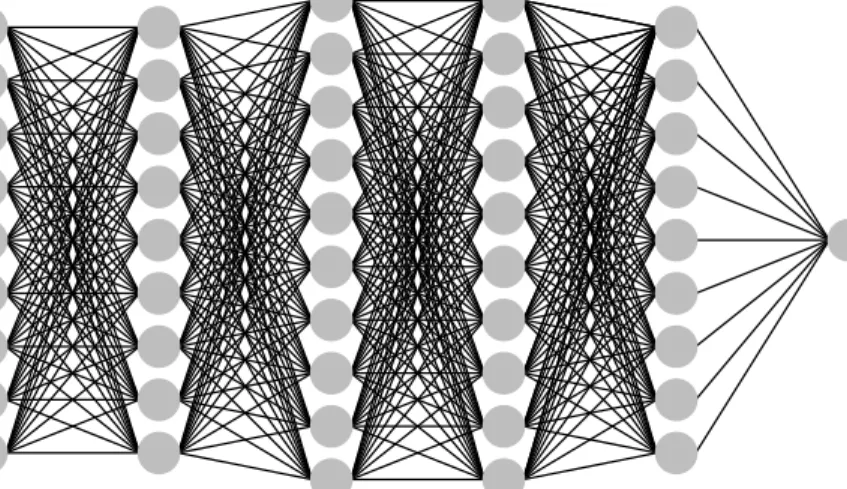
which is often graphically represented by a network as in Figure 1. Each vector-valued
●
●
●
●
●
●
●
●
●
x1 x2 x3 x4 x5 x6 x7 x8 x9●
●
●
●
●
●
●
●
●
●
●
●
●
●
●
●
●
●
●
●
●
●
●
●
●
●
●
●
●
●
●
●
●
●
●
●
●
●
●
OutputFigure 1: Graphical representation of a layered composition function with L= 4 hidden layers. The input layer represents 9 raw covariates X. The last hidden layer (hidden layer 4) represents the predictors Z.
layers in the network,w=(W1,...,WL) is the set of weights, and we defineZ0=X. The
function fj(Wj,Zj−1) is assumed to be of the formhj(WjZj−1) where Wj is a matrix
of weights for layer j and hj(·) is a scalar function, called the activation function.
Applying hj to a vector should be understood component-wise. For a discussion of
alternative kinds of architectures for deep neural networks see for example Goodfellow et al. (2016). The architecture (1) provides a powerful way to transform the raw covariate data X into summary statistics Z that have some desirable properties. In the fGLM, we link the conditional mean of the response ξ=E(Y|X) to a linear combination of Z
g(ξ) =β0+Z>β.e
and the model parameters consist of w,β and other possible parameters such as any dispersion parameters. Section 2.2 defines fGLMM models by adding random effects to fGLM models. Such models are designed to model within-subject dependence. The use of neural network basis functions in the context of mixed effects models seems not considered much in the literature. Lai et al. (2006) is the earliest work that we know of that deals with a neural network basis and random effects, in the context of modelling pharmacokinetic data. They consider neural networks with only one hidden layer, however.
Estimating complex and high-dimensional models like fGLM and fGLMM is chal-lenging. This article develops Bayesian inference based on variational approximation, which provides an approach to approximate Bayesian inference that is useful for many modern applications involving complex models and large datasets. When the approx-imation of the posterior distribution is Gaussian, parsimonious but flexible methods for parametrizing the covariance matrix are needed if the approach is to be useful for problems with a high-dimensional parameter. Here we consider factor parametriza-tions (Bartholomew et al., 2011) which are often effective for describing dependence in high dimensional settings. We discuss efficient methods for performing the variational optimization in this context using the natural gradient (Amari, 1998) by leveraging the factor structure and using iterative conjugate gradient methods for solving large linear systems. In the “isotropic” case with a one-factor decomposition and constant variance for the idiosyncratic noise components, we show that the natural gradi-ent can be computed analytically and efficigradi-ently without iterative conjugate gradigradi-ent methods which leads to a particularly simple Gaussian variational method for fitting high-dimensional models that can often be adequate for predictive inference.
Ong et al. (2017a) recently considered Gaussian variational approximation with a factor covariance structure using stochastic gradient approaches to the optimization. Their approach uses the so-called reparametrization trick (Kingma and Welling, 2013; Rezende et al., 2014) and its modification by Roeder et al. (2017) for estimating gra-dients of the variational objective. However, for certain models where the variational objective is very challenging to optimize, first-order optimization methods such as those considered in Ong et al. (2017a) may be very slow to converge. Ong et al. (2017b) earlier considered natural gradient methods for Gaussian variational
approx-imations using a factor covariance structure. However, their work was in the context of likelihood-free inference methods with a parameter of dimension at most a few hundreds, and the approach they develop does not scale to larger problems. The cur-rent work shows how the natural gradient Gaussian variational approximation with factor covariance can be implemented even in very high dimensions.
Much of the recent literature relevant to our training method occurs in the field of deep learning. Martens (2010) considers second-order optimization methods in deep learning and describes Hessian-free optimization methods, adapting a long history of related methods in the numerical analysis literature to that context. A detailed discussion of the connections between natural gradient methods and second order optimization methods is given in Martens (2014). Pascanu and Bengio (2014) con-siders the use of the natural gradient in deep learning problems and its connections with Hessian-free optimization, but like Martens (2010) their work is not specifically concerned with variational objectives. Fan et al. (2015) consider how to implement Hessian-free methods for the case of a variational objective function and Gaussian approximating family. Similarly to our development here, they consider using conju-gate gradient linear solvers as an efficient solution to the difficult matrix calculations that occur in a naive formulation of second-order methods. By a reparametrization approach they are able to obtain estimates of Hessian vector products. They do not consider factor parametrizations of the covariance structure, however. Here we leverage the factor covariance structure to calculate the matrix vector products we need directly, without the need to store large matrices. Recently Regier et al. (2017) consider a second order trust region method for black box variational inference. They show that while their approach may be more expensive per iteration than common first-order methods for variational Gaussian approximation such as those implemented in Titsias and L´azaro-Gredilla (2014) and Kucukelbir et al. (2017), it reduces total computation time and provably converges to a stationary point. It may be useful to consider how to exploit a factor parametrization of the covariance structure in the framework they develop, but this is not considered here.
We illustrate the DNN-based flexible models and the training method in a range of experimental studies and applications, with a focus on models involving complex hierarchically structured priors and datasets of only moderate size where quantifica-tion of uncertainty is important. Many successful applicaquantifica-tions of DNN are in image processing and speech recognition, where the datasets are large and have some spe-cial domain-application characteristics such as association between the local pixels in an image. Skepticism has sometimes been expressed about whether DNN methods are useful for applications involving limited data where uncertainty quantificaiton is the focus. The main conclusion in our examples is that the DNN-based regression models fGLM and fGLMM perform very well in terms of prediction accuracy, pro-vided appropriate attention is paid to regularization methods, prior distributions and computational algorithms.
and fGLMM. Section 3 describes the natural gradient Gaussian variational approxi-mation method, Section 4 highlights advantages of our Bayesian treatment. Section 5 presents experimental studies and applications. Section 6 concludes. The Appendix gives details of the VB natural gradient computation and more details of an example.
2
Flexible regression models with DNN
2.1
Flexible generalized linear models
Consider a dataset D={(yi,xi),i= 1,...,n} with yi the response and xi= (xi1,...,xip)>
the vector of p covariates. We also use y and x to denote a generic response and a covariate vector, respectively. Consider a neural net with the input vector x and a scalar output as represented in Figure 1. Denote by zj=φj(x,w), j= 1,...,m, the
units in the last hidden layer, wherew is the weights up to the last hidden layer, and
β= (β0,β1,...,βm)> are the weights that connect the zj to the output
N(x,w,β) =β0+β1z1+...+βmzm=β0+βe>z
with βe= (β1,...,βm)> and z= (z1,...,zm)>.
We assume that the conditional density p(y|x) has an exponential family form
p(y|x) = exp y$−b($) φ +c(φ, y) (2) with the canonical parameter $ and the dispersion parameter φ. Let g(·) be the link function that links the conditional mean ξ=ξ(x) =E(y|x) to a function of the covariates x. In the conventional GLM, g(ξ) is assumed to be a linear combination of x. In order to achieve flexibility and capture possible non-linear effects that x has onξ, we propose the more flexible model
g(ξ) = β0 +βe>z =N(x, w, β). (3)
In our later examples we use the canonical link function where $=g(ξ), which is the log link for Poisson responses and the logit link for binomial responses. The predictors (learned features)zj efficiently capture the important non-linear effects of the original
raw covariates x ong(ξ).
The model (3) is flexible, but can be hard to interpret. It may be useful in this respect to introduce additional structure. We might partition the covariates as
x= (x(1)T,x(2)T)T so that x(1) and x(2) have non-linear and linear effects respectively
ong(ξ), so that
whereβ(1)parametrizes a nonlinear effect w.r.t. the covariatesx(1)andβ(2)parametrizes
the linear effects w.r.t. the covariates x(2). Writeβ= (β(1),β(2)). We refer to the
gen-eral regression model with the exponential family form response distribution (2) and the mean model (3) or (4) as flexible GLM (fGLM).
The vector of model parameters θ consists of w, β and possibly dispersion pa-rameters φ if φ is unknown. The density p(y|x) in (2) is now a function of θ:
p(y|x) =p(y|x,θ). Given a datasetD, the likelihood function is
L(θ) =
n
Y
i=1
p(yi|xi, θ), (5)
and likelihood-based inference methods, including Bayesian methods, are easily ap-plied.
2.2
Flexible generalized linear mixed models
Consider a panel dataset D={(yit,xit),t= 1,...,Ti,i= 1,...,n} with yit the response
and xit the vector of covariates of subject i at time t. Generalized linear mixed
models (GLMM) use random effects to account for within-subject dependence. Let
zit,j=φj(xit,w), j = 1,...,m, be the units in the last hidden layer of a neural net,
zit= (zit,1,...,zit,m)>. Similarly to GLMM, to account for within-subject dependence,
we propose to link the conditional mean of yit, given xit, to the predictors zit,j as
follows
g(ξit) = β0 +αi0+ (β1+αi1)zit,1+...+ (βm+αim)zit,m
= N(xit, w, β+αi) (6)
where αi= (αi0,...,αim)> are random effects that reflect the characteristics of subject
i. The variation between the subjects is captured in the distribution ofαi. Our paper
assumes αi∼ N(0,Γ) but more flexible distributional specifications for the random
effects can also be considered.
Similarly to the previous section, a more interpretable model can be developed if some additional structure is assumed. Partition the covariates xit as (x
(1)
it T
,x(2)it T)T where x(1)it and x(2)it have non-linear and linear effects respectively on g(ξit):
g(ξit) = N(x (1) it , w, β (1)) + (α i+β(2))>x (2) it (7)
whereβ(1) parametrizes fixed non-linear effects for x(1)
it , andβ(2) andαi are fixed and
random linear effects w.r.t. the covariates x(2)it . Write β= (β(1),β(2)). The model
parameters θ include w, β, Γ and any dispersion parameters φ if unknown. We refer to the panel data model with the distribution (2) and the link (6) or (7) as flexible GLMM (fGLMM).
The likelihood for the fGLMM is L(θ) = n Y i=1 Li(θ) (8)
with the likelihood contribution
Li(θ) =p(yi|xi, θ) = Z p(yi|xi, w, β, φ, αi)p(αi|Γ)dαi = Z Ti Y t=1 p(yit|zit, β, φ, αi)p(αi|Γ)dαi. (9)
Section 3 describes a VB algorithm for fitting the fGLMM.
The likelihood for the fGLMM described in (8) and (9) is intractable, because the integral in (9) cannot be computed analytically, except for the case where the conditional distribution of yit given zit is normal. However, we can estimate each
likelihood contribution Li(θ) unbiasedly using importance sampling, and this allows
estimation methods for intractable likelihoods, such as the block pseudo-marginal MCMC of Tran et al. (2016) or the VB method of Tran et al. (2017), to be used. We consider here an alternative VB method based on the reparametrization trick in Section 3.1, which utilizes the information of the gradient of the log-likelihood computed by the back-propagation algorithm. By Fisher’s identity (Gunawan et al., 2017), the gradient of the log-likelihood contribution ∇θ`i(θ), `i(θ) = logLi(θ) with
Li(θ) in (9), is ∇θ`i(θ) = Z ∇θ log Ti Y t=i p(yit|zit, β, φ, αi)p(αi|Γ) ! p(αi|θ, yi, xi)dαi, (10)
where p(αi|θ,yi,xi) is the conditional distribution of the random effects αi given
data (yi,xi) and θ. The gradient inside the integral (10) can be computed by
back-propagation, and then the integral can be estimated easily by importance sampling.
3
Gaussian variational approximation with factor
covariance structure
This section describes the natural gradient Gaussian variational approximation method. Let D be the data and θ∈Θ the vector of unknown parameters. Bayesian inference about θ is based on the posterior distribution with density function
π(θ) =p(θ|D) =p(θ)L(θ)
with p(θ) the prior, L(θ) =p(D|θ) the likelihood function and p(D) =R
p(θ)L(θ)dθ
the marginal likelihood. In all but a few simple cases the posteriorπ(θ) is unknown, partly because p(D) is unknown, which makes it challenging to carry out Bayesian inference.
In this work, we are interested in variational approximation methods, which are widely used as a scalable and computationally effective method for Bayesian compu-tation (Bishop, 2006; Blei et al., 2017). We will approximate the posterior π(θ) by a distribution with density qλ(θ) within some family of standard distributions. For
example, if qλ(θ) =N(θ;µ,Σ), the density of a multivariate normal distribution with
mean vector µ and covariance matrix Σ, then λ= (µ,Σ). The best λ is chosen by minimizing the Kullback-Leibler divergence between qλ(θ) and π(θ)
KL(λ) = Z qλ(θ) log qλ(θ) π(θ)dθ = Z qλ(θ) log qλ(θ) p(θ)L(θ)dθ+ logp(D) = −LB(λ) + logp(D), (11) where LB(λ) = Z qλ(θ)log p(θ)L(θ) qλ(θ) dθ
is a lower bound on logp(D). Minimizing KL(λ) is therefore equivalent to maximizing the lower bound LB(λ). If we can obtain an unbiased estimator ∇\λLB(λ) of the
gradient of the lower bound, then we can use stochastic optimization to maximize LB(λ), as in Algorithm 1 below.
Algorithm 1. • Initialize λ(0) and stop the following iteration if the stopping
criterion is met.
• For t= 0,1,..., compute λ(t+1)=λ(t)+a
t∇\λLB(λ(t)).
The learning rate sequence {at}in Algorithm 1 should satisfy the Robbins-Monro
conditions,at>0,Ptat=∞ andPta2t<∞(Robbins and Monro, 1951). Choice ofat
is discussed later on in some detail.
3.1
Reparametrization trick
As is typical of stochastic optimization algorithms, the performance of Algorithm 1 depends greatly on the variance of the noisy gradient. Techniques for variance reduction are needed. We will use the so-called reparametrization trick (Kingma and Welling, 2013; Rezende et al., 2014) in this paper, and its modification by Roeder et al. (2017), who generalized ideas considered in Han et al. (2016) and Tan and Nott (2017).
Suppose that for θ∼qλ(·), there exists a deterministic function g(λ,) such that
N(θ;µ,Σ) thenθ=µ+Σ1/2with∼N(0,I) andI the identity matrix. Writing LB(λ)
as an expectation with respect to p() gives LB(λ) =E
h(g(,λ))−logqλ(g(,λ))
,
where E(·) denotes expectation with respect to p(), h(θ) := log(p(θ)L(θ)).
Differ-entiating under the integral sign and simplifying as in Roeder et al. (2017) gives
∇λLB(λ) =E
∇λg(λ,)∇θ{h(g(,λ))−logqλ(g(,λ))}
. (12)
The gradient (12) can be estimated unbiasedly using i.i.d sampless∼p(·),s=1,...,S,
as \ ∇λLB(λ) = 1 S S X s=1 ∇λg(λ,s)∇θ h(g(λ,s))−logqλ(g(λ,s)) . (13)
The gradient estimator (13) has the advantage that if the variational family is rich enough to contain the exact posterior, so that exp(h(θ))∝qλ(θ) at the optimal λ,
then the estimator (13) is exactly zero at this optimal value even for s= 1 where we use just a single Monte Carlo sample fromp(). Reparametrized gradient estimators
are much more efficient than alternative approaches to estimating the lower bound gradient, partly because they take into account information from∇θh(θ). For further
discussion we refer the reader to Roeder et al. (2017).
3.2
Natural gradient
It is well-known that the ordinary gradient ∇λLB(λ) does not adequately capture
the geometry of the approximating family qλ(θ) (Amari, 1998). A small Euclidean
distance between λ and λ0 does not necessarily mean a small Kullback-Leibler diver-gence between qλ(θ) and qλ0(θ). Rao (1945) was the first to point out the importance of using the geometrical information on the manifold of a statistical model, and in-troduced the Riemannian metric on this manifold induced by the Fisher information matrix. Amari (1998) shows that the steepest direction for optimizing the objective function LB(λ) on the manifold formed by the familyqλ(θ) is directed by the so-called
natural gradient which is defined by pre-multiplying the ordinary gradient with the inverse of the Fisher information matrix
∇λLB(λ)natural =IF−1(λ)∇λLB(λ), (14)
with IF(λ) = covqλ(∇λlogqλ(θ)).
The use of the natural gradient in VB algorithms is considered, among others, by Sato (2001), Honkela et al. (2010), Hoffman et al. (2013), Salimans and Knowles (2013) and Tran et al. (2017). A simple demonstration of the importance of the
natural gradient can be found in Tran et al. (2017). The use of the natural gradient in deep learning problems is considered in Pascanu and Bengio (2014), who show the connection between natural gradient descent and other second-order optimization methods such as Hessian-free optimization.
The main difficulty of using the natural gradient is the computation ofIF(λ), and
the solution of linear systems involving this matrix, which is required to compute (14). The problem is more severe in high dimensional models because this matrix often has a large size. Some approximation methods, such as the truncated Newton approach, may be needed (Pascanu and Bengio, 2014). We consider in the next section an efficient method for computing IF(λ)−1∇λLB(λ) based on the use of iterative
conju-gate gradient methods for solving linear systems when the covariance matrix of the Gaussian variational approximation is parametrized by a factor model. We compute (14) by solving the linear system IF(λ)x=∇λLB(λ) for x using only matrix-vector
products involving IF(λ) where the matrix vector products can be done efficiently
both in terms of computation time and memory requirements by using the factor structure of the variational covariance matrix. In the special case of one factor with isotropic idiosyncratic noise the natural gradient in (14) can be computed analytically and efficiently.
3.3
Gaussian variational approximation with factor
covari-ance
We now describe in detail the Gaussian variational approximation with factor co-variance (VAFC) method of Ong et al. (2017a). The VAFC method considers the multivariate normal variational family qλ(θ) =N(µ,Σ) where Σ is parametrized as
Σ =BB>+D2. (15)
Here B is a d×f matrix (the factor loadings matrix) with d the dimension of
θ and f the number of factors, f d, and D is diagonal with diagonal entries ∆ = (∆1,...,∆d)>. ∆ is a vector of idiosyncratic noise standard deviations. Factor
structures are well known to provide useful parsimonious representations of depen-dence in high-dimensional settings (Bartholomew et al., 2011). We assumeB is lower triangular, i.e., Bij= 0 forj > i. Although imposing the constraint Bii>0 makes the
factor representation identifiable (Geweke and Zhou, 1996), we do not impose this constraint to simplify the optimization. The variational optimization simply locks onto one of the equivalent modes. An intuitive generative representation of the fac-tor structure that is the basis of our application of the reparametrization trick is the following: if we consider θ∼qλ(θ) =N(µ,BB>+D2), then we can represent θ
as θ=µ+B1+∆◦2 where = (>1,>2)>∼N(0,I), 1 and 2 have dimensions f and
d respectively, and ◦ denotes the Hadamard (element by element) product for two matrices of the same size. We can see from this representation that the latent vari-ables1 (the “factors”, which are low-dimensional) explain all the correlation between
the components, whereas component-specific idiosyncratic variance is being captured through 2.
The variational parameters are λ= (µ>,vec(B)>,∆>)> where we have written vec(B) for the vectorization of B obtained by stacking its columns from left to right. Ong et al. (2017a) show that the gradient of the lower bound takes the form
∇µLB(λ) =E ∇θh(µ+B1+∆◦2)+(BB>+D2)−1(B1+∆◦2) , (16) ∇BLB(λ) =E ∇θh(µ+B1+∆◦2)>1+(BB > +D2)−1(B1+∆◦2)>1 , (17) and ∇∆LB(λ) =E diag ∇θh(µ+B1+∆◦2)>2 +(BB > +D2)−1(B1+∆◦2)>2 , (18) where we have written diag(A) for the diagonal elements of a square matrix A. Here, the inverse matrix (BB>+D2)−1 can be computed efficiently; see (19). We note that in the expression for the gradient of B above, we should set to zero the upper triangular components which correspond to elements of B which are fixed at zero. Unbiased estimation of gradients for stochastic gradient ascent can proceed based on these expressions by drawing one or more samples from p() to estimate the
expectations.
3.4
Efficient natural gradient VAFC method
We now describe how to efficiently implement natural gradient optimization for the VAFC method. Ong et al. (2017b) have also considered a natural gradient method for Gaussian variational approximation with factor covariance. However, this was in the context of likelihood-free inference methods where the dimension ofθis low compared to the models of interest here, and they simply used naive methods for solving the linear systems involving IF(λ) required to compute the natural gradient. This is
impractical in high-dimensional problems, and here we demonstrate how to implement natural gradient VAFC whenθ is high-dimensional using conjugate gradient methods (see, for example, Stoer (1983)).
Write IF(λ) in partitioned form as
IF(λ) = I11 I21> I31> I21 I22 I32> I31 I32 I33 ,
where the blocks in the partition follow the partition of λ as λ= (µ>,vec(B)>,∆>)>. Because the upper triangle of B is fixed at zero the corresponding rows and columns ofIF(λ) should be omitted. Ong et al. (2017b) show thatI11=Σ−1,I21=I31=0,I22=
2(B>Σ−1B⊗Σ−1) (where ⊗denotes the Kronecker product), I
33= 2(DΣ−1)◦(Σ−1D)
and I32= 2(B>Σ−1D⊗Σ−1)Ed> where Ed is the d×d2 matrix that picks out the
diagonal elements of the d×d matrix A from its vectorization, so that Edvec(A) =
diag(A). To use a conjugate gradient linear solver to compute IF(λ)−1∇λLB(λ) we
simply need to be able to compute matrix vector products of the formIF(λ)x for any
vector x quickly without requiring to store the elements ofIF(λ).
This can be done provided we can do matrix vector products for the matrices I11,
I22,I33andI32. This is still difficult so we further approximateIF(λ) by settingI32=0
and replacingI33with ˜I33= 2(DΣ˜−1)◦( ˜Σ−1D) where ˜Σ is the diagonal approximation
to Σ obtained by setting its off-diagonal elements to zero. Using this approximation and I32= 0 we obtain a positive definite approximation ˜IF(λ) to IF(λ) which we use
instead of IF(λ) in the natural gradient.
Multiplications involving ˜I33 are simple since this matrix is diagonal, but we still
need efficient methods to compute matrix vector products forI11andI22. Considering
I11 first, we note that by using the Woodbury formula
I11 = Σ−1 =D−2−D−2B(I+B>D−1B)−1B>D−2, (19)
and then noting thatDis diagonal, and (I+B>D−2B) isf×f,fd, we can calculate
I11x= Σ−1x without needing to store any d×d matrix or do any dense d×d matrix
multiplications. Next, consider I22x for some vectorx. We note that
I22= 2(B>Σ−1B⊗Σ−1)x= 2vec(Σ−1x∗B>Σ−1B)
where x∗ denotes thed×f matrix such that x= vec(x∗) and where we have used the identity that for conformable matrices X,Y,Z, vec(XY Z) = (Z>⊗X)vec(Y). Then Σ−1x∗ is easily computed efficiently by the Woodbury formula, and similarly for
B>Σ−1B.
3.4.1 Special case of isotropy factor decomposition
We now consider the special case where the covariance matrix Σ is parameterized as Σ =BB>+c2I
d with B a vector and c a constant. In this case, the natural
gradi-ent (14) can be computed in closed form and the computational complexity is O(d). The detailed derivation can be found in the Appendix. This estimation method is computationally attractive, especially for cases where the dimension d is extremely large. Our experimental studies in Section 5 suggest that in some applications this method is able to produce a prediction accuracy comparable to the accuracy ob-tained by methods that use more flexible factor decomposition structures of Σ. A recent discussion of the phenomenon of richer variational families producing inferior performance in terms of predictive loss for neural networks models is given in Trippe and Turner (2018), with some theoretical insights into this phenomenon.
4
Practical recommendations in training DNN
mod-els
Our natural gradient Gaussian variational approximation method can be used as a general estimation method for any model. However, this section focuses on estimat-ing DL-based models, and discusses some implementation recommendations that we found useful in practice.
4.1
Bayesian treatment
Selecting the tuning parameters in DNN models can be challenging and we now develop some Bayes and empirical Bayes methods for this task for the models we consider. In fGLM and fGLMM we use ridge-type regularization priors, one for the inner weights w with shrinkage hyperparameter γw, and one for the output weights
β with shrinkage hyperparameter γβ. Adaptive regularizations that use different
shrinkage for different weights can also be used but we do not consider them here. Letβebeβ without the bias (also called intercept)β0, and
e
wbewwithout the biases. Let vec(we) be the vectorized version of we. We use the following priors
p(w)∝exp−γw 2 vec(we) > vec(we), p(β)∝exp−γβ 2 βe > e β.
To select the hyperparameters γw and γβ we use an empirical Bayes approach within
the iterative VB estimation method. Writing the Bayesian hierarchical model in the generic form
y|ψ, θ ∼ p(y|θ, ψ)
θ|ψ ∼ p(θ|ψ),
with y the data,θ the model parameters and ψ the hyperparameters to be selected. The marginal likelihood forψ isp(y|ψ)=Rp(θ|ψ)p(y|θ,ψ)dθ, which can be maximized using an EM-type algorithm (Casella, 2001). Given an initial value ψ(0),
ψ(k+1)= argmaxψEθ|y,ψ(k)logp(y,θ|ψ) .
HereEθ|y,ψ(k)(·) is the expectation with respect to the posterior distributionp(θ|y,ψ(k)).
It can be shown that the updating rule for γw and γβ is
γw(k+1) = dwe Eθ|y,ψ(k)(vec( e w)>vec( e w)), γ (k+1) β = dβe Eθ|y,ψ(k)(βe>βe) , (20)
where dwe and dβe denote the dimension of vec(we) and βe, respectively. In our VB framework, the expectation Eθ|y,ψ(k)(·) can be naturally approximated by the
expec-tation w.r.t. the current VB approximation qλ(k)(θ), then the updates in (20) can be
4.2
Other practical recommendations
We often use a fixed learning rate
at =0
τ
t (21)
where 0 is a small value, e.g. 0.01 and τ is some threshold from which the learning
rate is reduced, e.g. τ=200. It might also be useful to use some adaptive learning rate methods, and later we consider one method adapted from Ranganath et al. (2013) which is described in Ong et al. (2018). This learning rate is suitable for use with the natural gradient.
As a method of accelerating the stochastic gradient optimization we also consider use of the momentum method (Polyak, 1964). The update rule is
∇λLB = α∇λLB + (1−α)∇\λKL(λ(t))natural,
λ(t+1) = λ(t)+at∇λLB,
where α∈[0,1] is the momentum weight. The use of the moving average gradient
∇λLB helps remove some of the noise inherent in the estimated gradients of the lower
bound. See Goodfellow et al. (2016), Chapter 8, for a detailed discussion on the usefulness of the momentum method.
It is common in modern deep learning applications of neural network methods to implement early stopping in the optimization to avoid overfitting, even if regulariza-tion priors are used. We often observe that the training loss decreases steadily over the VB updates, while the validation loss starts increasing at some point. Therefore we also implement early stopping of the variational inference algorithm if the valida-tion loss on a test set has not decreased after a certain number of iteravalida-tions, and the set of model parameters with respect to the lowest validation loss is stored.
For initialization of variational parameters λ(0)= (µ(0),B(0),∆(0)), we follow Glorot and Bengio (2010) and initialize each weight in µ(0) byU(−q 6
m+n,
q
6
m+n) where the
weight connects a layer with m units to a layer with n units. The elements in B(0)
are initialized by N(0,0.0012) and the elements in ∆(0) are initialized by 0.001. It is
advisable to first standardize the input data so that each column has a zero sample mean and a standard deviation of one. Finally, we use the rectified activation function
h(x) =
(
x, if x >0,
0, else in all examples, if not otherwise stated.
5
Experimental studies and applications
To illustrate the prediction accuracy of fGLM and fGLMM, and the efficiency of our natural gradient training algorithms we consider a range of experimental studies and
applications. All the examples are implemented in Matlab and run on a desktop computer with i5 3.3 Ghz Intel Quad Core.
5.1
Experimental studies
5.1.1 Efficiency of the natural gradient
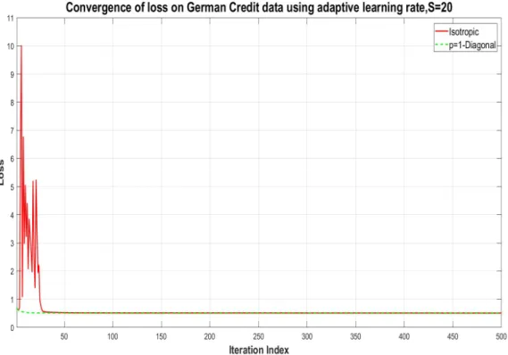
We use a German credit dataset with 1000 observations, of which 750 are used as the training data and the rest as the test data. This dataset is obtained from the UCI Machine Learning Repository, http://archive.ics.uci.edu/ml. The data consist of a binary response variable, credit status, which is good credit (1) or bad credit (0), together with 30 covariate variables such as education, credit amount, employment status, etc. We consider a simple logistic regression model for predicting the credit status, based on the covariates. We use an improper flat prior for the coefficients θ, i.e. p(θ)∝1.
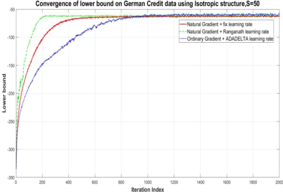
We first study the performance of the natural gradient method compared to the ordinary gradient method. Figure 2 shows the convergence of the lower bound of the ordinary gradient method and the natural gradient method using a single factor and isotropic idiosyncratic noise, i.e. Σ =BB>+c2I where B is a column vector as
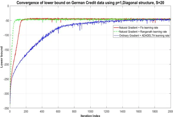
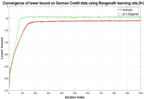
described in Section 3.4.1. For the ordinary gradient, we use the adaptive learning rate method ADADELTA of Zeiler (2012). For the natural gradient, we use both the fixed learning rate in (21) and the adaptive learning rate of Ong et al. (2018) (which is based on a similar method in Ranganath et al. (2013)). The figure shows that using both the natural gradient and adaptive learning rate speeds convergence. Figure 3 shows similar results for a one factor model with non-isotropic idiosyncratic noise, i.e. Σ =BB>+D2 for D diagonal. The results have a similar interpretation to before -the natural gradient speeds up convergence and -the adaptive learning rate is helpful. Figure 4 compares lower bounds for the one-factor parameterization with and without isotropic noise - the difference in the lower bounds evident in the figure shows the improvement in the posterior approximation brought by the more general variational family but Figure 5 shows that the predictive loss is similar.
5.1.2 Prediction accuracy of DL models
We generate data from two models
(M1) y = 5 + 3(X1+ 2X2)2+ 5X3X4+ 2X5+
(M2) y= 5 + 10X1 +X102
2+1 + 5X3X4+ 2X4+ 5X
2
4 + 5X5+
where ∼ N(0,1). For each model, we generate a training dataset of ntrain= 100,000
observations and a test dataset of ntest= 100,000 observations. For the first model
the Xi are generated from the uniform distribution U(−1,1), for the second model
Figure 2: Lower bound versus iteration number for the ordinary gradient and natural gradient methods: the variational family uses a covariance matrix with one factor and isotropic idiosyncratic noise.
zero and covariance matrix (0.5|i−j|)
i,j. In both models the relationship between y
and theXi is non-linear, and it is more difficult to predict the response in the second
model.
To measure the prediction accuracy, we use partial predictive score (PPS)
P P S=− 1
ntest
X
(xi,yi)∈test data
logp(yi|xi,bθ),
with θba point estimate of the model parameters, and mean squared error (MSE)
M SE= 1 ntest X (xi,yi)∈test data (yi−ybi) 2 ,
with byi a prediction of yi. In our fGLM, for the dataset generated from M1, we use
a neural net with the structure (5,10,10,1), i.e. the input layer has 5 variables, two hidden layers each has 10 units and one scalar output. For the dataset generated fromM2, we use a neural net with the structure (5,10,10,10,10,1), i.e. there are four
Figure 3: Lower bound versus iteration number for the ordinary gradient and natural gradient methods: the variational family uses a covariance matrix with one factor and non-isotropic idiosyncratic noise.
exploration. We use the one factor variational family with isotropic idiosyncratic noise and the natural gradient training method with fixed learning rate in (21). We compare the performance of fGLM to that of a linear model. Table 1 summarizes the results, which shows that fGLM outperforms the linear model in term of prediction accuracy. The RMSE of fGLM is close to 1, which is the best RMSE under the true model.
M1 M2
Method PPS MSE PPS MSE GLM 2.26 5.84 2.98 11.62 fGLM 0.83 1.34 0.86 1.39
Table 1: Performance of fGLM v.s. GLM in term of the partial predictive score (PPS) and the mean squared error (MSE). Both are evaluated on the test dataset.
Figure 4: Lower bound versus iteration number for the natural gradient method: comparison of variational families using covariance matrices with one factor and with and without isotropic diosyncratic noise.
5.1.3 Binary panel data simulation
We study the fGLMM on a simulation binary panel datasetD={(xit,yit);t=1,...,20;i=
1,...,1000} with xit the vector of covariates and yit the response of subject i at time
t. The response yit is generated from the following model:
ait = 2 + 3(xit,1−2xit,2)2−5 xit,3 (1 +xit,4)2 −5xit,5+bi+it, yit = ( 1, if ait>0, 0, otherwise,
wherebi∼N(0,0.1) is a random effect intercept representing charactersistics of subject
i and it∼ N(0,1) is random noise associated with reponses yit. The xit,j,j= 1,...,5,
are generated from a uniform distribution U(−1,1).
Figure 5: Prediction loss versus iteration number for the natural gradient method: comparison of variational families using covariance matrices with one factor and with and without isotropic diosyncratic noise.
this dataset yit|xit ∼ Binomial(1, µit) log µit 1−µit = N(xit, w, β+αi),
whereN(xit,w,β+αi) is the scalar output of a neural net with inputxit, inner weights
w and output weights β+αi. We assume that the random effects αi∼ N(0,Γ) with
Γ = diag(γ0,...,γm). The model parameters are θ= (w,β,γ0,...,γm). We use Gamma
priors on theγj, γj∼Gamma(a0,b0), and set the hyperparameters a0= 1 and b0= 0.1
in this example. The Appendix gives further details on training this model.
For each subject, we use the first 14 observations for training, next 3 observations for validation and the last 3 observations for testing. That is, we are interested in the within-subject prediction. The neural network has one hidden layer with 10 nodes, and we compare the fGLMM model with the logistic regression model with a random intercept.
We use two measures of predictive performance. The first is the partial predictive score (PPS), which is the average of the negative log-likelihood values. The second
is the misclassification rate. Let ¯θ be the mean of the VB approximation qλ(θ) after
convergence. Let bµαi in (31) be the mode of p(αi|yi,xi,θ¯), which can be used as the
prediction of the random effectsαi of individuali. Let (yit0,xit0) be a future data pair
and b µit0= 1 1+exp(−N(xit0,w,β+µbαi)) .
We set the prediction of yit0 as
b
yit0= 1 if and only if N(xit0,w,β+µbαi)≥0.
The classification error is MCR =XI
b
yit06=yit0/total number of future observations
with the sum over the test data points (yit0,xit0).
Table 2 summarizes the comparison of fGLMM and GLMM performance. The results clearly show that modelling covariate effects in a flexible way using the neural network basis functions is helpful here in terms of improving both PPS and MCR.
Model PPS MCR GLMM 1.24 17.57% fGLMM 0.13 5.27%
Table 2: Simulation binary panel dataset: Performance of fGLMM v.s. GLMM in term of the partial predictive score (PPS) and the misclassification rate (MCR). Both are evaluated on the test dataset.
5.2
Applications
5.2.1 High-dimensional logistic regression using the horseshoe prior
This application is concerned with high-dimensional logistic regression using a sparse signal shrinkage prior, the horseshoe prior (Carvalho et al., 2010). Here the variational optimization is challenging because of the strong dependence between local variance parameters and the corresponding coefficients. Using three real datasets we show that the natural gradient estimation method improves the performance of the approach described in Ong et al. (2017a).
Let yi∈ {0,1} be a set of binary responses with corresponding covariates xi=
(xi1,...,xip)>,i= 1,...,n. We consider a logistic regression model
log µi 1−µi
where µi= P(yi= 1|xi), β0 is an intercept and β= (β1,...,βp)> are coefficients. We
consider the setting where pis large, possibly pn, and use a shrinkage prior for β, the horseshoe prior (Carvalho et al., 2010). Specifically we assume β0∼N(0,10) and
βj|λj∼N(0,λ2jg
2) λ
j∼C+(0,1),
j= 1,...,p, where C+(0,1) denotes the half-Cauchy distribution. The parameters λ
j,
j=1,...,pare local variance parameters providing shrinkage for individual coefficients, and the parameter g is a global shrinkage parameter which can adapt to the overall level of sparsity. For g a half-Cauchy prior is assumed, g∼C+(0,1). The above prior
settings are the same as those considered in Ong et al. (2017a).
The parameterθconsists ofθ=(β0,β>,δ>,γ)>, whereδ=(δ1,...,δp)>=(logλ1,...,logλp)>,
and γ= logg. We consider Gaussian variational approximation for the posterior of
θ, using a factor covariance structure, for 3 gene expression datasets, the Colon,
Leukaemia and Breast cancer datasets found at http://www.csie.ntu.edu.tw/ ~cjlin/libsvmtools/datasets/binary.html. These three datasetsColon,Leukaemia
andBreasthave training sample sizes of 42, 38 and 38 and test set sizes of 20, 34 and 4 respectively. The number of covariates is p= 2000 for theColon data, and p= 7120 for the Leukaemia and Breast datasets. This means that for the Leukaemia and
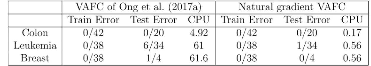
Breast datasets the dimension of θ is 14,242 so these are very high-dimensional ex-amples in terms of the parameter. These data were also considered in Ong et al. (2017a) where slow convergence in the variational optimization was observed using their method; we show here that a natural gradient approach offers a significant improvement.
VAFC of Ong et al. (2017a) Natural gradient VAFC Train Error Test Error CPU Train Error Test Error CPU
Colon 0/42 0/20 4.92 0/42 0/20 0.17
Leukemia 0/38 6/34 61 0/38 1/34 0.56
Breast 0/38 1/4 61.6 0/38 0/4 0.56
Table 3: Performance of the ordinary gradient VAFC and natural gradient VAFC methods on three cancer datasets. Training and test errors rates are reported as the ratio of misclassified data points over the number of data points. Computational time CPU (per 100 iterations) is measured in second.
Table 3 compares the performance of VAFC of Ong et al. (2017a) and our natural gradient VAFC training methods. The table shows the predictive performance and computational time on three cancer datasets. We ran VAFC withf=4 factors and use only a single sample to estimate the gradient of lower bound (S= 1) in two methods.
5.2.2 Flexible Poisson regression: bike sharing data
Bike-rental behavior is highly correlated to environmental and seasonal settings. Fanaee-T and Gama (2013) collected a dataset where the response data are hourly counts of rental bikes and the seven covariates are season (1: spring, 2: summer, 3: fall, 4: winter), holiday (1: if the day is holiday, 0: not), weekly day (1 if weekly day, 0 if weekend), weather, temperature, humidity and wind speed. The dataset is availalbe at the UCI Machine Learning Repository http://archive.ics.uci.edu/ml. To analyse this dataset, we use the following flexible Poisson regression model
yi|xi ∼ Poisson(µi)
log(µi) = N(xi, w, β).
The total 17379 observations are divided into a training dataset with 15000 observa-tions, and a test dataset with 2379 observations.
We consider a neural network with 8 layers, each with 7 units. The model is fitted using the isotropy natural gradient variational inference approach. The fitted model provides a PPS on the test set of−1005.2. Compared to a conventional Poisson linear generalized model whose PPS is -820.4, which suggests that the more flexible model is warranted.
5.2.3 A continuous panel data set: Cornwell and Rupert data
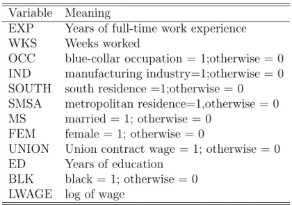
This section analyzes a continuous panel data set originally analyzed in Cornwell and Rupert (1988). This is a balanced panel dataset with 595 individuals and 4165 observations, in which each individual was observed for 7 years. The dataset is available from the website of the textbook Baltagi (2013). The variables are listed in Table 4.
We are interested in predicting the wage (on the log scale) of each individual, given the covariates. Let yit be a continuous variable indicating the log of wage of
person i with the vector of covariates xit in year t, t= 1,...,7. We use the following
flexible linear regression model with random effects
yit|xit ∼ N(µit, σ2)
µit = N(xit, w, β+αi),
whereN(xit,w,β+αi), β and αi have the same interpretation as in Section 5.1.3, and
σ2 is the variance of noise.
Since we are interested in within-subject prediction, for each individual, we use the first 4 observations as training data, the next 1 observation for validation data and the last 2 observations for test data. We use a neural network with 2 hidden layers 5 nodes each; this structure was selected after some experiments. We compare the performance of fGLMM to the linear regression model with a random effect, using PPS and MSE as evaluation metrics.
Variable Meaning
EXP Years of full-time work experience WKS Weeks worked
OCC blue-collar occupation = 1;otherwise = 0 IND manufacturing industry=1;otherwise = 0 SOUTH south residence =1;otherwise = 0
SMSA metropolitan residence=1,otherwise = 0 MS married = 1; otherwise = 0
FEM female = 1; otherwise = 0
UNION Union contract wage = 1; otherwise = 0 ED Years of education
BLK black = 1; otherwise = 0 LWAGE log of wage
Table 4: Cornwell and Rupert data: variables and their meaning
Table 5 summarizes the results, which again show that using the neural network as the basis functions to model covariate effects in a flexible way can significantly improve both PPS and MSE.
Model PPS MSE GLMM 0.05 0.18 fGLMM -0.87 0.05
Table 5: Cornwell and Rupert data: Performance of fGLMM v.s. GLMM in term of the partial predictive score (PPS) and the mean square error (MSE). Both are evaluated on the test dataset.
6
Discussions and conclusions
This paper is concerned with flexible versions of generalized linear and generalized linear mixed models where DNN methodology is used to automatically choose trans-formations of the raw covariates. The challenges of Bayesian computation have been addressed using variational approximation methods with a parsimonious factor co-variance structure. In the case of random effects models we are able to estimate the gradient of the log likelihood unbiasedly with the random effects integrated out efficiently using Fisher’s identity. We have demonstrated that a natural gradient ap-proach to the variational optimization with this family of approximations is feasible even in high dimensions using iterative conjugate gradient methods for solving large
positive definite linear systems in computation of the natural gradients. Using simu-lation and real datasets and several different models we show that the improvement that these methods can bring in terms of speed of convergence and computation time are substantial, and that the use of neural network basis functions with random effects is a class of models that deserve more consideration in the literature.
Appendix
Isotropic natural gradient VB estimation method
This section presents in detail the isotropic natural gradient VB estimation method for estimating a posterior distribution π(θ)∝exp(h(θ)), h(θ) = log(p(θ)L(θ)). With the VB approximationqλ(θ) =N(θ;µ,Σ), Σ =bb>+c2Id, the vector of the VB parameters
is λ= (µ>,b>,c)>. The lower bound LB(λ) =Eθ∼qλ h(θ)−logqλ(θ) =E h(g(,λ))−logqλ(g(,λ)) ,
whereθ=g(λ,)=µ+b1+c2 with a scalar1 andd-vector2,=(1,>2)
>∼N(0,I
d+1).
The ordinary gradient of the lower bound
∇λLB(λ) =E
∇λg(λ, )∇θ{h(θ)−logqλ(θ)} |θ=g(,λ)
,
which is estimated unbiasedly using i.i.d samples s∼ N(0,Id+1), s= 1,...,S as
\ ∇λLB(λ) = 1 S S X s=1 ∇λg(λ, s)∇θ h(θ)−logqλ(θ) |θ=g(s,λ). (22)
It’s easy to see that
∇λg(λ,) = Id 1Id >2 ,
while the gradient∇θh(θ) depends on the model being estimated, and finally by (29)
∇θlogqλ(θ) =−Σ−1(θ−µ) =−
1
c2(θ−µ)+
b>(θ−µ)
c2+b>b b.
In order to implement the natural gradient VB algorithm we need the information matrix IF(λ) = covqλ(∇λlogqλ(θ)), where
logqλ(θ)∝ − 1 2log|Σ|− 1 2(θ−µ) > Σ−1(θ−µ).
Let U=U(x) be a matrix-valued function of a scalar x, and g(U) be a real-valued function of U. By the chain rule (Petersen and Pedersen, 2012)
∇x g(U(x)) = trh∇U g(U) > ∇x U(x) i .
Note that∇U(a>U−1b) =−U−1ab>U−1 (Petersen and Pedersen, 2012), we have
∇b
(θ−µ)>Σ−1(θ−µ)=−2Σ−1(θ−µ)(θ−µ)>Σ−1b. (23) Because ∇U(log|U|) =U−1, we have ∇x(log|U|) = tr(U−1∇xU). Then
∇b log|Σ|= 2Σ−1b. (24) Similarly, ∇c log|Σ|= 2c×tr(Σ−1) (25) and ∇c (θ−µ)>Σ−1(θ−µ)=−2c(θ−µ)>Σ−2(θ−µ). (26) So ∇λlogqλ(θ) = ∇µlogqλ(θ) ∇blogqλ(θ) ∇clogqλ(θ) = Σ−1(θ−µ) −Σ−1b+ Σ−1(θ−µ)(θ−µ)>Σ−1b −c×tr(Σ−1) +c(θ−µ)>Σ−2(θ−µ) . (27)
Let X= Σ−1(θ−µ)∼ N(0,Σ−1), and using the results on cubic and quadratic forms
of a Gaussian random vector (Petersen and Pedersen, 2012), it can be shown that
IF(λ) = Σ−1 O d×d Od×1 Od×d Σ−1bb>Σ−1+ (b>Σ−1b)Σ−1 2cΣ−2b O1×d 2cb>Σ−2 2c2tr(Σ−2) . (28)
Now note that
Σ−1 = (bb>+c2I)−1 = 1 c2 I− 1 c2+b>bbb > = 1 c2 I−αbb > (29) and Σ−1b=αb,
with α= 1/(c2+b>b). The Fisher information matrix in (28) can be written as
IF(λ) = Σ−1 O d×d Od×1 Od×d A u O1×d u> ω
with A = Σ−1bbTΣ−1+ (bTΣ−1b)Σ−1 = α(b >b) c2 Id+α 2 1− b >b c2 bb> u = 2cΣ−2b= 2cα2b ω = 2c2tr(Σ−2) = 2 c2 d−1 + ( c 2 c2+b>b) 2 = 2 c2 d−1 + (c2α)2. Hence, IF−1(λ) = Σ−1 Od×(d+1) O(d+1)×d A u u> ω −1 with A u u> ω −1 = A−1+ω−u>1A−1uA −1uu>A−1 − 1 ω−u>A−1uA −1u − 1 ω−u>A−1uu >A−1 1 ω−u>A−1u .
After some algebra, it can be seen that IF−1(λ) is
I−1(λ) = bb>+c2I d Od×d Od×1 Od×d κ3bb>+κ4Id −κκ1 2b O1×d −κκ1 2b > 1/κ 2 . (30) with κ1 = (1 + c 2 b>b)− 1 2(1 + c2 b>b) 2 2c(b>b) (c2+b>b)2 + 2c3 b>b(c2+b>b) κ2 = 2 c2 d−1 + c 2 c2+b>b 2 − 2cκ1 (c2 +b>b)2b > b κ3 = (1 + c2 b>b)− 1 2(1 + c2 b>b) 2+ κ1 κ2 κ4 = c2 1 + c 2 b>b .
It’s important to note that it’s unnecessary to store the matrix I−1(λ). All we need
is the matrix-vector product ∇λKL(λ)natural=I−1(λ)∇λKL(λ). Write ∇λKL(λ) =
(g1>,g>2,g3)> with g1 the vector formed by the first d elements of ∇λKL(λ), g2 the
vector formed by the next d elements, and g3 the last element in ∇λKL(λ). The
natural gradient is ∇λKL(λ)natural= (g1>b)b+c2g1 κ3(g2>b)−g3κκ12 b+κ4g2 g3 κ3−(g > 2 b) κ1 κ2 .
Further details for the example in Section 5.1.3
The likelihood contribution w.r.t. panel (yi,xi) is
Li(θ) = Z p(yi|xi, w, β, αi)p(αi|Γ)dαi = Z exp Ti X t=1 yitN(xit, w, β+αi)−log 1 +eN(xit,w,β+αi) ! p(αi|Γ)dαi.
By Fisher’s identity (Gunawan et al., 2017)
∇θ`i(θ)= Z ∇θ ( logp(αi|Γ)+ Ti X t=1 yitN(xit,w,β+αi)−log 1+eN(xit,w,β+αi) ) p(αi|yi,xi,θ)dαi. We have p(αi|yi, xi, θ) ∝ p(αi|Γ)p(yi|xi, w, β, αi) ∝ exp Ti X t=1 h yitzit>(β+αi)−log(1 +ez > it(β+αi)) i − 1 2α > i Γ −1 αi ! = exp(f(αi)). ∇αif(αi) =Z > i (yi−pi)−Γ−1αi, pi=pi(αi) = (pi1,...,piTi) > ∇αiα> i f(αi) =−Z > i diag(pi◦(1−pi))Zi−Γ−1
Let bµαi be the maximizer of f(αi) which can be obtained by the Newton-Raphson
method, and let
b Σαi = −∇αiα> i f(αi)|αi=µbαi −1 = Zi>diag(pi(1−pi))Zi+ Γ−1 −1 , pi =pi(µbαi) (31) We note that for the Gaussian flexible linear mixed model in Section 5.2.3, µbαi and
b
Σαi can be derived analytically.
The gradient ∇θ`i(θ) can be estimated as follows.
• Generate N samplesα(ij)∼ N(µbαi,Σbαi),j= 1,...,N.
• Compute the weights
Wi(j)= exp f(α(ij))+1 2(α (j) i −µbαi) > b Σ−α1 i(α (j) i −bµαi) and Wi(j)=Wi(j)/PN k=1W (k) i .
• Compute the estimate \ ∇θ`i(θ) = N X j=1 ∇θ ( logp(α(ij)|Γ)+ Ti X t=1 h yitzit>(β+α (j) i )−log(1+e z> it(β+α (j) i )) i ) Wi(j).
Because the parametersγj>0, a suitable transformation is needed before applying
the Gaussian VB approximation. We use the transformationθγj= log(γj),j= 0,...,M.
Letθe= (w,β,θγ0,...,θγM), then
θ=θ(θe) = (w,β,exp(θγ0),...,exp(θγM)).
The posterior distribution of eθ is
p(θe|D)∝ ∂θ(θe) ∂θe p(θ(eθ))p(θ(θe)|D) = exp(θγ0+...+θγM+θγw+θγβ))p(θ(eθ))p(θ(θe)|D) We then approximate p(θe|D) by qλ(θe).
References
Amari, S. (1998). Natural gradient works efficiently in learning. Neural computation, 10(2):251–276.
Baltagi (2013). Econometric Analysis of Panel Data, 5th Edition. Wiley.
Bartholomew, D. J., Knott, M., and Moustaki, I. (2011). Latent variable models and factor analysis: A unified approach, 3rd edition. John Wiley & Sons.
Bishop, C. M. (2006). Pattern Recognition and Machine Learning. New York: Springer.
Blei, D. M., Kucukelbir, A., and McAuliffe, J. D. (2017). Variational infer-ence: A review for statisticians. Journal of the American Statistical Association, 112(518):859–877.
Carvalho, C. M., Polson, N. G., and Scott, J. G. (2010). The horseshoe estimator for sparse signals. Biometrika, 97:465–480.
Casella, G. (2001). Empirical bayes gibbs sampling. Biostatistics, 2:485–500.
Cornwell, C. and Rupert, P. (1988). Efficient estimation with panel data: An empir-ical comparison of instrumental variable estimators. Journal of Applied Economet-rics, 3(2):149–155.
Fan, K., Wang, Z., Beck, J., Kwok, J., and Heller, K. (2015). Fast second-order stochastic backpropagation for variational inference. In Cortes, C., Lawrence, N. D., Lee, D. D., Sugiyama, M., and Garnett, R., editors,Advances in Neural Information Processing Systems 28, pages 1387–1395. Curran Associates, Inc.
Fanaee-T, H. and Gama, J. (2013). Event labeling combining ensemble detectors and background knowledge. Progress in Artificial Intelligence, pages 1–15.
Geweke, J. and Zhou, G. (1996). Measuring the pricing error of the arbitrage pricing theory. Review of Financial Studies, 9(2):557–587.
Glorot, X. and Bengio, Y. (2010). Understanding the difficulty of training deep feed-forward neural networks. InProceedings of the Thirteenth International Conference on Artificial Intelligence and Statistics, PMLR, volume 9, pages 249–256.
Goodfellow, I., Bengio, Y., and Courville, A. (2016). Deep Learning. MIT Press.
Gunawan, D., Tran, M.-N., and Kohn, R. (2017). Fast inference for intractable likelihood problems using variational Bayes. Technical report. arXiv:1705.06679. Han, S., Liao, X., Dunson, D. B., and Carin, L. C. (2016). Variational Gaussian
copula inference. In Gretton, A. and Robert, C. C., editors,Proceedings of the 19th International Conference on Artificial Intelligence and Statistics, volume 51, pages 829–838, Cadiz, Spain. JMLR Workshop and Conference Proceedings.
Hoffman, M. D., Blei, D. M., Wang, C., and Paisley, J. (2013). Stochastic variational inference. Journal of Machine Learning Research, 14:1303–1347.
Honkela, A., Raiko, T., Kuusela, M., Tornio, M., and Karhunen, J. (2010). Approx-imate Riemannian conjugate gradient learning for fixed-form variational Bayes.
Journal of Machine Learning Research, 11:3235–3268.
Kingma, D. P. and Welling, M. (2013). Auto-encoding variational Bayes. Technical report. arXiv:1312.6114v10.
Kucukelbir, A., Tran, D., Ranganath, R., Gelman, A., and Blei, D. M. (2017). Auto-matic differentiation variational inference. Journal of Machine Learning Research, 18(14):1–45.
Lai, T. L., Shih, M.-C., and Wong, S. P. (2006). A new approach to modeling covariate effects and individualization in population pharmacokinetics-pharmacodynamics.
Journal of Pharmacokinetics and Pharmacodynamics, 33(1):49–74.
Martens, J. (2010). Deep learning via Hessian-free optimization. In27th International Conference on Machine Learning, Haifa, Israel.
Martens, J. (2014). New insights and perspectives on the natural gradient method. Technical report. arXiv:1412.1193.
Ong, V. M.-H., Nott, D. J., and Smith, M. S. (2017a). Gaussian variational approxi-mation with factor covariance structure. Journal of Computational and Graphical Statistics, To Appear.
Ong, V. M.-H., Nott, D. J., Tran, M.-N., Sisson, S., and Drovandi, C. (2018). Varia-tional Bayes with synthetic likelihood. Statistics and Computing, To appear.
Ong, V. M.-H., Nott, D. J., Tran, M.-N., Sisson, S. A., and Drovandi, C. C. (2017b). Likelihood-free inference in high dimensions with synthetic likelihood. Techni-cal report, Queensland University of Tehcnology, https://eprints.qut.edu.au/ 112213/.
Pascanu, R. and Bengio, Y. (2014). Revisiting natural gradient for deep networks. Technical report. arXiv:1301.3584v7.
Petersen, K. B. and Pedersen, M. S. (2012). The matrix cookbook. http://www2.imm.dtu.dk/pubdb/views/edoc download.php/3274/pdf/imm3274.pdf. Polson, N. G. and Sokolov, V. O. (2017). Deep learning: A Bayesian perspective.
Technical report. arXiv:1706.00473v1.
Polyak, B. T. (1964). Some methods of speeding up the convergence of iteration methods. USSR Computational Mathematics and Mathematical Physics, 4(5).
Ranganath, R., Wang, C., Blei, D. M., and Xing, E. P. (2013). An adaptive learning rate for stochastic variational inference. In Proceedings of the 30th International Conference on Machine Learning (ICML), pages 298–306.
Rao, C. R. (1945). Information and accuracy attainable in the estimation of statistical parameters. Bull. Calcutta. Math. Soc, 37:81–91.
Regier, J., Jordan, M. I., and McAuliffe, J. (2017). Fast black-box variational inference through stochastic trust-region optimization. arXiv preprint arXiv:1706.02375.
Rezende, D. J., Mohamed, S., and Wierstra, D. (2014). Stochastic backpropagation and approximate inference in deep generative models. In Proceedings of the 31st International Conference on Machine Learning (ICML-14), pages 1278–1286.
Robbins, H. and Monro, S. (1951). A stochastic approximation method. Annals of Mathematical Statistics, 22:400–407.
Roeder, G., Wu, Y., and Duvenaud, D. (2017). Sticking the landing: Sim-ple, lower-variance gradient estimators for variational inference. arXiv preprint arXiv:1703.09194.
Salimans, T. and Knowles, D. A. (2013). Fixed-form variational posterior approxi-mation through stochastic linear regression. Bayesian Analysis, 8(4):741–908.
Sato, M. (2001). Online model selection based on the variational Bayes. Neural Computation, 13(7):1649–1681.
Schmidhuber, J. (2015). Deep learning in neural networks: An overview. Neural Networks, 61:85 – 117.
Stoer, J. (1983). Solution of large linear systems of equations by conjugate gradient type methods. In Bachem, A., Korte, B., and Gr¨otschel, M., editors,Mathematical Programming The State of the Art: Bonn 1982, pages 540–565. Springer Berlin Heidelberg, Berlin, Heidelberg.
Tan, L. S. L. and Nott, D. J. (2017). Gaussian variational approximation with sparse precision matrices. Statisics and Computing, To Appear.
Titsias, M. and L´azaro-Gredilla, M. (2014). Doubly stochastic variational Bayes for non-conjugate inference. In Proceedings of the 31st International Conference on Machine Learning (ICML-14), pages 1971–1979.
Tran, M., Nott, D., and Kohn, R. (2017). Variational Bayes with intractable likeli-hood. Journal of Computational and Graphical Statistics. to appear.
Tran, M.-N., Kohn, R., Quiroz, M., and Villani, M. (2016). Block-wise pseudo-marginal Metropolis-Hastings. Technical report. arXiv:1603.02485.
Trippe, B. L. and Turner, R. E. (2018). Overpruning in variational Bayesian neural networks. arXiv:1801.06230v1.
Zeiler, M. D. (2012). Adadelta: An adaptive learning rate method. Technical report. arXiv:1212.5701.