Estimating Rule Quality for Knowledge Base Completion with
the Relationship between Coverage Assumption
Kaja Zupanc
University of Ljubljana, Faculty of Computer and Information Science
Ljubljana, Slovenia [email protected]
Jesse Davis
KU Leuven, Department of Computer Science Leuven, Belgium
ABSTRACT
Currently, there are many large, automatically constructed knowl-edge bases (KBs). One interesting task is learning from a knowlknowl-edge base to generate new knowledge either in the form of inferred facts or rules that define regularities. One challenge for learning is that KBs are necessarily open world: we cannot assume anything about the truth values of tuples not included in the KB. When a KB only contains facts (i.e., true statements), which is typically the case, we lack negative examples, which are often needed by learning algo-rithms. To address this problem, we propose a novel score function for evaluating the quality of a first-order rule learned from a KB. Our metric attempts to include information about the tuples not in the KB when evaluating the quality of a potential rule. Empirically, we find that our metric results in more precise predictions than previous approaches.
CCS CONCEPTS
•Computing methodologies→Rule learning;Knowledge rep-resentation and reasoning;Logical and relational learning; • Infor-mation systems→Association rules;
KEYWORDS
Rule mining, Knowledge base, ILP, Open world assumption ACM Reference Format:
Kaja Zupanc and Jesse Davis. 2018. Estimating Rule Quality for Knowledge Base Completion with the Relationship between Coverage Assumption. In
WWW 2018: The 2018 Web Conference, April 23–27, 2018, Lyon, France.ACM, New York, NY, USA, 9 pages. https://doi.org/10.1145/3178876.3186006
1
INTRODUCTION
Knowledge bases (KBs) store structured relational data such as “Aaron Rodgers plays for the Green Bay Packers” and “the Green Bay Packers are a football team.” Some of the most prominent KBs are YAGO [22], Wikidata,1DBpedia [1], NELL [5], Freebase [4], Google Knowledge Graph [30] and Cyc [11]. Typically, these KBs are automatically populated by mining text found on the Web. Due to the variable quality of Web text and the desire to have accurate 1https://www.wikidata.org
This paper is published under the Creative Commons Attribution 4.0 International (CC BY 4.0) license. Authors reserve their rights to disseminate the work on their personal and corporate Web sites with the appropriate attribution.
WWW 2018, April 23–27, 2018, Lyon, France
© 2018 IW3C2 (International World Wide Web Conference Committee), published under Creative Commons CC BY 4.0 License.
ACM ISBN 978-1-4503-5639-8/18/04.. https://doi.org/10.1145/3178876.3186006
KBs, these approaches typically are biased towards ensuring that only high-quality tuples (i.e., those likely to be correct) are included in the KB. These KBs are constantly growing in size, as mining is an iterative and ongoing process and current KBs can involve millions of different entities and contain hundreds of millions of facts.
One interesting task is mining a constructed knowledge base for rules such as the following:
isPoliticianOf(x,y) ∧diedIn(x,y) ⇒livesIn(x,y). (1) This is interesting from several perspectives. First, the rules capture regularities in the data, and are therefore an interesting source of knowledge in and of themselves. Second, while these KBs are quite large, they are necessarily incomplete. The rules can be used for inferring additional facts to help complete the KB (e.g., as done in [5, 7, 20, 28]). Such rules need to be learned from data (that is, the KB). This can be naturally posed in the typical inductive logic programming setup [19], where we want to learn rules that as many correct predictions as possible and no (or few) incorrect ones. However, the vast majority of work for learning such rules relies on having access to labeled positive and negative examples, whereas in this setting we only have access to positive examples.
Several approaches have attempted to tackle this problem. The most obvious approach is to make the closed-world assumption, and simply presume that any tuple not in the KB is a negative ex-ample. This is clearly false, and has been shown to perform poorly in practice [12]. As an alternative, Galarraga et al. [12] proposed assuming that only certain unobserved tuples are false while mak-ing no assumptions about the truth values of the remainmak-ing ones. Another solution is to randomly sample some unobserved tuples to serve as negative examples, which is often done in conjunction with domain knowledge. For example, the initial version of NELL employed a semi-supervised approach that exploited mutual exclu-sivity constraints on certain argument types for a given relation [5]. Finally, people have also investigated a variety of metrics that only rely on using positive examples to evaluate such rules [23, 24, 28]. This paper proposes to look at learning such rules from the perspective of learning from both positive and unlabeled data [8, 21]. This learning framework assumes that a learner has access to positive examples and unlabeled data, where the unlabeled data contains a mix of positive and negative examples. We propose a novel confidence metric for evaluating candidate rules that reasons about the unlabeled data. Empirically, we compare our metric to Galarraga et al.’s metric [12] on three data sets and to Gardner et al.’s approach [13] on the NELL KB and find that we achieve superior performance.
2
BACKGROUND
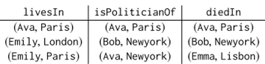
Table 1 presents a small knowledge base that is used as a running example to illustrate the important concepts.
2.1
Representation
Table 1: Example KB.
livesIn isPoliticianOf diedIn
(Ava,Paris) (Ava,Paris) (Ava,Paris) (Emily,London) (Bob,Newyork) (Bob,Newyork)
(Emily,Paris) (Ava,Newyork) (Emma,Lisbon)
We will use a KB representation based on a subset of first-order logic. Aconstant(e.g.,Emily) refers to a specific entity in the do-main and starts with an uppercase letter.Variables(e.g.,x) range over entities in the domain and are denoted by lowercase letters. Apredicateor relationR/n, wherenis the arity, represents a re-lationship among entities in the domain. In this paper, we only consider binary or arity two predicates, and will refer to the first argument as thesubjectand the second argument as theobject. A binary atomis of the formR(t1,t2), where each oft1andt2may
be either a constant or a variable. Aliteralis an atom or its negation. Aground atomis an atom where botht1andt2are constants. A
ground atom can be either true or false. A true ground atom is called afact. For the KB in Table 1, an example of a ground fact is
livesIn(Emily,London). For a given KBK, we use KRto refer to
the set of all ground facts for relationRthat appear inK. We use XRandYRto denote the set of constants that appear as a subject
or object in relationRinK, and they are defined as follows: XR = {x|∃y:R(x,y) ∈KR}, (2)
YR = {y|∃x:R(x,y) ∈KR}. (3)
A Datalogrulecan be written as an implicationB⇒H. The body
B, consists of a conjunction of literals, whereas the headHis a single literal. The following are examples of rules:
livesIn(x,y) ⇒diedIn(x,y), (4)
livesIn(x,y) ⇒isPoliticianOf(x,y), (5)
isPoliticianOf(x,y) ∧diedIn(x,y) ⇒livesIn(x,y). (6) A rule isgroundedorinstantiatedif all variables have been re-placed by constants. An instantiation of Rule (6) is
diedIn(Ava,Paris) ∧isPoliticianOf(Ava,Paris)
⇒livesIn(Ava,Paris) (7) The head of an instantiated rule is apredictionif all the literals in the rule’s body appear in K. In our running example,
livesIn(Ava,Paris)is a prediction becausediedIn(Ava,Paris) andisPoliticianOf(Ava,Paris)both appear in the KB shown in Table 1. The symbolPB⇒Hdenotes the set of predictions made by a
ruleB⇒Hwhen applied to the facts in a knowledge baseK.
2.2
Evaluation Metrics for Rules
Many metrics exist to evaluate the quality of a rule. Two of the most common ones are support and confidence.
A rule’ssupportorcoverageis defined as the number of predic-tions made by the rule that appear in a given KBK:
supp(B⇒R)=|KPB⇒R|=|PB⇒R∩KR|. (8)
where KPB⇒Rrepresents the set of “known positive” (KP)
exam-ples, that is, the predictions that already appear inK. Galarraga et al. [12] prefer this definition as it is monotonically decreasing, which enables applying many standard pruning techniques that can substantially improve the run time efficiency of rule learning. A rule’sconfidenceor precision is defined as the proportion of its predictions that are correct. However, KBs that are automatically populated from Web usually only contain facts (i.e., ground atoms that are true) and are open world, meaning that the truth value of any ground atom not in the KB is unknown. Therefore, ifPB⇒R
contains any ground atoms that are not in the KB, the confidence cannot be computed. One standard approach to this problem is to make a closed-world assumption (CWA) and assume that all ground atoms not in the KB are false. This yields the following definition:
ConfCWA(B⇒R)=
supp(B⇒R) |PB⇒R|
. (9)
Clearly, the CWA is false when KBs are automatically populated from the Web, and hence using it is suboptimal.
Galarraga et al. [12] addressed this by proposing the partial completeness assumption (PCA), which assumes that if we know oneyfor a givenxandR, that is,R(x,y) ∈KR, we know all theys
for thatxandR. Effectively, this allows them to infer the following set of negative examples for a KBK:
INR={R(x,y′) |R(x,y′)<KR∧y′∈YR∧∃y:R(x,y) ∈KR}
These negative examples can be used to compute a rule’s confidence, yielding the definition:
ConfPCA(B⇒R)=
supp(B⇒R)
supp(B⇒R)+|INR∩PB⇒R|
. (10)
The PCA assumption is suitable for relations that act like functions and have at most one object for every subject (e.g.diedIn), pre-suming the knowledge base is accurate. However, the assumption may be violated whenever a relation may associate multiple objects with each subject. Most relations fall into this category. In this case, its viability will solely depend on how complete the knowledge base is. Another potential weakness is that the PCA Confidence ignores the number of the predictions made by the rule.
2.3
Rule Generation
Approaches for generating first-order definite clauses have been ex-tensively studied in the inductive logic programming literature [19]. Our goal is not to revisit how rules are constructed; we are simply modifying the score function used to evaluate the quality of each rule. Hence, we make use of the highly efficient rule generation strategy employed in the AMIE+ system [12]. The implementation employs a variety of techniques from the database community to achieve good scalability. At a high level, it generates rules as fol-lows: As input, the user provides a support threshold and maximum clause length. The algorithm maintains a queue of rules, which ini-tially contains one rule for each relation with an empty body (i.e., ⇒R). Rules are removed from the queue and refined by adding literals to the body according to a language bias that defines legal
rules (e.g., maximum length, etc.). It then checks the support of the refined rule, and if it exceeds the support threshold, the rule is returned. Furthermore, the modified rule is added to the queue for possible further refinement.
3
RC CONFIDENCE SCORE
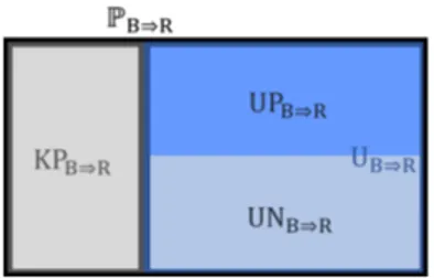
We propose a novel confidence score for evaluating rules in open-world problems. From a learning and evaluation perspective, each prediction made by an individual ruleB⇒Reither falls in the set of known positive examples KPB⇒R(that is, it appears in the given knowledge baseK) or belongs to a set UB⇒Rof unlabeled examples
(that is, it does not appear inK). Any ground atom not inKcould either be true or false. Thus, conceptually, these unlabeled examples can be subdivided into two sets
Unknown positives This is the set of ground atoms that are true but do not appear inK. They are denoted by UPB⇒R.
Unknown negatives This is the set of the ground atoms that are false and do not appear inK. They are denoted by UNB⇒R.
Figure 1 illustrates this subdivision of the predictions.
Figure 1: The set of predictionsPB⇒Rcan be divided into
la-beled (KPB⇒R) and unlabeled (UB⇒R) examples. Furthermore,
UB⇒Rcan be subdivided into the unknown positives (UPB⇒R)
and unknown negatives (UNB⇒R).
Based on the above division, a rule’s confidence could then be calculated as:
supp(B⇒R)+|UPB⇒R|
|PB⇒R|
(11) Our insight is that estimating a rule’s confidence only requires knowing the size of the set UPB⇒R. That is, computing a confidence
score does not require knowing precisely which ground atoms that do not appear in the knowledge baseKare true, just how many of them are true. Thus, computing the confidence of a rule reduces to estimating the size of this set.
We propose a novel way to estimate the size of UPB⇒R that
only relies on information available in the KB and subsequently incorporate it when evaluating rules. There are two key questions we need to address to estimate this set size, which are:
(1) What is the relationship between the proportion of known and unknown positives covered by a rule?We address this by making the relationship between coverage assumption, which is outlined in Subsection 3.1.
(2) What percentage of the unlabeled data for a given re-lation is expected to be positive?We begin in Subsection 3.2 by discussing two ways to compute this quantity, which we refer to asβ. However, in Subsection 3.3 we detail several
subtleties that we must contend with when usingβto arrive at the final estimate for the number of unknown positives.
3.1
Relationship between Coverage
Assumption
Our key assumption is that the proportion of positive examples covered by a rule is the same for both the labeled and unlabeled ex-amples. We call this the relationship between coverage assumption (rc), and it is defined as follows:
rc(B⇒R)=supp(B⇒R) |KR| =
|UPB⇒R|
|UPR|
, (12)
where UPRrepresents the set of all true facts for relationRthat do
not appear in the KBK. Intuitively, this would hold if the instanti-ations ofRthat appear inKwere selected completely at random from the set of all true facts forR.2
Our goal is to estimate the size of UPB⇒R, which we could do
if we knowrc(B⇒R)and|UPR|. Computingrcis straightforward.
Computing|UPR|is trickier.
3.2
Determining
β
We useβto denote the proportion of all the unlabeled examples that belong to the positive class. This true value ofβ, which is unknown, is:
β= |UPR|
|UR|
, (13)
where URrepresents the set of all facts for relationRthat do not
appear inK. Now we discuss several options for estimating this proportion.
One obvious solution for estimatingβis to randomly sample a number of groundings forR, check which ones are true and use this to estimateβ. This would likely entail significant work, as manual labels would need to be acquired for each relation. Thus, we propose two different, data-driven ways to estimateβthat only rely on information guaranteed to be available in the KB (e.g., do not rely on the availability of type constraints).
One possibility is to estimateβby making the partial complete-ness assumption. This yields the following definition:
βPCA= |KR|
|XR| × |YR|
, (14)
However, this is likely to be an overestimate in many cases. Con-sider, the relationisPoliticianOf. Relatively speaking, there are very few people who are politicians. Using Equation 14 will assume politicians represent the entire set of people, and will therefore overestimate the proportion of the overall population who are politicians.
Thus, a better possibility is to defineβon a per-rule basis as:
βB⇒R=
supp(B⇒R) |XB⇒R| × |YB⇒R|
, (15)
whereXB⇒RandYB⇒Rare defined as:
XB⇒R = {x|∃y:R(x,y) ∈PB⇒R}, (16)
YB⇒R = {y|∃x:R(x,y) ∈PB⇒R}. (17)
Settingβin this way considers a larger set of constants (without relying on type constraints) and hence avoids the aforementioned drawback ofβPCA.
3.3
Computing
|
UP
R|
Our goal is to only use information that is guaranteed to be available to compute|UPR|. Therefore, we do not wish to use type constraints,
as they may be unknown. Thus, a first thought for computing|UPR|
is to consider the number of instantiations ofRthat are not in the KB that could be constructed using the observed constants inPB⇒R.
Then we could multiply this number byβ, leading to the following calculation:
|UPR|=β× |{R(x,y) |x∈XB⇒R,y∈YB⇒R} \KR|. (18)
However, Equation (18) ignores the subtlety that each relation behaves differently in terms of the number of objects we would expect to be associated with each subject and vice versa. For exam-ple, thebornInrelation is a function because each person is only born in one city. However, a person can have multiple nationalities, although we would expect this number to be bounded by a small constant. To see how this issue affects computing|UPR|, consider
partitioning UB⇒Rinto the following four subsets:
XoldYold = {R(x,y) |x∈ (XB⇒R∩XR), y∈ (YB⇒R∩YR)}, XoldYnew = {R(x,y) |x∈ (XB⇒R∩XR), y∈ (YB⇒R\YR)}, XnewYold = {R(x,y) |x∈ (XB⇒R\XR), y∈ (YB⇒R∩YR)}, XnewYnew = {R(x,y) |x∈ (XB⇒R\XR), y∈ (YB⇒R\YR)}.
For example, ifRonly associates one object with each subject (i.e., it is a function), then all the new predictions (i.e., those not in the KB) that fall intoXoldYoldandXoldYnew will be false.
Therefore, we need to estimate the number of unknown positives separately for each subset. The two trickiest subsets areXoldYnew andXnewYold, as we need to scale back the estimated number of positives examples in these subsets. To see why, considerXoldYnew. Here, we need to account for the fact that each subject already ap-pears inKRwith some objects, so we would expect it to associate
with fewer new objects (on average) than if the subject did not appear inKR. We do this by considering forXoldYnew (XnewYold) the proportion of possible new objects (new subjects) that are as-sociated with each old subject (old object). This is captured by the functionality and inverse functionality of a relation [12]. We use a slight modification from past work [12],3and definefX(R)and fY(R)as: fX(R) = 1−HMx∈XR 1 |{y|R(x,y) ∈K|} (19) fY(R) = 1−HMy∈YR 1 |{x|R(x,y) ∈K|} (20) where HM is the harmonic mean. The functions return a value between zero and one. The value of fX(R) (fY(R)) is zero if the
relation is a function (inverse function).
Finally, like the PCA, we ignoreXoldYoldand assume that all of these predictions are false. We use this data to compute the information needed to derive the size of UPB⇒R, so any estimates
3The only change is inserting the1−in front of the harmonic mean, which we do simplify the notation later on.
on this subsample of the data will likely be overly optimistic. We estimate the unknown positives for the remaining three subsets as: |UPXol dYnew| = |XoldYnew| ×βB⇒R×fX(R) ×rc(B⇒R),
|UPXnewYol d| = |XnewYold| ×βB⇒R×fY(R) ×rc(B⇒R),
|UPXnewYnew| = |XnewYnew| ×βB⇒R×rc(B⇒R).
3.4
The Final RC Metric
This leads to our rule confidence score, which for a ruler:B⇒R
is defined as:
ConfRC(r)=
supp(r)+|UPXol dYnew|+|UPXnewYol d|+|UPXnewYnew|
|Pr| . (21)
3.5
Comparing Different Evaluation Measures
To illustrate the differences between the CWA, PCA, and RC, we will use our KB from Table 1 and Rule (5):r: livesIn(x,y) ⇒isPoliticianOf(x,y).
This rule produces three predictions:isPoliticianOf(Ava,Paris),
isPoliticianOf(Emily,London)andisPoliticianOf(Emily,
Paris). Only one of these appears in the KB. Hence, the
supp(livesIn(x,y) ⇒ isPoliticianOf(x,y)) = 1. Now, let us consider the various confidence scores for this rule.
CWA.BecauseisPoliticianOf(Emily,London)and
isPoliticianOf(Emily,Paris)do not appear in the KB in Table 1, the CWA means that these are assumed not to be true. Thus, the confidence with this assumption is:
ConfCW A(r)= 1
3=0.33 (22)
PCA.The PCA assumption would assume thatAvaandBobare not politicians in any other city. However, becauseEmilydoes not appear in theisPoliticianOfrelation, it assumes nothing about whetherEmilyis a politician. Because the PCA does not produce any negative examples that are in the prediction set, the PCA confidence measure is:
ConfPCA(r)= 1
1+0 =1 (23)
The PCA Confidence for this rule is 1.0, even though clearly not every resident of a city is also a politician in that city.
RC.When calculating theRCconfidence we would like to esti-mate how many of the remaining 2 unlabeled predictions are also positive. TheXr has two elements (Ava,Emily) andYr has as well two elements (Paris,London) and therefore the estimate of the proportion of groundings that are true is:
βr = 1 2×2 =
1
4 (24)
Next, we divideUr into 4 subsets:
XoldYold ={(Ava,Paris)},
XoldYnew ={(Ava,London)},
XnewYold ={(Emily,Paris)},
The calculation must also take into account the relation’s properties, where fX(isPoliticianOf)=1−2 3 = 1 3 (25)
shows that a person can be a politician in different cities. Similarly we also calculatefY(isPoliticianOf)=13. Using the definition of
thercassumption we calculate the relationship to be:
rc(r)= supp(r) |KisPoliticianOf| =
1
3, (26)
In the next step, we calculate the estimated number of positives in each of the subsets:
|U PXol dYnew|=1× 1 4× 1 3× 1 3 = 1 36, (27) |U PXnewYol d|=1×1 4× 1 3× 1 3 = 1 36, (28) |U PXnewYnew|=1× 1 4× 1 3= 1 12. (29)
Finally, we can compute the confidence measure for the rule:
ConfRC(r)=
1+(361 +361 +121)
3 =0.38 (30)
4
EMPIRICAL EVALUATION
We will evaluate our proposed confidence metric in the context of inferring novel facts to include in a KB. Specifically, our goal is to address the following questions:
(1) When using the AMIE+ system, does employing our pro-posed RC confidence score result in more accurate predic-tions than using the PCA confidence score?
(2) What is the effect of type constraints on the precision of the predictions?
(3) How well do the confidence measures estimate the precision of a rule?
(4) How doesβr compare toβPCA?
(5) How does the proposed approach compare to the Subgraph Feature Extraction approach (SFE) [13]?
In order to answer these five questions, we will compare the fol-lowing algorithms:
RC + types: RC confidence usingβB⇒Rand RDF type
con-straints
PCA + types: PCA confidence and RDF type constraints RC: RC confidence usingβB⇒Rand no type constraints
PCA: PCA confidence and no type constraints
RC_PCA + types: RC confidence usingβPCAand RDF type constraints
4.1
Methodology
We used the AMIE+ [12] system to learn rules (see Sect. 2.3) on the YAGO2 [16] and Wikidata KBs. We employed the same parameter settings from the original paper and setminHC = 0.01(support threshold) andmaxLen = 3, which resulted in 137 and 1515 learned rules, respectively. After finding all rules that meet the support threshold, the AMIE+ system only retains those that also satisfy a threshold on the PCA confidence, which we set to 0.1 for the YAGO2 KB as in the AMIE+ paper. Consequently, the final rule set for the YAGO2 KB consisted of the 69 rules from the initial 137 that
met this threshold. As far more rules met the support threshold in the Wikidata KB, we employed a higher PCA confidence threshold of 0.6, which resulted in 456 rules from the initial set of 1515 being selected.
When using our proposed confidence score, it would also be nat-ural only to consider those rules that meet both a support threshold and a threshold on the RC confidence score. However, when compar-ing the PCA and RC confidences, we want to avoid any differences in performance arising due to the fact that each confidence score led to a different number of rules being selected. Therefore, in order to ensure a fair comparison between the two confidence metrics, instead of using a threshold on the RC confidence, we selected rules using it as follows. We ordered the list of rules that met the support threshold (137 for YAGO2 and 1515 for Wikidata) according to the RC confidence metric. Then, we selected the top 69 rules for the YAGO2 KB and top 456 rules on the Wikidata KB according the RC confidence. Hence, the rule sets selected using each confidence score contain different rules in them, but are of the same size.
Using the selected rules, we generated all predictions and as-signed a confidence to each prediction. As some predictions can be derived from multiple, different rules, we calculated the confidence score for each ground atom using Galarraga et al.’s method [12]:
score(R(x,y))=1− n
Ö
i=1
(1−Conf∗(ri)), (31) whereri,i∈ {1, . . . ,n}is the set of rules that predictR(x,y)and
Conf∗is the appropriate confidence measure. This formula assigns
a higher confidence value to ground atoms derived from multi-ple rules, which intuitively makes sense. In the cases where we consider type constraints, we used therdf:typeconstraints from the YAGO3 KB [22], type constraints for Wikidata properties, and type-checking NELL constraints. In this case, any prediction that violates the constraints is discarded.
To evaluate the quality of the predictions, we generated a single ranking over all relations based onscore(R(x,y)). Based on the con-fidence scores, we divided the predictions into buckets of width 0.01 (e.g., the first bucket contains the predictions with scores between 1 and 0.99, the second bucket contains the predictions with scores between 0.99 and 0.98, etc.). We calculated the precision for the first bucket such that, cumulatively, 10 thousand predictions were made. Then, we evaluated every subsequent bucket such that an additional 50 thousand predictions were made. Then, like Galarraga et al. [12], we estimated the cumulative precision, by randomly sampling 100 unlabeled predictions from any bucket which repre-sents a range of confidence scores that are equal to or higher than the current bucket. For predictions on the YAGO2 KB, we checked if each selected prediction appeared in the YAGO3 KB, and if so we labeled it as correct. If it did not appear in the YAGO3 KB, we manually checked the fact. We manually labeled all selected facts on the Wikidata KB.
To compare our approach with the Subgraph Feature Extraction approach (SFE) [13], we used the NELL KB [5]. SFE, which is an enhancement of the Path Ranking Algorithm (PRA) [17], learns a separate model for each relation, and generates predictions sepa-rately for each relation. We used the same data as used in Gardner and Mitchell [13] and Gardner et al. [14], which focuses on the
10 relations in the NELL KB with the largest number of known instances. We obtained the set of predictions for all 10 relations using the SFE algorithm and placed them into buckets based on the SFE probability measure [14]. We also ran the AMIE+ system on the NELL data using the same support threshold as previously mentioned. Then, we only kept the 139 rules that had one of the 10 considered relations as the head. We ranked all rules according to both the PCA and RC confidences, and employed the previously procedure to make predictions with each rule set.
The characteristics for the YAGO2, Wikidata, and the used subset of the NELL KBs are provided in Table 2.
Table 2: Characteristics of each knowledge base considered in the experimental evaluation.
KB # facts # relations YAGO2 948K 33 Wikidata 8.4M 430 NELL 3.4M 520
4.2
Results
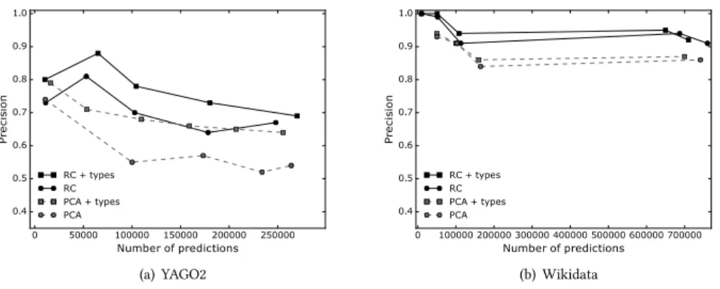
4.2.1 RC vs. PCA Confidence.To address the first question, we compare the rule sets selected using the RC and PCA confidences with and without type constraints on the YAGO2 and Wikidata KBs. Figure 2 shows the precision for all approaches. The RC con-fidence achieves a superior precision regardless of the number of predictions made and regardless of the KB. At the beginning, when only a few predictions are made, both approaches perform simi-larly. However, larger differences begin to emerge as more facts are predicted.
We will now discuss the results on the YAGO2 KB in more detail. The precision when using the RC confidence increases after the first point in the plot. This metric ranks the rule
isMarriedTo(x,y) ∧hasChild(x,z) ⇒hasChild(y,z) first. While this rule is logical and relevant, the YAGO2 KB is fairly complete with respect to thehasChildrelations. Hence, this rule ends up making a number of predictions that describe the stepchild relation, which leads to slightly lower precision at the top of the ranked list of predictions.
The precision when using the PCA confidence decreases as more predictions are made. This metric ranks the following rules second and third:
diedIn(x,y) ∧isLocatedIn(y,z) ⇒isPoliticianOf(x,y)
livesIn(x,y) ∧isLocatedIn(y,z) ⇒isPoliticianOf(x,z).
Generally speaking, these rules do not hold and hence create a large number of highly ranked, yet incorrect predictions.
4.2.2 Effect of Type Constraints. As expected, Figure 2 shows that including type constraints improves performance for both metrics. However, using the RC confidence without type constraints results in equivalent or slightly better performance than PCA with type constraints on the YAGO2 KB and better performance on the Wikidata KB. Furthermore, the RC confidence without type constraints is better than PCA without type constraints. These
results give additional evidence that reasoning about the unlabeled data in a more sophisticated manner, as the RC confidence measure does, can be beneficial.
4.2.3 Rule-by-rule comparison. We selected nine rules learned on YAGO2 KB and compared the PCA and RC (both with type con-straints) confidences to the confidence of the rule as estimated on manually labeled data. The chosen rules are ranked highly accord-ing to at least one of the score functions or reflect the differences between them. We estimated the confidence by randomly sam-pling 100 predictions for each rule. Predictions that appeared in the YAGO3 KB were labeled as correct and the others were assessed manually.
The results are presented in Table 3. For each rule, the table gives both the PCA and RC confidence measures and the rule’s rank among all learned rules. It also includes the number of predictions made by each rule that did not appear in the KB (i.e., the size of UB⇒R) and the precision as estimated on the manually labeled data.
The RC confidence tends to systematically underestimate the precision of rules. Perhaps this occurs becauseβB⇒Ris an
under-estimate of the true proportion of the true facts in the unlabeled data. When estimating the precision using the RC confidence, we divide the set of unlabeled predictions into subsets based on the previous appearance of subjects and objects in the KB. The RC con-fidence tends to rank rules where one (or more) of those subsets is empty, higher. Empty subsets can arise whenfX(R)andfY(R)equal
zero. Considering the characteristics of each relation allows the RC confidence to perform better. The RC confidence also tends to rank rules that make fewer predictions that fall outside the KB higher.
In contrast, the PCA confidence over- or under-estimates the precision based on the characteristics of the rule. For example, when calculating the confidence for a relation that has many objects for each subject (e.g.,dealsWith), the PCA confidence tends to underestimate the precision. Its estimates of the precision tend to be better when a subject has close to (or exactly) one object for each subject.
While the confidence estimates may not be well calibrated, they do tend to produce good rankings. There is an extensive literature on calibrating estimates via post processing (e.g. [6, 33]), and it would be possible to adapt these techniques to our setting.
4.2.4 Comparing Differentβs.Figure 3 shows a comparison be-tween usingβB⇒RandβPCAon the YAGO2 KB. Clearly, usingβB⇒R
results in better performance. The primary issue with usingβPCA is that it tends to way overestimate the confidence in several cases. Namely, it struggles when the relation in the rule head contains one argument where only a small subset of the entities that could appear in that argument position will appear in a true ground atom that involves that the relation, such as the following rule:
livesIn(x,y) ∧isLocatedIn(y,z) ⇒isPoliticianOf(x,z).
4.2.5 Comparison to SFE..Finally, we compare AMIE+ with both the PCA and RC confidence measures to the Subgraph Fea-ture Extraction (SFE) approach [13], which is recent, well-known approach to KB completion. Figure 4 shows a comparison between the SFE algorithm and AMIE+ using the PCA and RC confidence on the described subset of the NELL KB. SFE achieves the highest
(a) YAGO2 (b) Wikidata
Figure 2: Comparing the effect of using type constraints on the precision of the predictions as a function of the number of predictions made for both the RC and PCA confidence measures.
Table 3: For nine rules learned on the YAGO2 KB, we report the PCA and RC confidence scores (together with each rule’s rank) as well as an estimate of the rule’s true precision.|UB⇒R|reports the number of predictions that are unlabeled.
PCA RC
Rule |UB⇒R| Conf Rank Conf Rank Precision
isMarriedTo(x,y) ⇒isMarriedTo(y,x) 5635 0.92 1 0.59 2 1.00
diedIn(x,y) ∧isLocatedIn(y,z) ⇒isPoliticianOf(x,z) 13038 0.85 2 0.03 67 0.36
created(x,y) ∧produced(x,y) ⇒directed(x,y) 1018 0.59 8 0.50 5 0.13
isMarriedTo(x,y) ∧hasChild(x,z) ⇒hasChild(y,z) 2643 0.58 9 0.59 1 0.51
bornIn(x,y) ∧isLocatedIn(y,z) ⇒isPoliticianOf(x,z) 33559 0.57 11 0.01 83 0.33
hasChild(x,y) ∧hasChild(z,y) ⇒isMarriedTo(x,z) 1971 0.41 20 0.50 4 0.86
livesIn(x,y) ⇒isPoliticianOf(x,y) 14515 0.29 32 0.01 85 0.29
dealsWith(x,y) ∧dealsWith(y,z) ⇒dealsWith(x,z) 1121 0.28 33 0.29 8 0.94
dealsWith(x,y) ⇒dealsWith(y,x) 595 0.18 47 0.15 17 1.00
Figure 3: The effect of usingβB⇒R versusβPCA on the RC
confidence measure on the YAGO2 KB. The plot shows the precision of the predictions as a function of the number of predictions made.
performance when only a very small number of predictions are made, however, its performance quickly degrades. After around 1500 predictions, the rules learned by AMIE+ regardless of which confidence measure is used perform much better. Furthermore, the RC confidence measure again outperforms the PCA confidence.
Figure 4: Comparison of the RC, PCA and SFE approaches on the considered subset of the NELL KB. The plot shows the precision of the predictions as a function of the number of predictions made.
5
RELATED WORK
We now discuss how our work is related to learning definite clauses, KB completion, and learning from positive and unlabeled data (PU Learning).
Learning Definite Clauses.Inductive logic programming (ILP) [19] is the standard approach for learning definite clauses. Typical ILP systems require both positive and negative examples to evaluate the score of an individual rule. However, there have been several attempts to define score functions based only on positive examples and no unlabeled data. Muggleton [24] and the LIME system [23] developed an approach that is based on a Bayesian estimate. Ef-fectively, these approaches work by randomly generating some negative examples. The SHERLOCK system [28] employs a score function based on statistical relevance and statistical significance to identify interesting rules. We differ from this approach in that we explicitly attempt to make use of the unlabeled data.
Knowledge Base Completion.There are many approaches to infer additional facts to include in a KB [14, 15, 18, 25, 31, 32]. One set of approaches [14, 18] work by using ideas from ILP and relational learning to convert the KB into a graph. Then, they con-struct features based on paths in the graph and build one classifier (e.g., logistic regression) per relation. Another set of approaches use matrix factorization to obtain new relations. Either by putting positive facts into the rows of a matrix, and inference rules into the columns [32] or by putting relations into rows and entity pairs into the columns of the matrix [15], these systems, using scalable matrix factorization approaches, learn new facts to complete KBs. Recently, there has been interest in neural network approaches [25, 29, 31] to this problem. These approaches encode entities in a vector represen-tation and attempt to predict if a given relation holds for a pair of input entities. One of these approaches [29] works in an open-world setting, but requires a text corpus to do so. A primary advantage to learning rules over the neural network based approaches is that the rules are easy for humans to interpret, can give an explana-tion for why a predicexplana-tion was made, and represent new knowledge themselves.
PU LearningOur work is clearly related to the field of learning from positive and unlabeled data [8, 10, 21, 26]. In this setting, a learner only has access to positive examples and a (large) set of unlabeled data. The assumption is that the unlabeled data contains both positive and negative examples. This paper differs from past work in three important ways. One, we propose a method for es-timating the fraction of unlabeled examples that belongs to the positive class. Two, we define a novel score function based on this proportion and the behavior of the target relation. Three, we focus on relational data, whereas the other work on PU learning that we are aware of work on propositional data.
The idea for the relationship between coverage assumption (that is, the computation ofrcin Equation 12), is similar in spirit to the technique employed by Denis et al. [8] for decision tree learning and Ritter et al. [26] for logistic regression and Naïve Bayes. However, these works assumeβwas given. Several approaches (e.g., [2, 9, 10] propose methods for estimating this quantity, but from proposi-tional data. One of these methods [3] was recently extended to the relational setting, but only focused on predicting unary predicates. Ritter et al. [27] introduce penalties in the relation extraction ap-proach for missing data in the text and KB. They estimate penalties based on the assumption that extractions for popular entities are more likely to be negative than those involving rare entities.
6
CONCLUSIONS AND FUTURE WORK
In this paper, we have proposed a new confidence measure to rank first-order rules learned from an open-world KB. Taking inspiration from the learning from positive and unlabeled data setting, our metric attempts to incorporate information about the unlabeled data into our metric. Our key insight is that we only need to reason about number of “positive” examples that are not in the KB. We discussed several factors that must be accounted for when estimating this number and our approach requires no additional information apart from what is in the KB. Empirically, our metric results in a better ranking than the state-of-the-art PCA metric. Furthermore, our proposed approach performs better than SFE, which is another well-known approach for KB completion. In the future, we will explore different ways to estimateβ, as well as other ways to reduce the consistent underestimate of our confidence measure. Additionally, we believe our metric is generally applicable and could be used to evaluate rules learned from an open-world KBs using other rule learners such as Aleph or FOIL and would like to investigate this. Finally, we want to evaluate our metric using additional KBs.
ACKNOWLEDGMENTS
We would like to thank Jessa Bekker, Hendrik Blockeel and the anonymous reviewers for their very helpful feedback on this pa-per. JD is partially supported by the KU Leuven Research Fund (C14/17/070, C22/15/015, C32/17/036) and FWO-Vlaanderen (G.0356.12, SBO-150033).
REFERENCES
[1] Sören Auer, Christian Bizer, Georgi Kobilarov, Jens Lehmann, Richard Cyganiak, and Zachary Ives. 2007. DBpedia: A nucleus for a Web of open data.The Semantic Web4825 (2007), 722–735.
[2] Jessa Bekker and Jesse Davis. 2018. Estimating the class prior in positive and unlabeled data through decision tree induction. InProceedings of the 32nd AAAI Conference on Artificial Intelligence.
[3] Jessa Bekker and Jesse Davis. 2018. Positive and unlabeled relational classifica-tion through label frequency estimaclassifica-tion. InProceedings of the 27th International Conference on Inductive Logic Programming (ILP).
[4] Kurt Bollacker, Colin Evans, Praveen Paritosh, Tim Sturge, and Jamie Taylor. 2008. Freebase: a collaboratively created graph database for structuring human knowledge. InProceedings of the 2008 ACM SIGMOD international conference on Management of data. Vancouver, Canada, 1247–1250.
[5] Andrew Carlson, Justin Betteridge, and Bryan Kisiel. 2010. Toward an Architec-ture for Never-Ending Language Learning.. InProceedings of the 24th Conference on Artificial Intelligence (AAAI’10). 1306–1313. https://doi.org/10.1002/ajp.20927 [6] Rich Caruana and Alexandru Niculescu-Mizil. 2006. An empirical comparison of supervised learning algorithms. InProceedings of the 23rd international conference on Machine learning (ICML’06). 161–168.
[7] Luc De Raedt, Anton Dries, Ingo Thon, Guy Van den Broeck, and Mathias Verbeke. 2015. Inducing Probabilistic Relational Rules from Probabilistic Examples.. In
IJCAI. 1835–1843.
[8] François Denis, Rémi Gilleron, and Fabien Letouzey. 2005. Learning from positive and unlabeled examples.Theor. Comput. Sci.348, 1 (2005), 70–83. https://doi.org/ 10.1016/j.tcs.2005.09.007
[9] Marthinus Christoffel du Plessis, Gang Niu, and Masashi Sugiyama. 2017. Class-prior estimation for learning from positive and unlabeled data.Machine Learning
106, 4 (2017), 463–492.
[10] C. Elkan and K. Noto. 2008. Learning Classifiers from Only Positive and Unla-beled Data. InProceedings of the 14th ACM SIGKDD International Conference on Knowledge Discovery and Data Mining (KDD 2008). 213–220.
[11] D. Foxvog. 2010. Cyc. InTheory and Applications of Ontology: Computer Applica-tions(1 ed.), Roberto Poli, Michael Healy, and Kameas Achilles (Eds.). Springer Netherlands, 259–278.
[12] Luis Galárraga, Christina Teflioudi, Katja Hose, and Fabian M Suchanek. 2015. Fast Rule Mining in Ontological Knowledge Bases with AMIE +. The VLDB Journal24, 6 (2015), 707–730.
[13] Matt Gardner and Tom Mitchell. 2015. Efficient and Expressive Knowledge Base Completion Using Subgraph Feature Extraction. InProceedings of EMNLP’15.
1488–1498. https://doi.org/10.1016/j.artint.2016.09.003
[14] Matt Gardner, Partha Talukdar, Jayant Krishnamurthy, and Tom Mitchell. 2014. Incorporating vector space similarity in random walk inference over knowledge bases. InProceedings of EMNLP.
[15] Wenqiang He, Yansong Feng, Lei Zou, and Dongyan Zhao. 2015. Knowledge Base Completion Using Matrix Factorization. InWeb Technologies and Applications -17th Asia-PacificWeb Conference (APWeb’15). 768–780.
[16] Johannes Hoffart, Fabian M. Suchanek, Klaus Berberich, and Gerhard Weikum. 2013. YAGO2: A spatially and temporally enhanced knowledge base from Wikipedia.Artificial Intelligence194, Artificial Intelligence, Wikipedia and Semi-Structured Resources (2013), 28–61. https://doi.org/10.1016/j.artint.2012.06.001 [17] Ni Lao, Tom Mitchell, and William W Cohen. 2011. Random walk inference and learning in a large scale knowledge base. InProceedings of the Conference on Empirical Methods in Natural Language Processing. Association for Computational Linguistics, 529–539.
[18] Ni Lao, Amarnag Subramanya, Fernando Pereira, and William W Cohen. 2012. Reading the web with learned syntactic-semantic inference rules. InProceedings of the 2012 Joint Conference on Empirical Methods in Natural Language Processing and Computational Natural Language Learning. Association for Computational Linguistics, 1017–1026.
[19] N. Lavrac and S. Dzeroski (Eds.). 2001.Relational Data Mining. Springer-Verlag, Berlin.
[20] Dekang Lin and Patrick Pantel. 2001. DIRT@ SBT@ discovery of inference rules from text. InProceedings of the seventh ACM SIGKDD international conference on Knowledge discovery and data mining. ACM, 323–328.
[21] Bing Liu, Yang Dai, Xiaoli Li, Wee Sun Lee, and Philip S. Yu. 2003. Building Text Classifiers Using Positive and Unlabeled Examples. InProceedings of the Third IEEE International Conference on Data Mining (ICDM ’03). IEEE Computer Society, Washington, DC, USA, 179–.
[22] Farzaneh Mahdisoltani, Joanna Biega, and Fabian M Suchanek. 2015. YAGO3 : A Knowledge Base from Multilingual Wikipedias. InProceedings of the Conference on Innovative Data Systems Research, CIDR ’15.
[23] Eric McCreath and Arun Sharma. 1997. ILP with Noise and Fixed Example Size: A Bayesian Approach. InProceedings of the Fifteenth International Joint Conference on Artifical Intelligence. Morgan Kaufmann Publishers Inc., San Francisco, CA, USA, 1310–1315.
[24] Stephen Muggleton. 1997. Learning from Positive Data. InSelected Papers from the 6th International Conference on Inductive Logic Programming (ILP ’96). Springer-Verlag, London, UK, UK, 358–376.
[25] Arvind Neelakantan, Benjamin Roth, and Andrew McCallum. 2015. Composi-tional vector space models for knowledge base completion. InProceedings of the Annual Meeting of the Association for Computational Linguistics.
[26] Alan Ritter, Evan Wright, William Casey, and Tom Mitchell. 2015. Weakly Supervised Extraction of Computer Security Events from Twitter. InThe 24th ACM International World Wide Web Conference (WWW’15). 896–905. https: //doi.org/10.1145/2736277.2741083
[27] Alan Ritter, Luke Zettlemoyer, Mausam, and Oren Etzioni. 2013. Modeling Missing Data in Distant Supervision for Information Extraction.Transactions of the Association for Computational Linguistics1 (2013), 367–37.
[28] Stefan Schoenmackers, Oren Etzioni, Daniel S Weld, and Jesse Davis. 2010. Learn-ing first-order horn clauses from web text. InProceedings of the 2010 Conference on Empirical Methods in Natural Language Processing. Association for Computational Linguistics, 1088–1098.
[29] Baoxu Shi and Tim Weninger. 2018. Open-World Knowledge Graph Completion. InProceedings of 32nd AAAI Conference on Artificial Intelligence.
[30] Amit Singhal. 2012. Introducing the Knowledge Graph: things, not strings. (2012). [31] Richard Socher, Danqi Chen, Christopher D Manning, and Andrew Ng. 2013.
Rea-soning with neural tensor networks for knowledge base completion. InAdvances in neural information processing systems. 926–934.
[32] William Yang Wang and William W Cohen. 2016. Learning First-Order Logic Embeddings via Matrix Factorization. InProceedings of the 25th International Joint Conference on Artificial Intelligence (IJCAI’16). 2132–2138.
[33] Bianca Zadrozny and Charles Elkan. 2001. Obtaining calibrated probability estimates from decision trees and naive Bayesian classifiers. InProceedings of the Eighteenth International Conference on Machine Learning (ICML’01). 609–616.