New Architectures for Very Deep Learning
Doctoral Dissertation submitted to the
Faculty of Informatics of the Università della Svizzera Italiana in partial fulfillment of the requirements for the degree of
Doctor of Philosophy
presented by
Rupesh Kumar Srivastava
under the supervision of
Jürgen Schmidhuber
Dissertation Committee
Antonio Carzaniga Università della Svizzera Italiana, Switzerland Michael Bronstein Università della Svizzera Italiana, Switzerland Ruslan Salakhutdinov Carnegie Mellon University, USA
Sepp Hochreiter Johannes Kepler Universität Linz, Austria
Dissertation accepted on 1 February 2018
Research Advisor PhD Program Director Jürgen Schmidhuber Walter Binder
I certify that except where due acknowledgement has been given, the work presented in this thesis is that of the author alone; the work has not been submit-ted previously, in whole or in part, to qualify for any other academic award; and the content of the thesis is the result of work which has been carried out since the official commencement date of the approved research program.
Rupesh Kumar Srivastava Lugano, 1 February 2018
Dedicated to Govind Lal Srivastava
We can only learn what we already almost know.
Patrick Winston
Abstract
Artificial Neural Networks are increasingly being used in complex real-world applications because many-layered (i.e., deep) architectures can now be trained on large quantities of data. However, training even deeper, and therefore more powerful networks, has hit a barrier due to fundamental limitations in the design of existing networks. This thesis develops new architectures that, for the first time, allow very deep networks to be optimized efficiently and reliably. Specifically, it addresses two key issues that hamper credit assignment in neural networks: cross-pattern interferenceandvanishing gradients.
Cross-pattern interference leads to oscillations of the network’s weights that make training inefficient. The proposed Local Winner-Take-All networks reduce interference among computation units in the same layer through local competi-tion. An in-depth analysis of locally competitive networks provides generalizable insights and reveals unifying properties that improve credit assignment.
As network depth increases, vanishing gradients make a network’s outputs increasingly insensitive to the weights close to the inputs, causing the failure of gradient-based training. To overcome this limitation, the proposed Highway networks regulate information flow across layers through additional skip con-nections which are modulated by learned computation units. Their beneficial properties are extended to the sequential domain with Recurrent Highway Net-works that gain from increased depth and learn complex sequential transitions without requiring more parameters.
Acknowledgements
I would like to thank my supervisor Jürgen Schmidhuber for the opportunity to conduct this research, and for the countless discussions that helped me understand how to think about artificial intelligence. A special thanks also goes to Faustino Gomez, who encouraged and supported me continuously throughout my PhD.
I am very grateful to my co-authors Jonathan Masci, Julian Zilly, Klaus Greff, Marijn Stollenga and Sohrob Kazerounian for our fruitful research collaborations. Together with the rest of IDSIA members, they gave me a fun and stimulating work environment for several years. In particular, I must thank Cinzia Daldini, who helped me in every official matter I was ever involved in during my PhD. I’m also grateful to Jianfeng Gao, Li Deng and Xiaodong He, who gave me the opportunity to spend an incredibly stimulating summer at Microsoft Research in Redmond.
Thanks to Bas Steunebrink, Faustino Gomez, Jan Koutník and Wonmin Byeon for reading and suggesting improvements to drafts of this thesis, and to my dissertation committee members – Antonio Carzaniga, Michael Bronstein, Ruslan Salakhutdinov and Sepp Hochreiter – for taking the time to review my work. Finally, I am forever grateful to my family for their love and support in pursuing this journey.
Contents
Contents xi
List of Figures xv
List of Tables xvii
List of Acronyms xix
1 Introduction 1
1.1 Motivation . . . 1
1.2 Contributions . . . 3
1.3 Overview . . . 4
2 Background 7 2.1 The Credit Assignment Problem . . . 7
2.2 Supervised Learning . . . 8
2.2.1 Maximum Likelihood Estimation . . . 9
2.2.2 Underfitting & Overfitting . . . 10
2.3 Neural Networks . . . 11
2.3.1 Types of Networks & Layers . . . 12
2.3.2 Output Activation Functions . . . 14
2.4 Training Neural Networks . . . 15
2.4.1 Objective Functions . . . 15
2.4.2 Regularization . . . 15
2.4.3 Backpropagation . . . 16
2.4.4 Gradient Descent . . . 17
3 Challenges & Related Work 19 3.1 The Trainability Gap . . . 20
3.1.1 Cross-pattern Interference & Competitive Learning . . . 20
xii Contents
3.1.2 Step Size Adaptation . . . 21
3.1.3 Initialization Strategies . . . 22
3.1.4 Activation Functions . . . 23
3.1.5 The Challenges of Depth . . . 23
3.1.6 Techniques for Training Very Deep Networks . . . 25
3.2 The Generalization Gap . . . 27
4 Local Winner-Take-All Networks 29 4.1 Networks with Local Winner-Take-All Blocks . . . 30
4.2 Comparison with Related Methods . . . 32
4.2.1 Max-pooling & Maxout . . . 32
4.2.2 Dropout . . . 33
4.2.3 Rectified Linear Units . . . 33
4.3 Experiments . . . 34
4.3.1 Permutation Invariant MNIST . . . 36
4.3.2 CNNs on MNIST . . . 36
4.3.3 Amazon Sentiment Analysis . . . 37
4.4 Analysis of Subnetworks . . . 38
4.5 Implicit Long Term Memory . . . 39
4.6 Discussion . . . 40
5 Understanding Locally Competitive Networks 43 5.1 Locally Competitive Networks . . . 43
5.2 Hypothesis . . . 44
5.3 Subnetwork Analysis . . . 46
5.3.1 Visualization through Dimensionality Reduction . . . 46
5.3.2 Behavior during Training . . . 48
5.3.3 Evaluating Submasks . . . 49
5.3.4 Effect of Dropout . . . 51
5.4 Experiments on Larger Datasets . . . 53
5.4.1 CIFAR-10 & CIFAR-100 . . . 53
5.4.2 ImageNet . . . 53
5.5 What about Sigmoidal Networks? . . . 55
5.6 Discussion . . . 56
6 Highway Networks 59 6.1 Architecture . . . 59
6.2 Variants of Highway Networks . . . 61
xiii Contents
6.3.1 Setup . . . 63
6.3.2 Optimization Stress Test . . . 64
6.3.3 MNIST Digit Classification . . . 65
6.3.4 Comparison to Fitnets on CIFAR-10 . . . 65
6.3.5 Results on CIFAR-10 and CIFAR-100 . . . 66
6.4 Analysis . . . 67
6.4.1 Routing of Information . . . 68
6.4.2 Layer Importance . . . 69
6.5 Comparison of Highway Network Variants . . . 70
6.5.1 Image Classification . . . 71
6.5.2 Language Modeling . . . 74
6.6 Discussion . . . 75
7 Recurrent Highway Networks 77 7.1 Recurrence Depth in RNNs . . . 77
7.2 Architecture . . . 79
7.3 Experiments . . . 80
7.3.1 Optimization Stress Test . . . 82
7.3.2 Sequence Modeling . . . 85
7.4 Analysis . . . 87
7.5 Discussion . . . 88
8 Conclusion 91 8.1 Future Work . . . 92
Publications during the PhD program 95
Figures
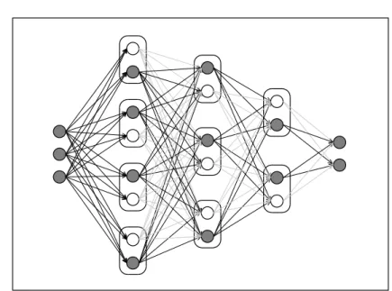
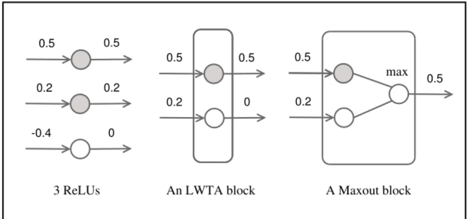
4.1 Illustration of a Local Winner-Take-All (LWTA) network. . . 30
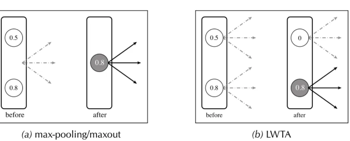
4.2 Max-pooling/maxout vs. LWTA. . . 32
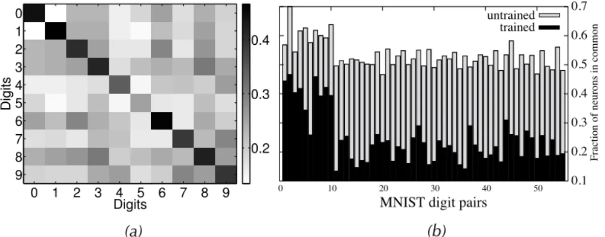
4.3 Analysis of subnetworks in LWTA networks. . . 38
5.1 Comparison between ReL, LWTA and maxout . . . 44
5.2 Illustration of subnetworks within a ReL network. . . 45
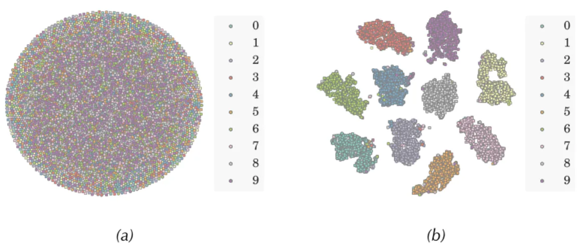
5.3 2-D Visualization of submasks from a ReL network for MNIST. . . 47
5.4 2-D Visualization of submasks from untrained networks for MNIST. 48 5.5 2-D Visualization of submasks from trained LWTA and maxout networks for MNIST. . . 49
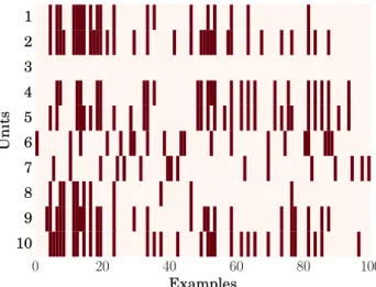
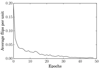
5.6 Progression of unitflipsduring network training. . . 50
5.7 2-D Visualization of submasks from trained maxout networks for CIFAR-10 and CIFAR-100. . . 52
5.8 Submask-based image retrieval on the ImageNet 2012 dataset. . . 56
5.9 Sample retrieval results on the ImageNet 2012 dataset. . . 57
6.1 Comparison of optimization of plain networks and Highway net-works of various depths. . . 63
6.2 Inspection of the learned biases, gate outputs and block outputs for trained Highway networks. . . 68
6.3 Visualization of activations and biases of trained Highway networks. 69 6.4 Layer lesioning experiment for Highway networks trained on MNIST and CIFAR-100. . . 70
6.5 Comparing 50-layer Highway vs. Residual networks on ImageNet 2012 classification. . . 72
7.1 Illustration of the importance of recurrence depth in RNNs. . . 79
7.2 Schematic illustration of a Recurrent Highway Network layer. . . . 81 7.3 Optimization experiment results for Recurrent Highway Networks. 82 7.4 Word-level language modeling results on Penn Treebank using RHNs. 83
xvi Figures
7.5 Mean activations of the transform gates at different depths in a trained RHN. . . 88 7.6 Lesioning results for RHN. . . 89
Tables
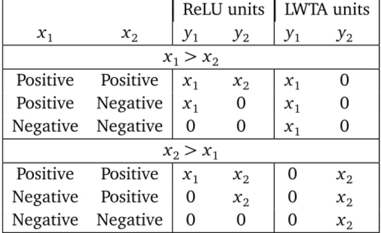
4.1 Comparison of rectified linear activation and LWTA. . . 34
4.2 Performance of LWTA networks on permutation invariant MNIST classification. . . 35
4.3 Performance of CNNs with LWTA on MNIST classification. . . 37
4.4 Local competition guards against catastrophic forgetting. . . 39
5.1 Results for MNIST digit recognition using submasks. . . 51
5.2 Classification errors on CIFAR datasets comparing maxout network performance,kNN on activation values,kNN on pre-activations. . 54
5.3 Comparison of Top-5 classification accuracy obtained using sub-masks from different CNNs on ImageNet 2012. . . 54
5.4 Comparison of submasks and Diffhash binary codes on the Ima-geNet 2012 dataset. . . 55
6.1 Results for MNIST digit classification with Highway networks. . . 62
6.2 Experimental comparison betweenFitnetsand Highway networks for CIFAR-10 object recognition. . . 65
6.3 Results for CIFAR-10 and CIFAR-100 object recognition with High-way networks. . . 67
6.4 Comparison between Highway network variants trained for Ima-geNet 2012 object recognition. . . 71
6.5 Comparison of various Highway variants for character-aware neu-ral language models. . . 74
7.1 Results for Penn Treebank word-level language modeling with RHNs. 84 7.2 Results forenwik8symbolic sequence modeling with RHNs. . . 86
7.3 Results fortext8symbolic sequence modeling with RHNs. . . 86
Acronyms
AI Artificial IntelligenceCNN Convolutional Neural Network FNN Feedforward Neural Network LCN Locally Competitive Networks LSTM Long Short-Term Memory LWTA Local Winner-Take-All MLP Multilayer Perceptron NN Neural Network
ReL Rectified Linear
RHN Recurrent Highway Network RNN Recurrent Neural Network WT Weight Tying
WTA Winner-Take-All
Chapter 1
Introduction
1.1
Motivation
The objective of building powerful computing machines is to program them to perform tasks that are too complex, time-consuming, expensive, dangerous or repetitive to be performed by humans. Many of these tasks require machines to exhibit intelligent behavior typically shown by animals, such as perception, reasoning or planning. For example, a computer programmed as a telemedicine agent is required to understand a patient’s health condition through a series of questions and answers, and then suggest an appropriate course of action. To take another example, a robot may be required to assist in disaster relief efforts by planning the rescue of an affected population.
Broadly, there are two ways to program machines to exhibit desired behavior (i.e., produce certain outputs in response to certain inputs) within the limits of computer science[Gödel, 1931]. The first is to manually program the computer to produce the behavior based on expert knowledge, which has been the com-mon approach in the design of many control systems. However, for many tasks sufficient expert knowledge is unavailable or incomplete. An example of this is in the field of computer vision where decades of research into hand-designed image processing algorithms has not resulted in high-performing general object recognition[Russakovsky et al., 2015]. Even if expert domain knowledge is avail-able, writing programs for all of the large number of tasks humans are interested in is likely to take prohibitive amounts of time and effort. So the first approach is attractive for certain narrowly-defined tasks, but not a satisfactory long-term solution. The second approach is to define a specification that can be used to test the desired behavior, and then run a search procedure in the space of programs. The advantage of this program searchapproach is that it is very general, with
2 1.1 Motivation
the primary disadvantage being that the search may take too long to succeed in practice.
It was recognized early on that program search can be substantially sped up if, like intelligent animals, machines can use examples of correct behavior or experiences to guide the search for desired programs. The primary hurdle in obtaining these speedups is thecredit assignment problem[Newell, 1955; Samuel, 1959; Minsky, 1961]. In order for a machine to improve its own behavior by learning from experience – what is calledmachine learning– it is necessary for it to properly attribute its successes and failures to its past decisions such that it can apply the appropriate changes.
Artificial neural networks (henceforth referred to as NNs or simply “networks”) are a biologically inspired class of mathematical models used to implement pro-grams in machine learning[Deng and Chen, 2014; Schmidhuber, 2015; Goodfel-low et al., 2016]. They consist of a set of simple interconnected processing units, usually organized in groups called layers, which can in principle approximate arbitrary functions [Cybenko, 1989; Hornik et al., 1989]and run arbitrary pro-grams[Siegelmann and Sontag, 1995]. Crucially, if the functions implemented by the processing units are differentiable, there exists an efficient procedure for credit assignment in arbitrary NNs: backpropagation [Linnainmaa, 1970, 1976; Werbos, 1981]. This algorithm computes the gradients of a network’s outputs with respect its parameters efficiently, allowing gradient-based search techniques to be used for learning.
In recent years, this property combined with two key enabling factors has generated wide interest in NNs, in particular for perception problems[LeCun et al., 2015; Schmidhuber, 2015; Malik, 2017], although they have been studied since the 1960s. The first of these enablers is the abundance of labeled data, fueled by the ubiquity of the Internet and dedicated efforts to curate and label datasets for the purposes of machine learning. The second is availability of increasingly large amounts of computational power, which is required to learn from large datasets with high variability and complexity, or complicated simulations of physical systems.
Unfortunately, as more complex learning tasks are targeted, success of NNs is hampered by several difficulties in training them. In particular, the efficiency of gradient-based learning is highly dependent on the design of the neural network, i.e., its architecture. Credit assignment using backpropagation in increasingly large and complex networks becomes more and more difficult, and gradient based training algorithms face a multitude of obstacles such as plateaus, saddle points, and local minima. The number of layers in the network, the number of computation units in each layer, the non-linear functions implemented by
3 1.2 Contributions
the units, and their connectivity all play crucial roles in determining how fast the network can be trained in practice or if the training succeeds at all. These choices also affect generalization, i.e., performance on unseen input data, since an architecture with a more suitable inductive bias[Mitchell, 1980]will result in better generalization for certain problems.
A particularly critical issue in NNs is that as the number of layers connected in a chain (itsdepth) increases, credit assignment through backpropagation becomes increasingly difficult or even altogether infeasible[Hochreiter et al., 2001]. This is an important limitation since it is well known that increasing the number of layers is an efficient way to increase the potential complexity of functions that can be modeled using NNs[Bengio et al., 2013]. Many recent empirical breakthroughs in supervised machine learning have been achieved using large and deep NNs. Network depth played perhaps the most important role in these successes. For instance, within just a few years, the top-5 image classification accuracy on the 1000-class ImageNet dataset increased from ∼84% [Krizhevsky et al., 2012] to ∼95% [Szegedy et al., 2014; Simonyan and Zisserman, 2014]using deeper networks with rather small receptive fields per layer[Ciresan et al., 2011, 2012]. Similar trends in other domains such as speech recognition have also underscored the superiority of deeper networks in terms of accuracy and/or efficiency[Yu et al., 2013; Zeiler et al., 2013]. Therefore, network architectures that improve credit assignment and have suitable inductive biases for practical problems can improve and scale the application of machine learning methods across a variety of domains, from perception to modeling, control and decision-making.
Based on these motivations, the central motivation for this thesis isto develop neural network architectures that permit efficient and reliable training of large and deep neural networks. To this end, we design network architectures that improve credit assignment among computation units in the same layer through local competition, and across multiple layers through additional connections in the network which are modulated by learned computation units.
1.2
Contributions
In order to achieve our goals, we address two key issues that hamper credit assignment in neural networks: cross-pattern interference [Sutton, 1986] and vanishing gradients[Hochreiter et al., 2001].
First, we propose a new architecture based on local competition called Local Winner-Take-All (LWTA). In this architecture, units in a layer are arranged in groups, and competition among units in each group prevents interference between
4 1.3 Overview
learning signals from multiple training patterns. LWTA networks match or exceed the performance of other network types in supervised learning experiments, and they also have a reduced tendency to forget previously learned tasks when abruptly trained on a new task.
Next, we explore a unifying interpretation of LWTA together with recently popular rectified linear [Jarrett et al., 2009] and maxout [Goodfellow et al., 2013b]networks as a collection of an exponential number of linear subnetworks. Several experiments are performed to understand the extent and utility of this interpretation: visualization of the active subnetworks, their training behavior, suitability of subnetwork identities for classification, and impact of training with dropout. The results confirm that implicit gating of input patterns based on their mutual similarity plays a key role in the success of the three network types.
A main limitation of the above developments is that local competition improves shallow NNs but not deep ones. In particular, NNs with more than about 20 layers still remain very hard to train, suggesting that competition between units improves credit assignment among units in each layer, but not across several layers. To address the vanishing gradient problem that causes this, we combine insights from LWTA and Long Short-Term Memory[Hochreiter and Schmidhuber, 1997b]. The resulting Highway network architecture overcomes the challenge of training very deep networks reliably and produces state-of-the-art results on the CIFAR-100 benchmark. When training a very deep network on two different tasks, we show that a Highway network automatically learns to utilize more layers for the “harder” task that intuitively requires more computational resources. Comparative experiments are used to demonstrate how variants of Highway networks can lead to similar or different results depending on the task.
Finally, we propose Recurrent Highway Networks (RHNs), which use Highway layers to extend and improve LSTM networks. They address another unsolved challenge related to depth: training recurrent neural networks with large depths in the recurrent transition function which maps previous states to new states during sequence processing. Using RHNs, we obtain increasingly improved results for progressively deeper networks with constant number of parameters, and set a new state of the art on the challenging enwik8 and text8 benchmarks for modeling text sequences from Wikipedia.
1.3
Overview
The rest of the thesis is organized as follows: Chapter 2 introduces basic concepts and establishes the relevant background for the rest of the thesis. Chapter 3
5 1.3 Overview
identifies the key difficulties that prevent the effective use of NNs for machine learning. It also provides a summary of past work that has attempted to address these difficulties. Chapter 4 introduces Local Winner-Take-All LWTA networks, a new architecture that utilizes local competition and guards against cross-pattern interference. Chapter 5 presents a unifying analysis of three different locally competitive architectures, including LWTA networks, and demonstrates the extent of their conceptual similarities. Chapter 6 develops the Highway network archi-tecture that makes reliable training of very deep networks possible and evaluates its performance on several image classification datasets. Chapter 7 extends the Highway architecture to the sequential setting resulting in Recurrent Highway Networks. Profiting from their increased recurrence depth, Recurrent Highway Networks outperform the state-of-the-art on two challenging sequence modeling benchmarks. Finally Chapter 8 closes the thesis with a summary of the proposed architectures and a discussion of promising directions for future work.
Chapter 2
Background
This chapter reviews the basic concepts that underlie the use of NNs for machine learning. The methods developed in this thesis are studied in the context of supervised machine learning, so the treatment is limited to this setting. More detailed exposition can be found in various textbooks on the subject [Bishop, 2006; Murphy, 2012; Goodfellow et al., 2016].
2.1
The Credit Assignment Problem
The desire to speed up search for programs brought up the credit assignment problem early on in research on Artificial Intelligence (AI). This was one of the challenges that Newell [1955]; Samuel[1959]; Minsky[1961]and others identified in the context of developing programs to play games such as checkers and chess. These games were used as a proxy for understanding how a computer can successfully solve complex sequential decision making problems similar to humans. It was realized that it is particularly difficult to write expert programs for such problems, and so a learning system that could automatically design such programs would be necessary. Such a system would immediately face the credit assignment problem: if a machine makes several decisions to arrive at a result – say dozens of moves in a game of chess – how to know which decisions should have been different (and how) to obtain a better result? If this can not be known, any search for solution programs for complex problems involving a large number of intermediate decisions is unlikely to succeed in reasonable time. A method of measuring the impact of intermediate decisions (or outputs) of the program on the final outcome can direct the search towards better programs, leading to fast learning. For example, Newell[1955]suggested to break problems into subgoals, which would then provide additional signals for reinforcing useful decisions.
8 2.2 Supervised Learning
The credit assignment problem of sequential decision making is also relevant to the learning of static functions mapping inputs to outputs. In order to learn desired functions, a machine needs to identify which aspects of the data are important and to what extent. For example, a chess-playing machine might identify board configurations that are good or bad by selecting certain aspects of the configuration asfeatureson which further computations are performed. It is this capability of learning methods that gives them an edge over hand-designed programs which may lack the features crucial for obtaining good results. If one considers a learning method that produces internal representations of the data during a multi-step computation of the output, then these representations act like intermediate decisions similar to chess moves. This challenge is related to the problem of new terms [Samuel, 1959; Dietterich et al., 1982], and is nowadays referred to as the problem of representation learning [Bengio et al., 2013]. Assigning appropriate credit to internal representations can substantially speed up learning and make it practical[Rumelhart et al., 1986].
Some researchers explicitly distinguish between two subproblems of the credit assignment problem [Sutton, 1984]: thetemporalversion, where appropriate credit for a final outcomes should be assigned to earlier decisions, and the struc-turalversion, where credit for a final outcome should be assigned to participating computing units. The techniques developed in this thesis primarily attempt to improve structural credit assignment. In certain cases, as done in Chapter 7, the same techniques can be used to aid in temporal credit assignment.
2.2
Supervised Learning
In this thesis, techniques for improving credit assignment are developed in the context ofsupervisedlearning problems, in particular the setting of single-label classification [Bishop, 2006]. We are given a training setS of independently and identically distributed (i.i.d.) pairs of input patterns and targets(x,y)for training. “Supervised” refers to the availability of targets for guiding the training. Each input patternxis a real-valued vector associated with a single class label y ∈ {0, 1, . . . , K−1}where K is the total number of classes. The objective is to learn aclassifier: a functionF(x)that maps the inputs to class labels such that the classification error rate(CER) or a relatedobjective functionis minimized for atest setof input-target pairs. The test setS0is sampled from the same distribution as the training set, and does not contain elements in common with the training set.
9 2.2 Supervised Learning
The CER is defined as
CER(F,S0) = Σ
(x,y)∈S0 ¨
0 if(F(x) = y),
1 otherwise. (2.1)
Another problem setting, investigated in Chapter 7, which can be formulated as a supervised classification problem is that of modeling discrete sequences. These are sequential prediction problems such as predicting the next character or word in a natural language text or the next set of music symbols in a piano roll. Although the raw training data available in these cases are only samples of sequences, input-target pairs can be constructed by time-delaying input sequences to produce targets. For example, for the problem of word-level language modeling, training datasets are prepared by using words from raw sentences as input sequences, and the same word sequences shifted by one time step as target sequences. Once the data is prepared in this form, the methods for supervised classification are used to learn functions that predict the next symbol in the sequence at each time step. The main differences from the classification setting are that:
• The class of functions used for learning is different, capable of processing and producing sequential data.
• The learned function are interpreted and used asgenerativemodels of the data, rather than discriminative classifiers. Such models can be used for generating new samples from the data distribution, or for biasing/evaluating the outputs of another model.
2.2.1
Maximum Likelihood Estimation
A principled approach for supervised classification that results in a consistent training and evaluation methodology is to train probabilistic classifiers using maximum likelihood estimation (MLE)[Bishop, 2006; Murphy, 2012]. Assume that functionF(x)maps input patterns to probabilitiesp(Ck|x),k∈ {0, 1, . . . , K−1}
instead of classes. F is represented with a (sufficiently powerful) model such as an NN with a set of adjustable parameters arranged in a vectorθ. The desired values of the parameters are fixed but unknown. The probability assigned by the classifier to the target class is p(y|x,θ). The class prediction for computing the
CER is taken to be the label with the highest assigned probability arg max k
p(Ck|x). The likelihood function L(θ) is defined as the probability assigned by the classifier to all samples in the training set for a given θ. Since the training samples are i.i.d.,
10 2.2 Supervised Learning
L(θ) =p(S |θ) = Y
(x,y)∈S
p(y|x,θ). (2.2)
Maximum likelihood training involves estimating the value of the parameters for which the likelihood is maximized:
θMLE=arg max
θ
L(θ). (2.3)
Intuitively, maximizing the likelihood of correctly classifying the training set also minimizes the CER. It is common practice to minimize the negative log of the likelihood instead, giving
θMLE=arg min
θ
X
(x,y)∈S
−logp(y|x,θ). (2.4)
This does not change the results since log is a monotonically increasing func-tion, but is done for multiple reasons: it increases the stability of computations, it is more compatible with optimization literature which often considers minimiza-tion instead of maximizaminimiza-tion problems, and it closely relates the quantity being minimized to those used in training approaches other than MLE.
2.2.2
Underfitting & Overfitting
MLE casts learning as a specific optimization (or search) problem. One can define a modelF, the search space forθ, and then invoke a suitable optimization algorithm for minimizing the objective function. This may not always succeed: the obtained model may fail to produce low error rate on the training set. This can happen because the selected model is not powerful enough to capture all the information in the data for accurate prediction, or because the optimization procedure fails to exploit its full expressive power – a phenomenon termedunderfitting. Underfitting can be addressed by using models that can learn more complex functions, but care must be taken since complex models can be more difficult to optimize.
On the other hand, successfully obtaining a low error rate on the training set may still result in poor performance on unseen data from the test set. This happens due to overfitting – the model’s expressive power allows it to rely on unique properties of the randomly selected training samples instead of learning properties that can generalize to unseen test samples. Overfitting and underfitting are challenges faced in almost every learning task and combating these issues is a large and active field of study[Burnham and Anderson, 2003].
11 2.3 Neural Networks
In supervised machine learning, overfitting is often controlled through model regularization. It refers to techniques for encouraging simpler model configura-tions over complex ones, according to some notion of simplicity, in accordance with Occam’s razor[Pearl, 1978; Angluin and Smith, 1983; Blumer et al., 1987]. The simplest regularization method is to add an additional termλR(θ)to the maximum likelihood objective function, whereλis a weighting factor andRis a regularization function of the model parameters. Most common regularization functions have a Bayesian interpretation as priors over the model parameters. For example, setting λR(θ) =θ>θ (called L2 weight decay) corresponds to
as-suming that the prior distribution of the model parameters is Gaussian[Bishop, 2006]. Some regularization techniques commonly used with NNs are discussed in subsection 2.4.2.
2.3
Neural Networks
NNs are used as models for a variety of machine learning problems, whether they be in supervised, unsupervised or reinforcement learning[Bishop, 2006; Sutton and Barto, 1998]. Some early models that can be characterized as types of NNs (e.g. Perceptrons[Rosenblatt, 1958], Neocognitron[Fukushima, 1980b]) were inspired by models of information processing in the human brain, while others such as GMDH networks[Ivakhnenko, 1971]were motivated by data analysis and control problems. Modern NNs are descendants of these models, but depart significantly in design from their biological inspirations. Schmidhuber [2015] provides a detailed survey and historical overview of NN developments. In the rest of the chapter, we cover fundamental NN concepts relevant to the rest of the thesis. More details on all these topics can be found in books by Bishop[1995, 2006]; Graves[2012]; Goodfellow et al.[2016].
A wide variety of NNs exist, but in this thesis we will only consider deter-ministic networks trained in a supervised setting. An NN can be described as a computational graph of simple processing units (also called nodes or neurons) connected by weighted directed edges. Each unit computes some function of the inputs that it receives from units connected to it and emits the obtained outputs (called its activation). The set of units in the graph are often divided into subsets called layers; the number of units in a layer is referred to as its width. Subsets of units that receive inputs to the network are called input layers and subsets that produce network outputs are calledoutput layers. The termhidden layersis commonly used to refer to all other layers. The length of the longest path from the input to output layers is referred to as thedepth of the network.
12 2.3 Neural Networks
NNs with acyclic graphs are calledfeedforward NNsor FNNs, and those with cyclic graphsrecurrentNNs or RNNs. Unlike FNNs, RNNs contain connections that have time lags – they transfer outputs emitted by source units in the past to destination units (which may be the same as source units) at future time steps during processing of sequential inputs. In mathematical notation, it is often clearer to write NN equations in terms of computations at the layer level rather than the unit level thanks to the succinctness of matrix notation, so this convention is adopted throughout the thesis, except when noted otherwise.
FNNs with a single hidden layer are known to be universal approximators [Cybenko, 1989; Hornik et al., 1989], i.e., given enough hidden units, they can approximate any continous function up to any desired accuracy. Similarly, RNNs are known to be Turing-complete[Siegelmann and Sontag, 1995]in theory.
A series of results, starting from the work of[Håstad, 1987; Håstad and Gold-mann, 1991]for simple threshold circuits, and continuing to present day[Bengio et al., 2006; Bengio and Delalleau, 2011; Bianchini and Scarselli, 2014; Cohen et al., 2016]show that there are function classes which can be represented far more efficiently by deeper networks than shallower networks. In general, for most practical problems of interest, it is unknown if they fall in the above classes of functions. However, a pattern strong experimental results on challenging bench-marks in the domains of computer vision[Krizhevsky et al., 2012; Szegedy et al., 2014; Simonyan and Zisserman, 2014; He et al., 2016a]and speech recognition [Hinton et al., 2012a; Graves et al., 2013]indicates that this might be the case.
2.3.1
Types of Networks & Layers
Multilayer PerceptronThe simplest type of NNs consist of layers connected to form a linear graph. These networks are calledMultilayer Perceptrons(MLP)s, and they typically consist of fully-connectedlayers.
An MLP represents a functionF:Rm→Rn with L layers of computation units. The`th layer (`∈ {1, 2, . . . , L}) computes a non-linear transformation of its input x`and produces its outputˆy`. Since an MLP is a linear graph, the input to each layer is always the output of the previous layer, i.e.,x`=ˆy`−1. Thus,x1∈Rm is
the external input to the network andˆyL∈Rn is the network’s output. 1
The transformation implemented by a fully-connected layer involves first
1To keep notation intuitive, we useˆyto denote layer outputs andyto denote desired outputs
in this chapter. However, the desired output is not used in the rest of this thesis, so we simply use
13 2.3 Neural Networks
computing an affine functionz`of the input parameterized by weightsW`and bias b`, followed by application of a non-linear activation function f. To summarize:
x`=ˆy`−1 (2.5a)
z`=W`x`+b` (2.5b)
ˆ
y`= f(z`). (2.5c)
If layer`hasN`number of units, the dimensions ofW`areN`×N`−1 andb` is an N`-dimensional column vector. The set of all weights and biases is often collectively referred to as the parameters or weights of the network. Activation functions are typically unit-wise non-linearities such as thelogistic sigmoid(f(x) =
σ(x) = 1+1e−x) or the hyperbolic tangent (f(x) =tanh(x)), but in general they
can take other forms or incorporate their own learnable parameters.
The procedure of computing the output of a network given an input pattern is termed a forward pass. It is the sequential activation of all the layers in the network according to Equation 2.5 in topological ordering for a given input. In the case of an MLP,x1 is set to the given input vector and then layers 1, 2, . . . , L
are activated in order to computeˆyL. Fully Recurrent layer
There are many ways of adding time-lag connections to NNs, and as a result RNNs can have various topologies. See Lang et al.[1990]; Werbos[1990]; Elman [1990]for some early architectures. The simplest types of recurrent layer is called a fully recurrent layer or just, a simple RNN layer. Each unit in the layer has one-step time lag connections to all other units (called recurrent connections), and has incoming connections from all the inputs. As a result, the output of the layer at any time step tis a function of not just the inputs but also its output at the previous time step.
At any time step t>0 of sequence processing, letx[t]∈
Rm be the input to the RNN andyˆ[t]∈Rn be its output. ˆy[0]is typically set to be the zero vector, but in some cases it is set to another constant vector or learned during training. Let us denote byW∈Rn×m the matrix of connection weights from the inputs to the units, byb∈Rn a vector of bias weights and byR∈Rn×n the matrix of recurrent connection weights. The forward pass equations for a simple recurrent layer are:
z[t]=Wx[t]+Rˆy[t−1]+b (2.6a)
ˆ
14 2.3 Neural Networks
LSTM
The simple RNN layer described above is theoretically powerful, but ill-suited for gradient-based learning, as discussed in subsection 3.1.5. Due to this reason, the most successful recurrent architecture is Long Short-Term Memory (LSTM) [Hochreiter and Schmidhuber, 1997b], which was specifically designed to address the limitations of simple RNNs. The detailed architecture and its advantages are described in subsection 3.1.6.
Convolutional and Pooling layers
For data with spatial regularities such as images, the most popular choice of architecture used is a Convolutional Neural Network (CNN)[LeCun, 1989; LeCun et al., 1998]. Like an MLP, it is a linear graph of layers, with special layers that are designed to take advantage of the spatial relationships in the data. These layers are calledconvolutional layers, which apply a modification of the transformation used in fully-connected layers. In addition to convolutional layers, CNNs often utilizepoolingorsub-samplinglayers to reduce the spatial dimensionality of their inputs. Common types of pooling layers use themaxormeanoperations, applied over fixed size receptive fields of the inputs. Further details of these layers can be found in Goodfellow et al.[2016].
2.3.2
Output Activation Functions
The activation function used for the output layer of an NN depends on the interpretation of the outputs according to the problem. If the NN is being trained to predict unbounded real-valued targets, the identity activation f(x) = x is commonly used. Similarly, if the targets are bounded in the range [−1, 1], the tanhactivation function is a natural choice.
As discussed in section 2.2, the outputs of an NN trained as a probabilistic classifier or discrete sequential predictor are interpreted as a categorical probabil-ity distribution over the labels. To enable this, the activation f of the output layer of the NN must be changed such that the outputs always form a valid probability distribution. Thesoftmaxactivation function serves this purpose:
f(x) =softmax(x) = e x
15 2.4 Training Neural Networks
2.4
Training Neural Networks
2.4.1
Objective Functions
The forward pass is used to compute the outputs or predictions of a network for a given input. To train the network on a given dataset using the method discussed in section 2.2, an objective (also called the loss or error) function should be minimized, which measures the discrepancy between the networks predictions and the targets. Based on the MLE approach (Equation 2.4), the error function to be minimized in the supervised classification setting is
E(y,ˆyL) = X (x,y)∈S −logp(ˆy=y|x,θ) (2.8) = X (x,y)∈S −y>logˆyL, (2.9)
whereyis aone-hotvector encoding of the scalar target y as a binary vector with all elements equal to zero except the yth element which is set to one. For sequence prediction tasks, the error function is computed for each time step and then summed over the sequence length for each sequence.
2.4.2
Regularization
Apart from weight decay, three other commonly used NN regularization tech-niques are also used in this thesis. The particular choice of regularization for each experiment is primarily motivated by the need to ensure reasonably fair comparisons to recent work.
The first technique is to add random noise to the inputs, weights or activations of the network [Holmström and Koistinen, 1992; Bishop, 1995; Hinton et al., 2012b]. Dropout[Hinton et al., 2012b; Wan et al., 2013; Gal, 2015]is a modern and most effective variation of this technique which inserts multiplicative Bernoulli noise in the activations or weights of the network during training. For testing the network on a test set, the noise is removed and the weights are suitably scaled to account for the absence of noise.
The second technique is calledearly stopping[Holmström et al., 1989], and utilizes a held-outvalidation set(separate from the training and test sets) to detect overfitting during training. This is done by periodically monitoring a measure of performance (such as the CER) on both the training and validation sets during
16 2.4 Training Neural Networks
optimization, and stopping training when the training set performance continues to improve but the validation set performance starts to worsen.
Finally,batch normalization[Ioffe and Szegedy, 2015]is a recent technique which was introduced to improve the speed of gradient-based training of FNNs, but also acts as very effective regularization method in practice. Unlike the above two methods, this technique has not been widely adopted for preventing overfitting in RNNs.
2.4.3
Backpropagation
Backpropagation (often referred to asbackprop) is the most common method of assigning credit in NNs. It is an algorithm for efficiently computing derivatives of the outputs of a network with respect to its parameters. While earlier work had already used the algorithm for efficient computation of derivatives in NN-like functions[Linnainmaa, 1970; Dreyfus, 1973], it was the work of Werbos[1974, 1981]that first developed NN-specific backprop2. Interestingly, mirroring the con-text surrounding the first discussions of the credit assignment problem, backprop was also brought to NNs with the goal of training sequential decision making systems [Werbos, 2006]. Rumelhart et al. [1986]popularized backpropagation in the context of learning pattern recognizers by demonstrated that useful inter-nal representations emerged in NNs with hidden layers trained with the help of backprop. It was soon generalized for the case of RNNs[Robinson and Fallside, 1987; Werbos, 1988; Williams and Zipser, 1989]. Thus, backprop can be used to address both the structural and temporal credit assignment problems.
The procedure of applying backprop to compute derivatives of a network’s parameters is called abackward pass, since it involves going through the layers in the reverse order of the forward pass. During the backward pass, the derivatives with respect to each of the layer’s activations and parameters are computed with the help of activation values stored during the forward pass, and intermediate derivatives computed so far. This is the key feature of backprop – the complexity of the backward pass is the same as that of the forward pass.
The backward pass for the MLP described by Equation 2.5 proceeds as follows. First we define a useful quantityδ`for the layer`, called thedeltasfor the layer:
δ`:=∂
ˆ yL
∂z` (2.10)
The objective is to compute{∂yˆL ∂W`,
∂ˆyL
∂b`},`∈ {1, 2, . . . , L}. This can be done by
17 2.4 Training Neural Networks
starting at layer L and then using the following equations at each previous layer:
δL= f0(zL), (2.11a) δ`=W>`+1δ`+1·f0(z`), (2.11b) ∂ˆyL ∂W` =δ`x > `, (2.11c) ∂ˆyL ∂b` =δ`. (2.11d)
These equations can be used to compute the gradient of any loss function L of the network’s output with respect to its parameters using the chain rule:
∂L ∂W` = ∂L ∂yˆL ∂ˆyL ∂W` (2.12a) ∂L ∂b` = ∂L ∂yˆL ∂ˆyL ∂b` (2.12b) (2.12c) As long as the first term in the above products can be computed (simple if L is differentiable) or estimated, the second term can be computed using backprop.
When backprop is used for computing gradients for RNNs, it is termed Back-propagation Through Time (BPTT)[Werbos, 1990]. The main idea of the proce-dure is to unrollthe RNN: converting an RNN processing a sequence of T time steps into an FNN with T layers, where the same set of parameters are shared by all the layers. This is intuitively based on the similarity between Equation 2.6 for a simple RNN and Equation 2.5 for the MLP. The RNN equations can be transformed (unrolled) into the MLP equations by replacing time indices with layer indices, and adding a time-varying input at each layer in additional to the output of the previous layer. After unrolling, backprop as usual can be applied for efficient computation of gradients with respect to the RNN parameters with the same time complexity as the forward pass.
2.4.4
Gradient Descent
The simplest algorithm for optimizing an objective function when the gradient with respect to its parameters can be computed is gradient descent. It is an iterative algorithm, which at the nth iteration uses the gradient to apply an additive parameter update
18 2.4 Training Neural Networks
∆θ(n) =−α ∂L
∂θ(n) (2.13)
∆θ(n+1) =θ(n) +∆θ(n) (2.14) The learning rateαis ahyperparameter. Similar to other hyperparameters such as the topology of the network, the regularization weight etc., its value is typically selected from a set of values based on validation set performance.
It is well known that always changing parameters in the exact direction of steepest descent can be harmful, since the learning rate should be adapted dif-ferently for different parameters [Sutton, 1986]. It is common to use modified versions of gradient descent due to this reason. The most common variant incor-poratesmomentum[Polyak, 1964; Nesterov, 1983]which changes the parameter updates to
∆θ(n) =η∆θ(n−1)−α ∂L
∂θ(n) (2.15)
whereηis a hyperparameter. Momentum makes it easier for the optimization algorithm to avoid getting stuck due to local minima and other tricky properties of the objective function[Sutton, 1986; Rumelhart et al., 1986; Plaut et al., 1987; Jacobs, 1988].
A final modification to gradient descent which makes it practical for training on large training sets is the use of small subsets of the training set (calledbatches orminibatches) to compute approximate gradients, instead of the full gradient computed for the entire training set. Weights are updated after forward and backward passes for each batch, instead of waiting for the entire training set to be processed which might require prohibitive amounts of time and memory. When each batch consists of only one training pair, the resulting algorithm is called stochastic gradient descent. Although many other variations of gradient descent exist (see subsection 3.1.2 for some alternatives) batch gradient descent with momentum is used for all the experiments in this thesis. It is simple, easy to implement, works well in practice, and the choice ensures that improvements obtained in training with the proposed architectures are not due to use of a special optimization method.
Having discussed the central ideas for setting up and training NNs for super-vised learning, in the next chapter we discuss the issues arising in following these concepts and trying to apply NN-based learning methods to problems in prac-tice. This discussion will set up the stage for novel NN architectures introduced Chapter 4 onwards that are designed to address these issues.
Chapter 3
Challenges & Related Work
Based on the tools discussed in the previous chapter, the recipe for attacking a given problem using NNs is as follows: First, design an NN that is expected to have sufficient representational power for the task. Then choose an appropriate objective function based on a learning strategy (such as MLE) and techniques to prevent overfitting. Finally, select and run an optimization algorithm to train the network.1
Unfortunately, for a large number of problems the above procedure does not result in a network that performs acceptably well on the test set. Assuming that the amount of data available is sufficient and the objective function is appropriate for the task, the reasons for failure can be broadly categorized into the following issues:
a) Trainability gap: The optimization algorithm fails to sufficiently minimize the objective function on the training set (in terms of desired performance or available time budget), even though the NN is in principle capable of learning the task very accurately (a type of underfitting).
b) Generalization gap: The network obtained as a result of training performs much worse on the test set (unseen data) than the training set (overfitting). This chapter provides a discussion of these issues, and reviews important techniques from the literature that have been proposed to address them. Since the methods developed in this thesis are primarily motivated by the trainability gap, this issue is discussed in more detail. In particular, the problems arising from making NNs very deep are discussed, since as discussed earlier, depth is
1Due to the involvement of several hyperparameters in these steps, it is usually necessary to
run several trials and choose the best performing hyperparameter values.
20 3.1 The Trainability Gap
an important characteristic that makes them capable of modeling extremely complicated functions.
3.1
The Trainability Gap
In general training NNs is computationally intractable, i.e., there exist no efficient algorithms for training an arbitrary network on a arbitrary problem[Blum and Rivest, 1989; Judd, 1990; Hammer and Villmann, 2003]. There has been much research into understanding under which constraints the training of certain classes of NNs may be tractable[Anthony and Bartlett, 2009], but this quest is further complicated by the fact that a theoretical understanding and categorization of many practical problems of interest is missing. In practice, since there exists an efficient algorithm for computing gradients for arbitrary differentiable networks (backpropagation), most popular optimization algorithms for NNs are gradient-based, such as variants of steepest descent.
The ability to compute gradients efficiently is not a panacea. The objective function landscape for NNs is non-convex, with multiple local minima, saddle points and other characteristics that make optimization using gradient based methods tricky[Bishop, 1995]. These difficulties have motivated the development of a variety of techniques to improve and speed up the training of NNs which are discussed in this section. In the following chapters, new architectures are developed to specifically address two key issues that hamper credit assignment in NNs: cross-pattern interference (subsection 3.1.1) and vanishing gradients (subsection 3.1.5).
3.1.1
Cross-pattern Interference & Competitive Learning
Cross-pattern interference[Sutton, 1986]arises naturally in gradient-based train-ing of NNs when several units in the network simultaneously try to learn useful computations for a varied set of input patterns. This can make learning inefficient, since the weights of the units oscillate due to conflicting information coming from different patterns presented to the network over time, and these oscillations increase the total time required for the weights to converge.
A consequence of cross-pattern interference is catastrophic forgetting [ Mc-Closkey and Cohen, 1989; Carpenter and Grossberg, 1988], which is a funda-mental obstacle for the use of NN in continual learning systems[Ring, 1994]. In this setting, which is much more general than the supervised learning setting considered here, a machine’s goal is to continually improve its behavior over a
21 3.1 The Trainability Gap
single lifetime through interactions with its environement. Since the distribution of input patterns that the machine observes can change significantly over time, useful computations learned by an NN at earlier times get completely disrupted by new information, meaning that the machine can not profit from past experiences. Competitive Learning
Competitive interactions between units and neural circuits have long played an important role in biological models of brain processes. The effects of excitatory and inhibitory feedback found in many regions in the brain [Eccles et al., 1967; Anderson et al., 1969; Stefanis, 1969]were modeled with competitive interactions in several early models inspired by the brain’s information processing mecha-nisms[von der Malsburg, 1973; Grossberg, 1976; Fukushima, 1980a; Kohonen, 1982]. These demonstrations of successfully combining competitive interactions with simple Hebbian-like[Hebb, 1949]learning rules inspired further work by Rumelhart and Zipser[1985]for feature learning, and by Schmidhuber[1989] who used them in RNNs. However, these and several following developments of competitive learning since the 1990s[Ahalt et al., 1990; Goodhill and Barrow, 1994; Terman and Wang, 1995; Wang, 1997]did not use gradient-based training. The work of Jacobs et al.[1991a,b]was the first to leverage the properties of competitive interactions for the purpose of mitigating cross-pattern interference. They proposed to generalize competitive learning from the level of computational units to networks by employing a modular NN architecture. The architecture consisted of two types of networks, severalexpertnetworks and agatingnetwork. The output of the gating network was used to combine the outputs of the experts to produce the final network output. This explicit modularity of the architecture enabled it to avoid cross-pattern interference by allocating different input patterns to different experts. Related architectures were also developed by Pollack[1987] and Hampshire and Waibel[1992].
3.1.2
Step Size Adaptation
A common difficulty arising in NN optimization is that it may not be the best to always follow the exact steepest descent direction. This is due to the presence of structures like valleys and ravines in the landscape [Sutton, 1986; Jacobs, 1988; Qian, 1999]which require the use of different step sizes along different dimensions. This can be achieved with momentum – a widely employed technique to accelerate gradient descent[Polyak, 1964; Nesterov, 1983]that was brought to NNs in the 1980s[Rumelhart et al., 1986; Plaut et al., 1987; Jacobs, 1988].
22 3.1 The Trainability Gap
Another principled way to address the same issue is to use the inverse of the Hessian of the objective function to set the step sizes (i.e., Newton’s method), and incorporating information about the curvature of the function in addition to the gradient. Since this operation is computationally too demanding for all but the smallest networks, many researchers have proposed methods to compute and use approximations of the Hessian[Sutton, 1986; Becker and LeCun, 1988; Roux et al., 2008; Martens, 2010, 2014; Grosse and Salakhudinov, 2015].
Instead of computing the Hessian of the objective function for use with second order methods, another approach to speed up NN training is to still employ first order gradient descent algorithms but use certain “tricks” to encourage favorable properties of the Hessian. These tricks are choices regarding the network design, initialization and data preprocessing. For convex optimization, the convergence rate of gradient descent methods near the optimum is heavily influenced by the Hessian, in particular by itscondition number– the ratio of its largest and smallest eigenvalues – which should be close to unity for fast convergence. Some tricks for NN training that minimize the spread of eigenvalues are centering, normalizing and decorrelating the inputs[LeCun et al., 1998], using a scaled t anh activation function instead of the logistic sigmoid [LeCun et al., 1991; Kalman and Kwasny, 1992], and careful initialization of the weights[LeCun et al., 1998; Glorot and Bengio, 2010; He et al., 2015].
A related set of techniques attempt to make the non-diagonal terms of the Hessian as close to zero as possible [Schraudolph, 1998a; Raiko et al., 2012; Desjardins et al., 2015; Ioffe and Szegedy, 2015; Salimans and Kingma, 2016]. Doing so makes first order methods perform better since only the diagonal terms (one term corresponding to each dimension) need to be approximated. This can be accomplished with the help of variants of gradient descent which automatically adapt the step sizes per dimension. Popular choices include AdaGrad [Duchi et al., 2011], AdaDelta [Zeiler, 2012], RMSProp[Tieleman and Hinton, 2012] and Adam[Kingma and Ba, 2014].
3.1.3
Initialization Strategies
The initial values of a network’s weights have a direct impact on the success of optimization. One reason for this is that many activation functions are designed to saturatefor large magnitude inputs, so that the unit outputs are always bounded. Saturation refers to the fact that the output of the activation function changes negligibly as the input changes i.e. its gradient becomes almost zero. For example, for the t anh and hyperbolic sigmoid functions, large values of both positive and negative net input leads to saturation, which will impede gradient flow
23 3.1 The Trainability Gap
during the backward pass (subsection 2.4.3). In general, having too large or too small weights can severely attenuate signals (activations during forward pass, gradients during backward pass) as they propagate through a network. In conjunction with input data normalization[LeCun et al., 1991], normalized weight initialization techniques[LeCun et al., 1998; Glorot and Bengio, 2010; He et al., 2015]mentioned above are designed to make sure that the variance of the signals remains constant and close to one over the layers of the network. Of course, initialization can only guarantee favorable properties at the beginning of training, but practitioners have found that this is sufficient to enable successful training of small to medium-sized networks.
3.1.4
Activation Functions
In recent years, non-saturating activation functions have become popular, starting with the Rectified Linear (ReL)[Jarrett et al., 2009; Nair and Hinton, 2010; Glorot et al., 2011]function defined as y =max(0,x). Clearly this function does not saturate for positive inputs, and is therefore less likely to contribute to diminishing gradients during backpropagation. Moreover, while a complete theoretical under-standing of this phenomenon is currently lacking, it has been found that if the network weights are initialized according to normalization techniques mentioned above, the saturation behavior of ReL for negative inputs does not impede training if the network depth is not large. Following the popularity of ReL in applications, its variants that do not saturate for negative inputs either have also been tried [Maas et al., 2013; He et al., 2015]with mixed success.
In addition to preventing saturation, the activation function also affects opti-mization through its effect on the properties of the Hessian. The ReL function causes abias shiftat each layer because its output is always non-negative. Expo-nential Linear Units[Clevert et al., 2015]use a modification of ReL that addresses this issue and pushes the mean activations at each layer closer to zero, which improves the conditioning of the Hessian. Recent work has further built upon this to developself-normalizingnetworks[Klambauer et al., 2017]which preserve the mean and variance of signals during forward and backward propagation without requiring explicit normalization techniques.
3.1.5
The Challenges of Depth
The above issues contributing to the trainability gap are common to all NNs, but there is a specific challenge that fundamentally affects the trainability of powerful and efficient networks – gradient based training becomes increasingly infeasible
24 3.1 The Trainability Gap
as the depth of the credit assignment problem increases. It was first analyzed in the context of temporal credit assignment in RNNs[Hochreiter, 1991], and here we briefly review this analysis breifly.
Consider the simple RNN described in Equation 2.6. Ignoring the bias and inputs for clarity, the output of the RNN at time t isˆy[t]= f(Rˆy[t−1]). Then the temporal Jacobian At := ∂ˆy[t]
∂ˆy[t−1] is
At =diagf0(Rˆy[t−1])R. (3.1) Letγbe a maximal bound on f0 andσmax be the largest singular value ofR.
Then the norm of the temporal Jacobian satisfies
kAtk ≤diag
f0(Rˆy[t−1])kRk ≤γσmax (3.2)
As discussed in subsection 2.4.3, to compute thedelayedtemporal Jacobian of the output ˆy[t2]with respect toˆy[t1]where t
2>t1, we can use the chain rule and
obtain ∂ˆy[t2] ∂ˆy[t1] := Y t1<t≤t2 At (3.3)
Based on the above, the norm of the delayed temporal Jacobian is upper-bounded by (γσmax)t2−t1 implying that if the product γσmax is less than one,
the delayed Jacobian’s norm becomes exponentially smaller as the time delay increases. Similarly, it can be shown that if the spectral radius ρof At is large enough, the norm of the delayed Jacobian can grow exponentially. Note that
γ=1 fort anh andγ=0.25 for the logistic sigmoid, so the necessary condition for the gradients to explode for these cases isρ >1 andρ >4.
The phenomena of the temporal gradients becoming exponentially small or large as the time delay increases are referred to as vanishingand exploding gradients respectively [Hochreiter, 1991; Bengio et al., 1994; Hochreiter et al., 2001; Pascanu et al., 2013b]. They are fundamental hindrances for successful training of RNNs as they imply that an RNN’s outputs at future time steps quickly become either insensitive or too sensitive to the outputs at past time steps.
The same analysis applies to FNNs with slight modifications. As discussed in subsection 2.4.3, an RNN when “unrolled in time” for T time steps is mathemati-cally equivalent to an FNN with T layers. Due to this equivalence, vanishing and exploding gradients also hamper learning in very deep FNNs, where the adjective “very deep” refers FNNs with a depth of approximately 20 or more. The two main differences are: a) the RNN has inputs at each time step while the FNN has inputs
25 3.1 The Trainability Gap
only at the first layer, and b) the RNN uses the same recurrent weightsRat each time step to transform the outputs of the last step, while the FNN uses weightsW` for the`th layer. Experimentally it has been observed that traditional FNNs with depth up to 20 layers can be optimized successfully if certain tricks are employed (see e.g. Simonyan and Zisserman[2014], and experiments in subsection 6.3.2), but training traditional NNs beyond this depth has remained impractical.
There is a common misconception that vanishing gradients are only (or mostly) caused by the saturation of the activation functions. The above analysis clearly shows that this is incorrect – even for a fully linear network (i.e. f(x) = x;f0(x) = 1∀x∈R) vanishing or exploding gradients will result based on the value ofσmax
(Equations 3.2 & 3.3). However, in principle the interaction between the weight magnitudes and properties of the activation function can gaurd against vanishing gradients, as shown recently by Klambauer et al.[2017].
3.1.6
Techniques for Training Very Deep Networks
The techniques discussed in subsection 3.1.2 and subsection 3.1.3 are useful, and often essential, for training FNNs with depth up to 20 layers and RNNs that need to model temporal dependencies of similar lengths. In this section we discuss two lines of research specifically targeted at developing NN architectures that are more resilient to the pathologies resulting from large depth.
LSTM Vanishing and exploding gradients in NNs are fundamentally a conse-quence of their design, specifically the functional form of the transformation that maps inputs to outputs. To specifically combat vanishing gradients, Hochreiter and Schmidhuber [1997b]proposed a radical RNN design – Long Short-Term Memory (LSTM) that can assign credit across hundreds of time steps. The key design elements were the use of
a) amemory cellwithin each unit which has a recurrent self-connection with a constant weight equal to one.
b) additional units with weighted recurrent connections that control (orgate) the flow of information into and out of the cell.
Since the recurrent connections of the memory cell always have a weight of one, it can maintain constant error flow without attenuation during backpropagation through time. In fact, this mechanism is so successful at maintaining memory of past events that Gers et al. [2000]later added a forget gateunit whose output
26 3.1 The Trainability Gap
is multiplied with the cell’s recurrent connection, enabled the memory to be reset by producing forget gate outputs close to zero, which is necessary for many sequential tasks. LSTMs with forget gates are now the most commonly used RNN architecture for problem involving learning from sequential data. For a detailed description of the various LSTM variants and their comparison, see the survey by Greff et al.[2017a].2
Skip connections Skip connections modify MLPs by adding direct weighted
connections fromlowerlayer (with lower layer indices`) tohigherlayers. This is an intuitive way to improve gradient flow since such connections introduce shorter credit assignment paths in the network along which gradients can flow and support learning in the lower layers.
Skip connections for NNs have a long and winding history of development. It was clearly well known in the 1980s that the class of NNs that could be trained with backpropagation included those with skip connections[Rumelhart et al., 1986]but standard MLPs did not include them. A prominent exception is the work of Lang and Witbrock[1988]who used weighted connections from each layer to all higher layers in their experiments. They called the extra connectionsshort-cut connections. This early work was also pioneering in that the motivation to use skip connections was to successfully train deeper networks for a difficult problem, although the vanishing gradient problem had not been formally identified yet by [Hochreiter, 1991].
The Cascade-Correlation architecture [Fahlman