Promoting effective service differentiation with
Size-oriented Queue Management
Stylianos Dimitriou, Vassilis Tsaoussidis
Department of Electrical and Computer EngineeringDemocritus University of Thrace Xanthi, Greece
{sdimitr, vtsaousi}@ee.duth.gr
Abstract— As the heterogeneity of Internet traffic increases, the need to provide the necessary quality guarantees for a broad range of applications becomes more and more important. We propose an Active Queue Management
scheme, namely Size-oriented Queue
Management, which realizes Service
Differentiation based on the Less Impact – Better Service principle. SQM manages to satisfy broadly the quality constraints of real-time applications, without compromising the performance of bulk data applications. Using packet size as criterion, we are able to distinguish time sensitive flows and apply different dropping and scheduling policies to favor time sensitive traffic. Our simulation results indicate that SQM manages to increase application satisfaction and augment the user-perceived quality.
Keywords-AQM. Service Differentiation, Dropping, Scheduling
1. INTRODUCTION
The increased diversity of network applications as well as the disparate user requirements, render Service Differentiation more necessary than ever. The early Internet was built to serve only a small range of applications with similar needs, and as a result, it did not incorporate mechanisms to distinguish different types of traffic. The years that followed increased the variety of traffic transferred through Internet. Nevertheless, due to compatibility and scalability issues, the network infrastructure did not succeed to increase its level of sophistication to support properly the – occasionally – conflicting demands of network traffic. Several proposals have been made on the basis of implementing service differentiation, either as end-to-end solutions or in per-hop basis, so far with little success. The reason is that most of them require either radical modifications of the network structure or time-demanding computations and large memory-consuming state variables.
In this paper we incorporate our experience on service differentiation algorithms [9], [11] by
proposing a novel scheme: Size-oriented Queue Management (SQM). SQM realizes the Less Impact-Better Service (LIBS) [23] principle, which grants increased priority to traffic that has the least impact to contention. According to LIBS, small packets that require minor service times and hence cause minor queuing delays, get some limited priority over long packets. The limitation is strictly associated with the cumulative service impact of prioritization on long packets. In several cases, indeed, service gains can be regulated for non-congestive applications, such as sensor applications or other types of applications that use small packets and rates, with almost zero cost on congestive applications.
SQM promotes both performance and quality, by using traffic classification and prioritization, with only a minor processing overhead. Contrary to our previous work ([9]) where we focused on dropping, two collaborative mechanisms are now utilized; one dropping and another scheduling. The dropping mechanism decreases the probability of dropping a packet, whose size is small compared to the rest of the traffic in the network. Furthermore, in order to minimize the queuing delay of real-time traffic, an additional scheduling mechanism is used. Under some specific circumstances, it changes the order of some packets in the queue and serves them immediately upon their arrival.
In the context of delay-sensitive applications, bandwidth alone could not have a central role; instead, efficient distribution of resources needs to be characterized by the delay suffered by each flow in relation with the delay they cause. The latter is occasionally associated also with the delay that users tolerate. Our service approach promotes small-size packets at small rates, which define ‘non-congestive’ traffic. To avoid starvation and also significant delay impact on congestive traffic, non-congestive traffic prioritization is confined by corresponding service thresholds. Hence, we analyze the behavior of systems where non-congestive traffic has controlled prioritization without affecting congestive traffic. From a user perspective, applications that utilize small data packets and rates (and are also intolerant to long
delays) are satisfied, while other applications suffer almost zero extra delays.
The distinctive characteristic that allows us to achieve effective classification in both the aforementioned mechanisms is packet size. Small packets, in general, correspond to applications where the data to be transmitted is generated on-the-fly and in a periodic fashion, such as streaming servers (mainly sound) and sensors. Due to delay restrictions imposed by the human perceptive abilities, only a small number of bytes can be packed in each packet. Few packet losses are acceptable; however multiple and contiguous losses degrade severely the user-perceived quality (due to the lack of reliability at the transport layer1). Big packets, on the other hand, are usually used by applications where the data to be transmitted is already generated and stored in a storage unit. Unlike small packet sizes, our biggest concern with bigger packets is to maintain a small overhead-to-payload ratio. Probable delays or packet losses are tolerated, and in some cases are indeed beneficial [8] as they slow down the occurrence of a congestion event. Even though big packets may also be generated by streaming applications (such as video transmission), the volume of data generated is significant. Thus, we can not provide special service to these packets, without affecting severely the rest of the traffic. So, the real issue here is how much priority to grant to time-sensitive flows that generate small packets. As long as big packet sizes dominate the network, we should allow flows that generate small packets, transmit in their maximum capacity. When, the latter flows increase their contribution to contention, their privileges over the rest of the flows must be mitigated. SQM configures priority levels automatically through the fluctuation of an average size value, which reflects the dynamic correlation of packet sizes in the router.
Following, we analyze SQM algorithm in detail along with its impact on flows. We also evaluate it through simulations and compare it with current solutions. We demonstrate SQM ability to promote both performance and quality with minimum memory consumption. The rest of the paper is organized as follows. In section 2 we discuss the related work and in section 3 we present the SQM mechanism. In section 4 we analyze the impact of SQM on packet loss rate and queuing delay and in section 5 we discuss about individual strategies that some flows may manifest to gain from fragmentation. Section 6 includes the simulation topologies, scenarios, metrics used and results as well as our remarks on the results. Finally, in section 7 we conclude and set the framework for future work.
2. RELATEDWORK
The majority of service differentiation schemes operate in two discrete steps; distinguish the data into traffic classes and apply different policies to each class. Two different approaches exist concerning the
1
We assume UDP for time-sensitive flows.
layer where to apply service differentiation, DiffServ [1] and IntServ [3]. The DiffServ approach proposes marking packets with corresponding service identifiers whereas the IntServ approach reengineers the architecture itself to allow for guarantees through signaling and reservation. The LIBS principle suggests enhancing part of the network architecture (namely the routers). In detail, LIBS implies that packets, whose impact on the delay or contention is small, should receive upgraded service over the rest, yet it poses no constraints concerning the way to implement prioritization. In this sense, it can be classified as both an IntServ-oriented approach, as it suggests architecture reengineering, and a DiffServ-oriented approach, since, in a way, we use traffic classes. In [11] we implemented LIBS using a dropping mechanism, SDP (Size-oriented Dropping Policies). Although the results were satisfactory, we decided that scheduling can assist additionally flows with low-delay requirements, given that a dropping mechanism can not radically change the queuing delay of a packet. NCQ (Non-Congestive Queuing) [22] and its upgrade NCQ+ [25] implement LIBS in a scheduling-oriented manner. Packets are classified by their size as congestive and non-congestive and a proportion of non-congestive packets are served immediately upon their arrival. There are two issues with NCQ. One is that the packet classification is not dynamic and the second is that different scheduling alone does not allow for significant bandwidth increase for non-congestive flows.
Apart from the LIBS philosophy we implement in this work, several proposals operate in the basis of resource management and buffer redistribution. The first attempt in flow classification was made in [14], where Floyd and Fall introduced mechanisms based on the identification of high bandwidth flows from the drop-history of RED. Weighted RED with Thresholds (WRT) [2] calculates a separate average length for the higher-priority packets, preventing starvation for the lower-priority traffic. In a similar way, RED In and Out (RIO) [5] assumes two queues where ‘in’ and ‘out’ tagged packets are buffered with different dropping probabilities. Nevertheless both these methods consider static thresholds. In [20] the authors propose a mechanism that uses per-active-flow accounting to impose on each flow a loss rate that depends on the flow’s buffer use. Unfortunately, extended memory and processor power is required for a large number of flows. RED-PD (Preferential Dropping) [21] aims to resolve this problem by maintaining a state only for the high-bandwidth flows and dropping their packets more frequently than packets from low-bandwidth flows. Still, increased number of flows requires memory-demanding approaches. The PI controller [15], attempts to regulate the buffer queue, based on a target length. It does this through dropping and has the disadvantage that in specific cases it may lead to underutilization and high loss-rates. LQD (loss and delay control) [19] follows a similar approach and additionally it controls the loss-rate. Core-Stateless Fair Queuing [26] uses two types of routers; edge and core. Edge routers
compute per-flow rate estimates and label the packets with these estimates, whereas core routers drop the packets probabilistically based on these labels. Still CSFQ demands radical modifications on the network’s structure. Following the Proportional delay differentiation model (PDD) [12], the Little’s average delay (LAD) [27] scheme, serves classes with relative quality characteristics, by monitoring their arrival rates and queuing delays. Finally, the CHOKe mechanism [24] attempts to identify flows that heavily occupy the bottleneck queue by matching every incoming packet against a random packet in the queue and either drop both, if they belong to the same flow, or accept them with a certain probability. The accuracy, however, of this method remains an open issue as it does not take account of real-time traffic.
The difference between LIBS and other approaches is the way they handle resources reallocation. The LIBS approach, considers network resources as a means to serve the flows needs. If promoting a flow imposes no additional cost on the rest of the flows, then we should provide this flow with special service. On the other hand, the other approaches consider network resources as a scarce commodity. The result of resource redistribution should be in favour of the network and of the flows as a total. This is the reason that LIBS-oriented mechanisms, are able to promote a class of traffic without downgrading the service provided to the rest of the traffic.
3. SIZE-ORIENTEDQUEUEMANAGEMENT SQM uses packet size in order to apply packet classification and the overlaying transport protocol as well as the queue length in order to apply prioritization. It implements two policies, a dropping, which involves classifying and assigning different dropping probabilities to packets and a scheduling which rearranges packets in order to grant faster service times.
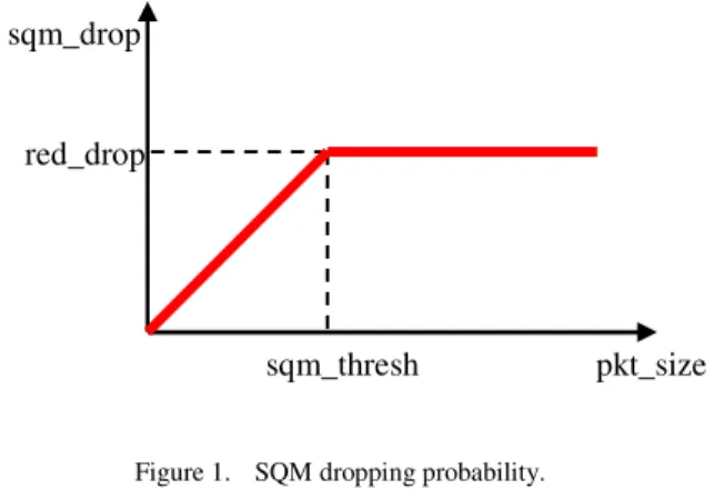
The dropping mechanism is used to classify effectively incoming packets into traffic classes and assign different dropping probabilities. It does so by calculating a threshold, sqm_thresh, which is the moving average of the incoming packets sizes. Every packet bigger than sqm_thresh, will be dropped with the same probability as in a classic RED gateway. However, for smaller packets, the dropping probability will be smaller and proportional to the deviation of the packet size from sqm_thresh. For reasons of clarity, from now on we will refer to packets bigger than sqm_thresh, in a given network topology, as big packets and to packets smaller than sqm_thresh as small packets. The corresponding flows will be named accordingly.
The scheduling mechanism is more sophisticated and works by promoting time-sensitive traffic with delay and low-jitter constraints. When some specific criteria are satisfied, such as when the incoming packet is small or the transport layer protocol of the packet is unresponsive, the router moves a packet
from the end of the queue to the beginning. The queuing delay of the packet is instantly diminished whereas the rest of the packets will experience only trivial delay increase2. Simulation results indicate that packet promotion augments user-perceived quality metrics.
3.1 Dropping policy
SQM keeps track of one variable, sqm_thresh, which is the moving average of all the incoming packet sizes in the router. Since every arrival updates sqm_thresh, its value reflects the current state of the link. Using this dynamic threshold, SQM classifies packets as big and small. If the packet size of the next incoming packet is greater than sqm_thresh, then it will be classified as big, otherwise it will be classified as small. While this classification might seem binary, there are indeed multiple levels of classification for small packets; each packet affects the correlation of packet sizes in the router and is managed differently. Big packets will be dropped with the probability calculated by the original RED algorithm. Small packets, however, will be dropped with smaller probability which will depend on their deviation from sqm_thresh.
If sqm_drop and red_drop are the probabilities of SQM and RED respectively, pkt_size the size of the incoming packet and αa weight factor equal to 0.1, then
• in case pkt_size<sqm_thresh then
thresh sqm size pkt drop red drop sqm _ _ _ _ = (1)
• in case pkt_size≥sqm_thresh then
drop red drop
sqm_ = _ (1)
• finally, sqm_thresh is calculated as follows
(
)
sqm thresh pkt sizethresh
sqm_ = 1−α ⋅ _ +α⋅ _ (3)
Figure 1. SQM dropping probability. 2
We rearrange only when packets are small. Thus, the transmission delay of the packet which equals to the additional queuing delay experience by the rest of the packets will be small.
sqm_drop
red_drop
During the initialization, sqm_thresh is equal to the size of the first arriving packet.
Fig. 1 depicts graphically the Equations (1) and (2).
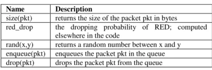
We illustrate the pseudo-code of the SQM dropping algorithm. We consider a router that accepts packets noted as pkt. We use the following variables and functions (Table 1):
TABLE 1. PSEUDO-CODE VARIABLES AND FUNCTIONS
Name Description
size(pkt) returns the size of the packet pkt in bytes red_drop the dropping probability of RED; computed
elsewhere in the code
rand(x,y) returns a random number between x and y enqueue(pkt) enqueues the packet pkt in the queue drop(pkt) drops the packet pkt from the queue
pkt_size=size(pkt) sqm_thresh=0.9*sqm_thresh+0.1* pkt_size if (sqm_thresh<pkt_size) then sqm_drop=red_drop* (pkt_size/sqm_thresh) else sqm_drop=red_drop prop=rand(0,1) if (prop<sqm_drop) then drop(pkt) else enqueue(pkt)
As we see, sqm_thresh depends more on the sizes of recently arrived packets and less on the packets that have recently departed – this renders sqm_thresh an implicit measure of the router’s recent activity. Moreover, by giving equal priority to all packet sizes above sqm_thresh, we manage to serve smaller packets more efficiently but still confine their service with the bandwidth restriction of the fair share. Although the value of the weight factorαmight seem arbitrary, we discuss in section 3.3 its impact on the policy.
That said, a big packet will be dropped always, with a bigger (even only slightly) probability than a small packet. One issue when we design service differentiation policies is to make sure that we are not being unfair to the traffic that we want to demote or punish. That is, we do not want to promote so much a traffic class that the rest of the flows will starve. This issue applies in SQM in cases where we have many small packets and few big packets. In such a case, sqm_thresh will be small and close to the size of small packets. Is it fair to drop the big packets with almost the same probability as the small ones? Shouldn't we drop them with smaller probability, since they have a minor contribution in the contention? In order to be light-weight, SQM uses only one parameter as the threshold for service differentiation; sqm_thresh. This parameter is the combined estimator of the flows number and their packet sizes. The information derived by the router is that, either the majority of packet sizes is close to this estimate, or the packet
sizes are symmetrically distributed around sqm_thresh. Superior knowledge of the router state would require extensive reference tables and time-costly updates. Nevertheless, even if the absolute knowledge of the router state could be available, still we wouldn't like to promote a minority of big packet sizes. The reason is that, by keeping almost the same dropping probability for all packets (in this example), the router would eventually reach the desired equilibrium state. If the small numbers of big packet sizes is produced by an equally small number of flows who cannot generate more traffic, there is no reason of promoting them. If they are produced by a big number of flows who are below their fair share, eventually (due to their responsive transport protocol) they will increase their portion on the congestion, limiting the small packets to their fair share. Besides, according to Fig. 10 where we have a case where small flows gradually increase their number, the current scheme provides an almost ideal ASI as the correlation of packet sizes varies.
3.2 Scheduling policy
In order to provide quality guarantees for time-sensitive flows, we incorporate a scheduling mechanism in SQM. This mechanism promotes some packets to the head of the output queue, immediately upon their arrival. Our scheduling policy relies on only the size of the packets, the overlying transport protocol, as well as, the length of the queue. A packet is promoted if and only if, all four conditions apply:
1. A packet was previously characterized as small, that is pkt_size<sqm_thresh.
2. A packet belongs to an unresponsive flow or the packet is an ACK. We decide that a packet belongs to an unresponsive3flow when it uses UDP4(“Protocol” field for IPv4, or “Next Header” field for IPv6) and that a packet is an ACK, when its size is 40B5. Since we consider UDP, no duplicate acknowledgements are going to be generated due to rearrangement.
3. A packet is not only smaller but much smaller compared to sqm_thresh, or the queue is big and nearly full. This means that we will either promote a very small packet, or a small packet when the queue is almost full and the potential queuing delay very high. Both these conditions are determined probabilistically, i.e. the smaller the packet, the higher the probability to favor it.
4. The router has recently rearranged no more than a fixed, predetermined number of packets (here set to five) in a row. This ensures that packets that fulfill the previous criteria will not monopolize the outgoing
3
This may sound strange. Typically we punish unresponsive flows, instead of promoting them.
4
Although there are several cases where the Application Layer protocol may incorporate reliability, we consider that flows that utilize UDP are generally non-responsive. Nevertheless the algorithm is configurable to add multiple, unresponsive, transport
layer protocols. 5
Routers are by default network layer devices and cannot recognize upper layer headers.
link. We have chosen to rearrange only five packets a time, because after extensive experiments we concluded that this number provided a fair trade-off between performance and service differentiation. While we intend to approximate this variable analytically in the future, for now we will consider it static and equal to five. The rearranged-packet counter is decreased and set to zero when packets that arrive in the queue are not rearranged.
The previous conditions are set as follows:
if ((packet is small) AND
(packet uses UDP or packet is ACK) AND (packet is very small OR queue length is big) AND
(packets already prioritized ? packet_thresh)) then {
prioritize packet
increase prioritized packets counter }
else {
decrease prioritized packets counter ...
}
3.3 The impact of the weight factorα
An important component of SQM that we analyze last is the α variable. We explained earlier why sqm_thresh should reflect the router's current state. As packets of different size populate the queue, sqm_thresh should be able to adjust fast enough to reflect the new state.
0 200 400 600 800 1000 1200 1 4 7 10 13 16 19 22 25 28 31 34 37 40 43 46 49 # of incoming packets s q m _ th re s h α=0.05 α=0.1 α=0.2
Figure 2. Convergence of sqm_thresh with different values ofα. We assume that sqm_thresh=1040B and 140B packets arrive at the router. By setting a=0.1, sqm_thresh's value will be below 150B in 43 steps, or 43 packets. If the buffer's capacity is near 140·43≈6kB then sqm_thresh will reflect only the packets currently in the queue, otherwise a bigger or smaller α value might be more appropriate (this is not exactly accurate however, since sqm_thresh takes account also the sizes of the packets that have been dropped). Different
αvalues result in different convergence times (Fig. 2). For now we consider a static and equal to 0.1.
4. IMPACTANALYSIS
We will now examine the impact of SQM on packet services and specifically on Packet Loss Rate and Queuing Delay. The aim of our analysis is (i) to confirm that SQM promotes performance and quality for small flows and (ii) to investigate whether our policy leads to unfairness or underutilization. The impact of SQM will be examined in contrast with RED, since RED and SQM, as we showed earlier, are based on the same core algorithm.
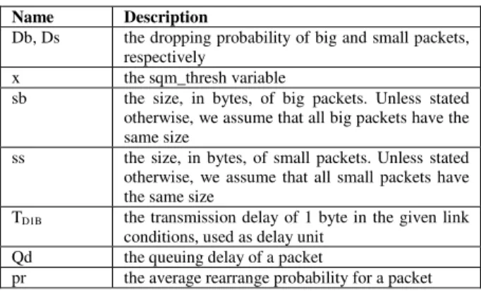
We assume that a small packet may be either rearranged, and consequently forwarded to the outgoing line, or assigned a smaller dropping probability and maybe dropped. During our analysis we use some variables (Table 2). When these variables have the letter R subscripted, they refer to RED, whereas when they have the letter S subscribed, they refer to SQM.
TABLE 2. ANALYSIS VARIABLES
Name Description
Db, Ds the dropping probability of big and small packets, respectively
x the sqm_thresh variable
sb the size, in bytes, of big packets. Unless stated otherwise, we assume that all big packets have the same size
ss the size, in bytes, of small packets. Unless stated otherwise, we assume that all small packets have the same size
TD1B the transmission delay of 1 byte in the given link
conditions, used as delay unit Qd the queuing delay of a packet
pr the average rearrange probability for a packet
4.1 Packet Loss Rate (PLR)
SQM intends to minimize proactive dropping of small packets and maintain, for bigger packets, the dropping rates of RED. We assume that small packets usually characterize real-time data, and in this sense time-sensitive flows. Thus the same effect for small packets is related directly to packet loss and does not impact the transmission rate. However, since SQM does not drop more big packets than RED, its impact on transmission rate is also zero6. To estimate the packet loss rate, we first calculate the dropping probability. Big packets: drop red DbR= _ drop red drop sqm DbS = _ = _ 0 = − =DbS DbR impact (4) 6
In fact, we have increased loss due to the increased queue length which we consider trivial.
Small packets (dropping algorithm): drop red DsR= _ drop red x ss drop sqm DsS = _ = ⋅ _ 0 1 _ < − ⋅ = − = x ss drop red Db Db impact S R (5)
Small packets (scheduling algorithm):
drop red DsR= _ 0 _ = =sqm drop DsS drop red Ds Ds impact= S− R=− _ (6)
Equation (4) demonstrates that SQM does not increase the loss rate of big packets more than RED. Equations (5) and (6), on the other hand, show that SQM decreases or even zeroes the PLR of small packets providing them with the desired privileges. When the dropping algorithm is used alone, loss rate is a function of ss and x. Smaller ss and/or bigger x signify less proactive drops. Since the packet size is determined by the corresponding application and sqm_thresh is determined by the queue, misbehaving becomes more difficult. Intentional data fragmentation may result temporarily in performance benefits. However, as we will show in section 5, there is not a fragmentation policy that can form a solid winning strategy; depending on the transient value of sqm_thresh a user may win (decreased dropping) or lose (increased overhead).
4.2 Queuing delay
We consider a router, where big and small packets (noted as ‘b’ and ‘s’, respectively) have arrived. Some of them have been rearranged while others have not. For those not rearranged, some have been dropped and others have been routed. Small packets that have been rearranged, contribute to the buffer contention, as well. At some random time point in time, a packet arrives. We assume two cases: (i) the packet is small and is rearranged immediately or (ii) the packet is either big or small and not rearranged. In the second case, the impact is the same regardless of the packet size, as it will experience the same queuing delay. This queuing delay will depend on the dropping probabilities of the packets that arrived previously in the queue.
(
)
(
)
(
)
(
bsb s ss red drop b sb s ss)
T drop red T ss s drop red T sb b Qd B D B D B D R ⋅ + ⋅ ⋅ − ⋅ + ⋅ ⋅ = = − ⋅ ⋅ ⋅ + − ⋅ ⋅ ⋅ = _ _ 1 _ 1 1 1 1Small packet promoted by scheduling mechanism:
0 = S Qd ⇔ − =QdS QdR impact
(
1 _) (
)
0 1 ⋅ − ⋅ ⋅ + ⋅ ≤ − = T red drop b sb s ss impact DB (7) Packet routed:(
)
(
)
(
)
(
(
)
(
⋅ + ⋅ ⋅ ⋅ − − + ⋅ ⋅ + ⋅ ⋅ = = − ⋅ + ⋅ ⋅ + + − ⋅ ⋅ ⋅ = = + − ⋅ ⋅ ⋅ + + − ⋅ ⋅ ⋅ = 2 1 1 1 1 1 _ 1 _ 1 _ 1 _ 1 _ 1 ss s x sb b drop red pr ss s sb b T pr drop red x s ss s drop red sb b T pr drop sqm T ss s drop sqm T sb b Qd B D B D B D B D S(
)
(
)
(
⋅ + ⋅ − ⋅ ⋅ + ⋅)
⇔ ⋅ − ⋅ + ⋅ ⋅ ⋅ − + ⋅ ⋅ + ⋅ ⋅ = − = ss s sb b drop red ss s sb b T ss s x sb b drop red pr ss s bs b T Qd Qd impact B D B D R S _ 1 _ 1 1 2 1 0 1 _ 1 ≥ − ⋅ + ⋅ ⋅ ⋅ = x ss drop red pr s ss T impact DB (8) since ss<x.Equation (7) is rather self-explanatory. A rearranged packet will experience zero dropping probability, thus the impact on queuing delay will be maximum. For packets not rearranged, regardless of their size, Equation (8) demonstrates the impact on the queuing delay. Packets will experience increased delay since some small packet that would have otherwise been dropped from the queue, now contribute to delay cumulatively. Big flows, that generally use TCP, will eventually decrease the rate with which they increase their sending windows. Moreover, big packets increase the risk to be dropped due to the increasing competition in the queue that might result in an average queue length that exceeds the maximum threshold. Nevertheless, although small packets might experience bigger delays, most of the times their queuing delay will be zero. Since, however, they are not typically governed by the AIMD (Additive Increase/ Multiplicative Decrease) principle, faster delivery will not trigger transmission rate increase, and hence big flows will not end-up starving for bandwidth. In conclusion, we have proved that SQM can achieve service differentiation by adjusting its services to packet sizes.
5. DEVELOPING INDIVIDUAL STRATEGIES SQM makes the assumption that small packet sizes correspond only to applications that require special service. However, users might try to fragment their bulk data into smaller pieces in order to promote themselves and gain from decreased dropping. We prove in this section using the basic principles of game theory that in SQM, the result of such an action depends on the behavior of the rest of the flows and that it is uncertain whether fragmentation is a winning or losing strategy.
We assume a bulk data application that sends packets of a specific size in a single router network in presence of other flows. After some time, only the aforementioned application changes its attitude and fragments its data into smaller packets.
We will use the variables cited in Table 3. When accentuated, they will refer to variables after fragmentation.
TABLE 3. ANALYSIS VARIABLES
Name Description
x the sqm_thresh variable before fragmentation x' the sqm_thresh variable after fragmentation
ps the total size of the application’s packet before fragmentation
ps' the total size of the application’s packet after fragmentation
pl the payload of the packet od the overhead of the packet
k the fragmentation factor of the packet
ABL an “average bytes lost” index which is the packet size of a packet multiplied by its dropping probability. If
1 ' ABL>
ABL , we lose from fragmentation, otherwise we win
Based on our previous assumptions we examine three main cases which can be concluded in Table 4. This table presents the possible cases from a single-user perspective, before and after fragmentation. For example, case (2) means that the user’s packet size before fragmentation was bigger than sqm_thresh, whereas after fragmentation the new packet size is smaller than the new value of sqm_thresh.
TABLE 4. POSSIBLE OUTCOME FOR A USER,BEFORE AND AFTER FRAGMENTATION Before fragmentation x ps> ps<x ' ' x ps> (1) (4) After fragmentation ps'<x' (2) (3) The fourth case although objects to our assumptions, is possible in practical conditions and thus it will be examined separately.
1) ps>x, ps'>x'
In this first case, even though we fragment, the packet size is still bigger than sqm_thresh.
(
pl od)
red drop drop sqm ps ABL= ⋅ _ = + ⋅ _(
pl k od)
red drop drop red od k pl k drop sqm ps k ABL _ _ _ ' ' ⋅ ⋅ + = = ⋅ + ⋅ = ⋅ ⋅ =(
)
(
)
_ 1 _ ' > + ⋅ + = ⋅ + ⋅ ⋅ + = od pl od k pl drop red od pl drop red od k pl ABL ABL (9)In this case, the more we fragment, the more we lose. 2) ps>x, ps'<x'
(
pl od)
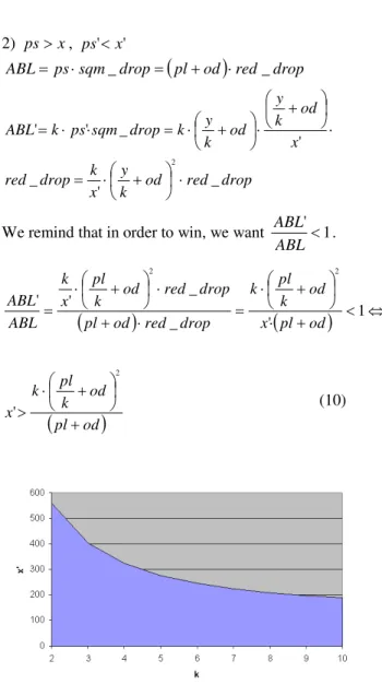
red drop drop sqm ps ABL= ⋅ _ = + ⋅ _ drop red od k y x k drop red x od k y od k y k drop sqm ps k ABL _ ' _ ' _ ' ' 2 ⋅ + ⋅ = ⋅ + ⋅ + ⋅ = ⋅ ⋅ =We remind that in order to win, we want '<1 ABL ABL .
(
)
⋅(
+)
< ⇔ + ⋅ = ⋅ + ⋅ + ⋅ = 1 ' _ _ ' ' 2 2 od pl x od k pl k drop red od pl drop red od k pl x k ABL ABL(
pl od)
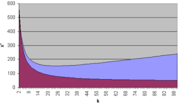
od k pl k x + + ⋅ > 2 ' (10)Figure 3. The x' parameter as a function of the fragmentation factor.
For pl=1000B and od=40B, if x' lies in the blue area in Fig. 3 then we lose, else we win. For relatively small values of k, the above function is constantly decreasing. In this case, we increase our probabilities of winning by increasing k (that is the fragmentation), thus decreasing the packet size. However, for bigger values of k, the function has a negative peak (Fig. 4).
For given pl and od the lower peak is unique. This lower peak defines the point where x' has its lower value. At this point (k=25 in Fig. 4), we have the biggest possibility of winning from fragmentation. However, since we do not know the current value of x', x' may have any value. If x' is either in the blue or the red zone then we lose from fragmentation. The red zone defines the cases where the packet size is bigger than x', thus we fall back to the first case.
Figure 4. The x' parameter and packet size as a function of the fragmentation factor. 3) ps<x, ps'<x'
(
) (
)
(
pl od)
red drop x drop red x od pl od pl drop sqm ps ABL _ 1 _ _ 2⋅ + ⋅ = = ⋅ + ⋅ + = ⋅ = drop red od k pl x k drop red x od k pl od k pl k drop sqm ps k ABL _ ' _ ' _ ' ' 2 ⋅ + ⋅ = ⋅ + ⋅ + ⋅ = ⋅ ⋅ =(
)
(
)
2 2 2 2 ' _ 1 _ ' ' od pl od k pl k x x drop red od pl x drop red od k pl x k ABL ABL + + ⋅ ⋅ = ⋅ + ⋅ ⋅ + ⋅ = (11 )In order to win we must have
(
)
2 2 ' od pl od k pl k x x + + ⋅ >which is a similar function as in the second case. For pl=1000B and od=40B we get the graph in Fig. 5.
Figure 5. The x'/x portion as a function of the fragmentation factor.
Since we assumed that x' is modified only by one flow, we expect that x'/x is near 1. Hence in this case we can be sure that we always win, even though there is a specific packet size that we have the most benefits.
If we cancel the assumption that only one flow alters its stance, or in case that more flows enter the network, then the fourth case is possible.
4) ps<x, ps'>x'
(
) (
)
(
pl od)
red drop x drop red x od pl od pl drop sqm ps ABL _ 1 _ _ 2⋅ + ⋅ = = ⋅ + ⋅ + = ⋅ =(
pl k od)
red drop drop red od k pl k drop sqm ps k ABL _ _ _ ' ' ⋅ ⋅ + = = ⋅ + ⋅ = ⋅ ⋅ =(
)
(
)
(
)
(
+)
< ⇔ ⋅ + ⋅ = ⋅ + ⋅ ⋅ ⋅ + = 1 _ 1 _ ' 2 2 pl od od k pl x drop red od pl x drop red od k pl ABL ABL(
)
(
pl k od)
od pl x ⋅ + + < ⇔ 2 (12)which is impossible, since we supposed that
od pl
x> + . Thus, no matter what we do, we always lose.
We can summarize the previous analysis by saying that if ps'>x' then we certainly lose, otherwise, we may either win or lose. The entire problem resembles the ‘prisoner’s dilema’; if only one user fragments its data he wins, while the other loses, if they both fragment their data, they both lose. We note that the loss is not due to the decreased packet size but because of the increased number of packets the user has to generate to maintain the same sending rate.
6. SIMULATIONS
In order to verify SQM’s ability to enhance quality, we conduct several ns-2 simulations. Our aim is twofold:
i) To prove that network resources are allocated fairly by the system and
ii) To demonstrate that the quality benefits gained by time-sensitive flows have only a minor effect on bulk flows.
We first introduce the evaluating metrics for SQM. We then detail the types of traffic used, as well as the AQM mechanisms with which we compare SQM. We describe the simulation topologies, scenarios and the corresponding results. Finally, we lay our major conclusions from our results.
6.1 Metrics
Goodput: Goodput is used to measure the overall performance of the network in terms of effective bandwidth utilization. onTime Transmissi ta OriginalDa Goodput=
where OriginalData is the number of bytes delivered from a sender to the corresponding receiver during their connection (TransmissionTime), excluding the retransmitted data and the overhead induced by packet headers.
Mean Goodput: Mean Goodput is the average of the Goodput values of the individual flows, where n is the number of flows.
n Goodput t MeanGoodpu n i i
∑
= = 1Packet Loss Rate: Packet Loss Rate (PLR) is the number of lost packets over the total number of transmitted packets. Packets can be lost due to buffer overflows or proactive dropping.
ackets ansmittedP NumberOfTr stPackets NumberOfLo PLR=
Average Packet Loss Rate: Average PLR is the average value of all individual PLRs in the network, where n is the number of flows.
n PLR AvgPLR n i i
∑
= = 1Average Delay: Average Delay is the queuing delay of all the flows of a specific type of traffic, where n is the number of flows.
n Delay AvgDelay n i i
∑
= = 1Application Satisfaction Index: The Application Satisfaction Index (ASI), which was introduced in [25], captures the delay fair share per application on the basis of the delay impact of each application on others. It is defined as:
max 1 max 1 Delay n Delay TotalData Data Delay ASI n i i i ⋅ − − =
∑
=where n is either the number of active nodes or the number of different traffic classes; Datai the total transmitted data of the ith node to the receiver; TotalData the total transmitted data of all nodes; Delayi the average queuing delay of the ith node and Delaymax the maximum queuing delay of the system.
R-Factor: We characterize the quality of voice communication using the R-Factor, which is included in the E-Model ([16], [17]), an ITU-proposed analytic model of voice quality. R-Factor captures voice quality and ranges from 100 to 0, representing best and worst quality respectively. R-Factor incorporates several different parameters, such as echo, background noise, signal loss, codec impairments and others. In [18], R-Factor is defined as:
(
d) (
H d)
(
c)
d a
R= −β1 −β2 −β3 −β3 −γ1−γ2ln1−γ3
where α=94.2, β1=0.024ms-1, β2=0.11ms-1,
β3=177.3ms, expresses the mouth-to-ear delay and the packet loss rate. For the G.711 codec, γ1=0, γ2=30,
γ3=15.
6.2 Types of traffic
We simulate four types of traffic; (i) FTP traffic, which consists of big packet sizes, (ii) FTP traffic, which consists of small packet sizes, (iii) VoIP, which consists of real-time traffic and small packets and (iv) Sensors, which also consist of real-time traffic, however, their packet sizes are smaller than VoIP. The characteristics of each type of traffic are as follows:
Big FTP Traffic: Big FTP packets are carried by the TCP NewReno version. Their size is 1040B.
Small FTP Traffic: Small FTP packets are carried by the TCP NewReno version. Their size is 140B.
VoIP Traffic: VoIP packets are carried by UDP. During a conversation, speakers alternate between activity and idle periods. Taking into consideration the ON and OFF periods [4], as well as the heavy-tailed characteristics and self similarity of VoIP traffic [7], we used the Pareto distribution for modeling the call holding times. We configure Pareto with a mean rate that corresponds to the transmission rate of 64kbps and the shape parameter is set to 1.5. In accordance with [4], we distribute the ON and OFF periods with means of 1.0 sec and 1.35 sec, respectively. We simulate VoIP streams of 64kbps (following the widely-used ITU-T G.711 [6] coding standard) and we set packet sizes at 160 bytes (each packet has 40-byte packet header).
Sensor Traffic: We simulate Sensor flows by sending periodically packets of 40 bytes (20 bytes of sensor data plus a 20-byte packet header) carried by UDP. The interval between two consecutive sensor transmissions is set to 50 ms.
6.3 AQM mechanisms setup
During the experimental evaluation we compare SQM with four other AQM mechanisms: RED, RIO, PI (Proportional Integral scheme) and NCQ+. We use the following sets of RED and NCQ+ parameters:
RED: The RED parameters are set according to the recommendation in [13]. That is, we use the “gentle” mode, the maximum threshold is set to three times the minimum threshold, and the minimum threshold is set to 1/8 of the buffer size. To acquire comparable results, we use RED in byte mode.
RIOand PI: We used the parameters determined by ns-2.
NCQ+: NCQ+ parameters are set according to the recommendations in [22] and [25]. That is ncqthresh1 is set to 0.05 andαis always equal to 0.1.
6.4 Topologies and scenarios
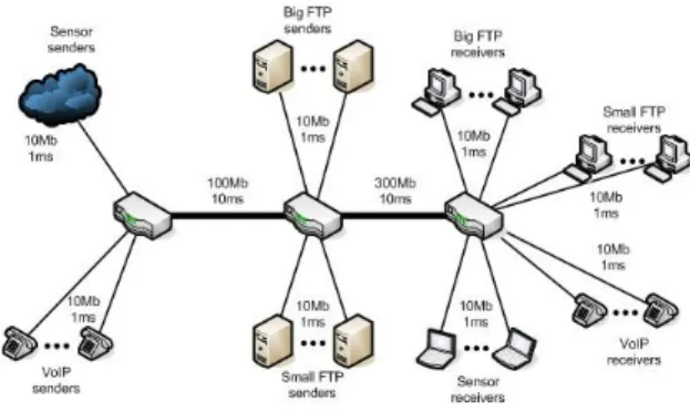
We assume two main topologies; a dumbbell and a cross-traffic. In the dumbbell topology (Fig. 6) we investigate if SQM allocates efficiently network resources or leads some flows to starvation. In the first scenario of this topology we consider a fixed number of 100 big FTP flows and a varying number of VoIP flows from 0 to 200. In the second scenario we invert the participation of the flows in the contention. In the cross-traffic topology (Fig. 7) we examine SQM scalability. The percentages of each type of traffic are fixed and equal to 40% for big FTP flows, 40% for small FTP flows, 10% for VoIP flows and 10% for sensor flows. During the first phase of our evaluation we set the total number of flows to 500 and we gradually increased it until the total number of flows reached 1000; our intention was to prove SQM ability to administer different types of traffic, as well as to verify its adaptability to different levels of contention. Due to lack of space we present only the last set of simulations where the total number of flows equals to 1000. The rest of the simulations manifested similar behavior. Their results are presented in [10].
Figure 6. Dumbbell topology.
Figure 7. Cross-traffic topology.
6.4.1 Varying number of VoIP flows
In the first scenario, we consider 100 big FTP flows and we gradually increase the number of VoIP flows from 0 to 200. We measure the number of successfully received packets for each type of flow, as well as the R-Factor and ASI indexes.
The results are shown in Fig. 8-11 and demonstrate SQM ability to provide quality guarantees for time-sensitive flows. In Fig. 8 and 9 we can see that SQM achieves better buffer utilization than the rest of the schemes. VoIP sent packets are increased at least 30% (from 35,000 to 45,000 packets for 200 VoIP flow), with only a 2% decrease for big FTP packets. This prioritization, which results also in smaller queuing delays for VoIP packets, allows SQM to score highly both on ASI (60% increase) and on Factor (25% increase). We should note that the R-Factor achieved by SQM is the biggest possible value for the coding we used (G.711).
Big FTP received packets
53000 54000 55000 56000 57000 58000 59000 60000 0 25 50 75 100 125 150 175 200 VoIP flows re c e iv e d p a c k e ts RED RIO PI NCQ+ SQM
Figure 8. Big FTP received packets.
VoIP received packets
0 5000 10000 15000 20000 25000 30000 35000 40000 45000 50000 0 25 50 75 100 125 150 175 200 VoIP flows re c e iv e d p a c k e ts RED RIO PI NCQ+ SQM
ASI 0,5 0,55 0,6 0,65 0,7 0,75 0,8 0,85 0 25 50 75 100 125 150 175 200 VoIP flows A S I RED RIO PI NCQ+ SQM Figure 10. ASI. R-Factor 0 10 20 30 40 50 60 70 80 90 100 0 25 50 75 100 125 150 175 200 VoIP flows R -F a c to r REDRIO PI NCQ+ SQM Figure 11. R-factor.
6.4.2 Varying number of big FTP flows
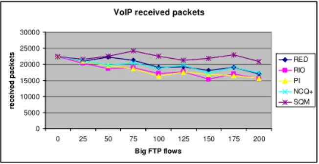
In the second scenario we invert the application analogy; we now consider 100 VoIP flows and we gradually increase the number of big FTP flows from 0 to 200. Our aim this time is to show that although the proportion of bulk data may increase in a network, SQM always allocates buffer space for real-time flows but not at the expense of big flows.
Big FTP received packets
53000 54000 55000 56000 57000 58000 59000 60000 0 25 50 75 100 125 150 175 200 Big FTP flows re c e iv e d p a c k e ts RED RIO PI NCQ+ SQM
Figure 12. Big FTP received packets.
VoIP received packets
0 5000 10000 15000 20000 25000 30000 0 25 50 75 100 125 150 175 200 Big FTP flows re c e iv e d p a c k e ts RED RIO PI NCQ+ SQM
Figure 13. VoIP received packets.
ASI 0,5 0,6 0,7 0,8 0,9 1 0 25 50 75 100 125 150 175 200 Big FTP flows A S I RED RIO PI NCQ+ SQM Figure 14. ASI. R-Factor 40 50 60 70 80 90 100 0 25 50 75 100 125 150 175 200 Big FTP flows R -F a c to r REDRIO PI NCQ+ SQM Figure 15. R-factor.
The results are depicted in Fig. 12-15. Even when bigger flows dominate the network, SQM adaptive prioritization allows small flows to maintain almost stable transmission rate. As more big packets arrive in the queue, sqm_thresh is being increased, leading in smaller dropping probability for small packets and hence enhancing their service. The stability in Fig. 14 and 15 is due to the scheduling mechanism that minimizes the queuing delay of VoIP packets. Once again big packets experience only a 2% less packet reception which, as Fig. 14 demonstrates, probably the users will not notice at all.
6.4.3 Cross-traffic scenario
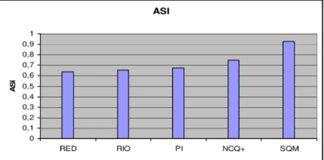
In this scenario we consider the cross-traffic topology of Fig. 7, where the proportions of different types of traffic are fixed (40% big FTP flows, 40% small FTP flows, 10% VoIP flows and 10% sensor flows) and the total number of flows is 1000. The results for smaller number of flows are similar. In Fig. 16 we demonstrate the PLR inflicted by proactive
dropping. SQM is the only scheme that achieves such a good classification of bulk and real-time data. The dropping mechanism does not discriminate between responsive and unresponsive, and thus small FTP packets are prioritized as well. This prioritization results in increased Goodput, as can be seen in Fig. 17. Nevertheless, the average Goodput of small FTP flows is still smaller than the average Goodput of big FTP flows. Average PLR 0 0,02 0,04 0,06 0,08 0,1 0,12 0,14 0,16 0,18
Big FTP Small FTP VoIP Sensor
ra te RED RIO PI NCQ+ SQM Figure 16. Average PLR. Average Goodput 0 0,01 0,02 0,03 0,04 0,05 0,06 0,07 0,08 0,09
Big FTP Small FTP VoIP Sensor
M b p s RED RIO PI NCQ+ SQM
Figure 17. Average Goodput.
Average Delay 0 1 2 3 4 5 6 7 8 9 10
Big FTP Small FTP VoIP Sensor
m s e c RED RIO PI NCQ+ SQM
Figure 18. Average delay.
ASI 0 0,1 0,2 0,3 0,4 0,5 0,6 0,7 0,8 0,9 1 RED RIO PI NCQ+ SQM A S I Figure 19. ASI.
Fig. 14 depicts the average queuing delay experienced by the various types of traffic. VoIP and sensor traffic experiences significantly less queuing delay, while FTP flows experience more.
7. CONCLUSIONS AND FUTURE WORK
Did SQM succeed to satisfy more users? Fig. 15 demonstrates that it did. SQM results in 25%-50% increase in ASI, leading to better bandwidth redistribution. We also demonstrated how SQM classifies traffic and how it applies different policies to each packet depending its size, the sizes of packets currently in the queue and the contention levels in the router. Simulation results indicated that SQM is indeed practical and efficient. Our future plans include integrating SQM in a routing device, in order to obtain results that will assist us to calibrate our scheme into a more realistic behavior.
REFERENCES
[1] S. Blake, D. Black, M. Carlson, E. Davies, Z. Wang, and W. Weiss, “RFC2475 - An Architecture for Differentiated Services”, December 1998.
[2] U. Bodin, O. Schelen, and S. Pink, “Load-tolerant Differentiation with Active Queue Management”, ACM SIGCOMM Computer Communication Review, vol. 30, iss. 3, pp. 4 – 16, July 2000.
[3] R. Braden, D. Clark, and S. Shenker, “RFC2475 - Integrated Services in the Internet Architecture: an Overview”, June 1994.
[4] P. Brady, “A Statistical Analysis of On-Off Patterns in 16 Conversations”, The Bell System Technical Journal, vol. 47, pp. 73 – 91, 1968.
[5] D. Clark, and W. Fang, “Explicit allocation of best-effort packet delivery service”, IEEE/ACM Transactions on Networking, vol. 6, iss. 4, pp. 362 – 373, August 1998. [6] R. Cole and J. Rosenluth, “Voice over IP Performance
Monitoring”, ACM SIGCOMM Computer Communications Review, vol. 31, iss. 2, pp. 9 – 24, April 2001.
[7] T. Dang, B. Sonkoly, and S. Molnar, “Fractal Analysis and Modelling of VoIP Traffic”, Networks 2004, June 2004. [8] S. Dimitriou and V. Tsaoussidis, “Adaptive Head-to-Tail:
Active Queue Management based on implicit congestion signals”, Elsevier Computer Communications, vol. 32, iss. 2, pp. 246 – 256, February 2009.
[9] S. Dimitriou and V. Tsaoussidis, “A New Service Differentiation Scheme: Size Based Treatment”, ICT 2008, June 2008.
[10] S. Dimitriou and V. Tsaoussids, “Evaluation of LIBS-oriented strategies for Service Differentiation”, TR-DUTH-EE-2009-2.
[11] S. Dimitriou and V. Tsaoussidis, “Introducing Size-oriented Dropping Policies as QoS-supportive functions”, IEEE Transactions on Network and Service Management, vol. 7, iss. 1, pp. 13 – 27, March 2010.
[12] C. Dovrolis, D. Stiliadis, and P. Ramathan, “Proportional differentiated services: delay differentiation and packet scheduling”, IEEE/ACM Transactions on Networking, vol. 10, iss. 1, pp. 12 – 26, February 2002.
[13] S. Floyd, “RED: Discussions of Setting Parameters”, November 1997.
[14] S. Floyd and K. Fall, “Promoting the use of end-to-end congestion control in the Internet”, IEEE/ACM Transactions on Networking, vol. 7, iss. 4, pp. 458 – 472, August 1999. [15] C.V. Hollot, Vishal Misra, Don Towsley, and W. Gong, “On
Designing Improved Controllers for AQM Routers Supporting TCP Flows”, IEEE Infocom 2001, April 2001.
[16] ITU-T Recommendation G.107, “The E-Model, a Computational Model for Use in Transmission Planning”, December 1998.
[17] ITU-T Recommendation G.113, “General Characteristics of General Telephone Connections and Telephone Circuits -Transmission Impairments”, February 1996.
[18] ITU-T Recommendation G.711, “Pulse Code Modulation (PCM) of Voice Frequencies”, November 1988.
[19] L. Le, K. Jeffay, and F. D. Smith, “A Loss and Queuing-Delay Controller for Router Buffer Management”, ICDCS 2006, July 2006.
[20] D. Lin, and R. Morris, “Dynamics of Random Early Detection”, SIGCOMM 1997, September 1997.
[21] R. Mahajan, and S. Floyd, “Controlling High Bandwidth Flows at the Congested Router”, ICNP 2001, November 2001. [22] L. Mamatas, and V. Tsaoussidis, “A new approach to Service Differentiation: Non-Congestive Queueing”, CONWIN 2005, July 2005.
[23] L. Mamatas and V. Tsaoussidis, “Differentiating Services with Non-Congestive Queuing (NCQ)”, IEEE Transactions on Computers, vol. 58, iss. 5, pp. 591 – 604, May 2009. [24] R. Pan, B. Prabhakar, and K. Psounis, “CHOKe: a stateless
AQM scheme for approximating fair bandwidth allocation”, INFOCOM 2000, March 2000.
[25] G. Papastergiou, C. Georgiou, L. Mamatas and V. Tsaoussidis, “On Short Packets First: A delay-oriented prioritization policy”, Technical Report TR: DUTH-EE-2008-8.
[26] I. Stoica, S. Shenker, and H. Zhang, “Core-Stateless Fair Queueing: A Scalable Architecture to Approximate Fair Bandwidth Allocations in High Speed Networks”, IEEE/ACM Transactions on Networking, vol. 11, iss. 1, pp. 33 – 46, February 2003.
[27] J. Wei, C.-Z. Xu, X. Zhou and Q. Li, “A robust packet scheduling algorithm for proportional delay differentiation services”, GLOBECOM 2004, November 2004.