Quantum Control of Open Systems and Dense Atomic Ensembles

(1)

University of Windsor University of Windsor

Scholarship at UWindsor

Electronic Theses and Dissertations Theses, Dissertations, and Major Papers

2017

Quantum Control of Open Systems and Dense Atomic Ensembles

Christopher DiLoreto

University of Windsor

Follow this and additional works at: https://scholar.uwindsor.ca/etd

Recommended Citation Recommended Citation

DiLoreto, Christopher, "Quantum Control of Open Systems and Dense Atomic Ensembles" (2017). Electronic Theses and Dissertations. 5976.

https://scholar.uwindsor.ca/etd/5976

This online database contains the full-text of PhD dissertations and Masters’ theses of University of Windsor students from 1954 forward. These documents are made available for personal study and research purposes only, in accordance with the Canadian Copyright Act and the Creative Commons license—CC BY-NC-ND (Attribution, Non-Commercial, No Derivative Works). Under this license, works must always be attributed to the copyright holder (original author), cannot be used for any commercial purposes, and may not be altered. Any other use would require the permission of the copyright holder. Students may inquire about withdrawing their dissertation and/or thesis from this database. For additional inquiries, please contact the repository administrator via email

(2)

Quantum Control of Open Systems and Dense Atomic

Ensembles

By

Christopher DiLoreto

A Dissertation

Submitted to the Faculty of Graduate Studies through the Department of Physics in Partial Fulfillment of the Requirements for

the Degree of Doctor of Philosophy at the University of Windsor

Windsor, Ontario, Canada

2017

(3)

Quantum Control of Open Systems and Dense Atomic

Ensembles

by

Christopher DiLoreto APPROVED BY:

M. Spanner, External Examiner University of Ottawa

J. Gauld

Department of Chemistry

E.H. Kim

Department of Physics

G.W.F. Drake Department of Physics

C. Rangan, Advisor Department of Physics

(4)

Declaration of Previous Publication

This thesis includes an original paper that has been previously published/submitted for publication in peer reviewed journals, as follows:

Thesis Chapter Publication title/full citation Publication status

Chapter 3 C.S. DiLoreto and C. Rangan. Polarization control of spontaneous emission for rapid quantum-state initialization. Phys. Rev. A, 95:043834, 2017.

Published

I certify that I have obtained a written permission from the copyright owner(s) to include the above published material(s) in my thesis. I certify that the above ma-terial describes work completed during my registration as a graduate student at the University of Windsor.

(5)

Abstract

Controlling the dynamics of open quantum systems; i.e. quantum systems that decohere because of interactions with the environment, is an active area of research with many applications in quantum optics and quantum computation. My thesis expands the scope of this inquiry by seeking to control open systems in proximity to an additional system. The latter could be a classical system such as metal nanoparticles, or a quantum system such as a cluster of similar atoms. By modelling the interactions between the systems, we are able to expand the accessible state space of the quantum system in question.

For a single, three-level quantum system, I examine isolated systems that have only normal spontaneous emission. I then show that intensity-intensity correlation spectra, which depend directly on the density matrix of the system, can be used detect whether transitions share a common energy level. This detection is possible due to the presence of quantum interference effects between two transitions if they are connected. This effect allows one to asses energy level structure diagrams in complex atoms/molecules.

By placing an open quantum system near a nanoparticle dimer, I show that the spontaneous emission rate of the system can be changed “on demand” by changing the polarization of an incident, driving field. In a three-level, Λ system, this allows a qubit to both retain high qubit fidelity when it is operating, and to be rapidly initialized to a pure state once it is rendered unusable by decoherence. This type of behaviour is not possible in a single open quantum system; therefore adding a classical system nearby extends the overall control space of the quantum system.

(6)

dense ensemble of atoms rapidly becomes disordered with states that are not directly excited by an incident field becoming significantly populated. This effect motivates the need for using multi-directional basis sets in theoretical analysis of dense quantum systems. My results demonstrate the shortcomings of short-pulse techniques used in many recent studies.

(7)

Acknowledgements

(8)

List of Figures

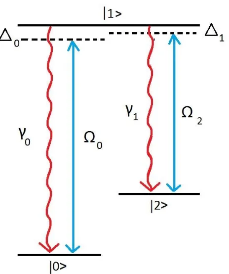
2.1 Schematic of the model three-level Λ system. The two transitions of the Λ are driven by the fields with Rabi frequencies Ω0 and Ω2respectively..

The detuning of the incident field from each of the transitions (∆0 and

∆1) are not equal in general. . . 12

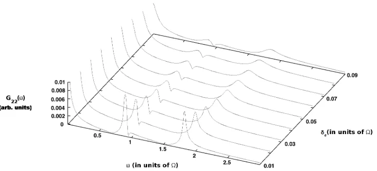
2.2 Intensity-intensity correlation spectra for varying values of detuning

41 with Ω0 = Ω2 = Ω. The detuning 40 is kept fixed at a value of

1.0 Ω. The spontaneous decay rate from the excited state is low with γ/Ω = 0.01. . . 17 2.3 Intensity-intensity correlation spectra of a fluorescent transition in a

Λ system for various values of 41 for 40 = 0. Both transitions are

driven by the same Rabi frequency Ω. The rate of spontaneous decay is low with γ <<Ω. . . 18 2.4 Intensity-intensity correlation spectra for increasing amounts of

spon-taneous decay γ with fixed detuning 41 = Ω₂, and 40 = 0. As the

rate of spontaneous decay increases, the peaks broaden and become less distinguishable. . . 20 2.5 Intensity-intensity correlation spectra for increasing amounts of

de-phasingδd=δ0 =δ2 with fixed detuning 41 = Ω₂, and 40 = 0 as well

(13)

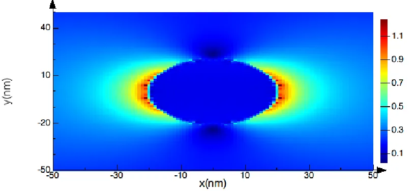
3.1 An xy plot of electric field intensities (|E|at 475 nm) for a ˆypolarizaed wave travelling in the ˆz direction around a 20 nm Ag nanoparticle. . . 30 3.2 A plot of electric field intensity enhancement (|E|/E0) as a function

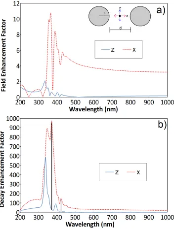
of wavelength for a ˆy polarized wave travelling in the ˆz direction at distance of 10 nm from the surface of a spherical Ag nanoparticle or radiusr. . . 31 3.3 (a) Field enhancements (ME,i=|Ei|/E0) and (b) decay rate

modifica-tion (Md = γ/γ0) of the quantum emitter placed halfway in between

two silver NPs with r = 20 nm and d = 12nm surface-to-surface sep-aration for two different incident polarizations. The blue, solid (red, dashed) curves corresponds to when the incident field is perpendicular (parallel) to the interparticle axis. The two solid vertical lines in (b) correspond to the maximum decay rate enhancement for the ˆx orienta-tion ( 370 nm) and the largest relative ratio of decay rate enhancement, ˆ

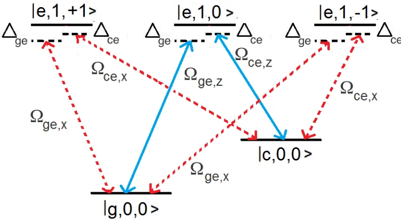
x/zˆ(≈420 nm). . . 36 3.4 Polarization control scheme for rapid qubit initialization. Two applied

fields near resonant with the|gi-|eiand|ci-|eitransitions are linearly polarized in the x−z plane. The z components of the field excite the blue (solid) transitions, while the xcomponents of the field excite the red (dashed) transitions. For preparation, the Rabi frequencies of all transitions are high with respect to spontaneous decay rates. The spontaneous emission rates of the operational (blue, solid) transitions, γge,z and γce,z, stay low, whereas those of the preparation transitions

(red, dashed),γge,x, and γce,x, are greatly enhanced. The detunings are

(14)

3.5 The time required to reach a final, pure state is plotted with respect to the ratio of spontaneous decay rates (γge,x/γge,z = γce,x/γce,z) for

various driving field strengths. The effective five level system is initially driven from an operational, completely mixed state (ρgg =ρ(e,0)(e,0) = ρcc = 1₃). The calculation parameters are Ωce,x= Ωge,x = Ωce,z = Ωge,z,

γge,x = γce,x = γe,x and γge,z = γce,z = γe,z . The preparation time is

normalized to the time taken for an equivalent three-level λ system to reach a steady state. . . 41

4.1 a) When the polarization of an electromagnetic field sets the quan-tization axis of an atom, the effective quantum system is a two-level system with the direction of the transition dipole oriented along that polarization direction. b) When the polarization of an incident control field is different from the quantization axis, the effective quantum sys-tem is a four-level syssys-tem with a dipole transition oriented along each field component. . . 48 4.2 Electric field spectra for different time windows outside a 10 nm radius

nanosphere of atoms with on-resonant excitation located at a spatial position y=3 nm outside the nansophere. Surface plasmons are created by illumation with a monochromatic field of f=2.41×1014 _{Hz and E}

(15)

4.3 Snapshots of ˆy and ˆx direction free currents (in A/m2_{) showing the}

ordered and disordered phases in both the incident field polarization direction (a, b, c - ˆy) and a non-principle direction (d, e, f - ˆx) in a 10 nm nanosphere of atoms at times (a/d) 10 fs, (b/e) 100 fs and (c/f) 250 fs. Populations are evaluated using a 1 nm grid and are illuminated with a constant field intensity of E=1.5×109 V/m. The system has degenerate energy level spacings in the x, y and z direction of 1 eV and a number density of 4×1027 atoms per cubic metre. The beam is polarized in the ˆz direction and the snapshot bisects the nanosphere in the xy plane. . . 55 4.4 Schematic of different regimes in the evolution of a dense quantum

ensemble excited principally along the ˆy direction. (a) In the short time regimes, the ensemble behaves in a similar fashion to a single quantum element - all individual components are in phase and dis-play a uniform oscillation. (b) Entropy is introduced to the system, transitioning it from a uniform ordered phase to a disordered phase with multi-directional excited states. (c) This system is in a disor-dered phase and has all directional states excited to some degree. In this phase it operates in a similar fashion to a classical discrete dipole system as the coherent oscillations are suppressed by directional state leakage. . . 56 4.5 Spatially averaged excited state populations in the ˆx, ˆyand ˆzdirections

for a 10 nm radius nanosphere of atoms with various number densities. Populations are evaluated using a 1 nm grid and are illuminated with a constant field intensity of E=1.5×109_{V/m. The system has degenerate}

(16)

4.5 Spatially averaged excited state populations in the ˆx, ˆyand ˆzdirections for a 10 nm radius nanosphere of atoms with various number densities. Populations are evaluated using a 1 nm grid and are illuminated with a constant field intensity of E=1.5×109_{V/m. The system has degenerate}

energy level spacings in the x, y and z direction of 1 eV. . . 59 4.5 Spatially averaged excited state populations in the ˆx, ˆyand ˆzdirections

for a 10 nm radius nanosphere of atoms with various number densities. Populations are evaluated using a 1 nm grid and are illuminated with a constant field intensity of E=1.5×109_{V/m. The system has degenerate}

energy level spacings in the x, y and z direction of 1 eV. . . 60 4.6 Spatially averaged excited state populations in the ˆx, ˆyand ˆzdirections

for a 10 nm radius nanosphere of atoms with lower energy off-resonant excitation. Populations are evaluated using a 1 nm grid and are illumi-nated with a constant field intensity of E=1.5×109 V/m. The system has degenerate energy level spacings in the x, y and z direction of 1 eV and a number density of 5×1027 _{atoms per cubic metre.} _{. . . .} ₆₁

4.6 Spatially averaged excited state populations in the ˆx, ˆyand ˆzdirections for a 10 nm radius nanosphere of atoms with lower energy off-resonant excitation. Populations are evaluated using a 1 nm grid and are illumi-nated with a constant field intensity of E=1.5×109 _{V/m. The system}

(17)

4.6 Spatially averaged excited state populations in the ˆx, ˆyand ˆzdirections for a 10 nm radius nanosphere of atoms with lower energy off-resonant excitation. Populations are evaluated using a 1 nm grid and are illumi-nated with a constant field intensity of E=1.5×109 _{V/m. The system}

has degenerate energy level spacings in the x, y and z direction of 1 eV and a number density of 5×1027 atoms per cubic metre. . . 63 4.7 Spatially averaged excited state populations in the ˆx, ˆyand ˆzdirections

for a 10 nm radius nanosphere of atoms with higher energy off-resonant excitation. Populations are evaluated using a 1 nm grid and are illumi-nated with a constant field intensity of E=1.5×109 _{V/m. The system}

has degenerate energy level spacings in the x, y and z direction of 1 eV and a number density of 5×1027 _{atoms per cubic metre.} _{. . . .} ₆₄

4.7 Spatially averaged excited state populations in the ˆx, ˆyand ˆzdirections for a 10 nm radius nanosphere of atoms with higher energy off-resonant excitation. Populations are evaluated using a 1 nm grid and are illumi-nated with a constant field intensity of E=1.5×109 _{V/m. The system}

has degenerate energy level spacings in the x, y and z direction of 1 eV and a number density of 5×1027 _{atoms per cubic metre.} _{. . . .} ₆₅

(18)

4.8 Effective ensemble decay rates (γens) for a 10 nm radius nanosphere of

atoms with varying number density (Na). Populations are evaluated

using a 1 nm grid and are illuminated with a constant field intensity of E=1.5×109 _{V/m. The system has degenerate energy level spacings in}

the x, y and z direction of 1 eV. The base decay rate for the individual quantum systems is 2.6×106s−1 . . . 70 4.9 Effective ensemble decay rates (γens) for a 10 nm radius nanosphere of

atoms with varying number density (Na). Populations are evaluated

using a 1 nm grid and are illuminated with a constant field intensity of E=7.5×108 _{V/m. The system has degenerate energy level spacings in}

the x, y and z direction of 1 eV. The base decay rate for the individual quantum systems is 2.6×106_s−1 _{and a logistic function is fit to the}

data. . . 72

5.1 When significant dipole-dipole interactions are present in an ensemble system, it becomes possible for spontaneous emission from one excited state to excite state population from the ground state to another ex-cited state. This allows for “spontaneous-emission” to occur between optically forbidden transitions using emission followed by absorption (δ’s in green). This results in a modified Lindblad decay scheme when examining ensemble populations. δxx, δyy and δzz reflect “parallel”

transitions, whereas δxy, δyz, and δzx reflect “perpendicular”

(19)

5.2 Spatially averaged excited state populations for a 10 nm radius nanosphere of atoms. Populations are evaluated using a 1 nm grid and are illumi-nated with a constant field intensity of E=1.5×109 _{V/m. The system}

has degenerate energy level spacings in the x, y and z direction of 1 eV and a number density of 4×1027 _{atoms per cubic metre. A single}

particle calculation in the RWA approximation is overlaid to compare the two models. . . 81 5.3 Spatially averaged excited state populations for a 10 nm radius nanosphere

of atoms. Populations are evaluated using a 1 nm grid and are illu-minated with a constant field intensity of E = 1.5×109 _{V/m. The}

system has degenerate energy level spacings in the x, y and z direction of 1 eV and a number density of 2.5×1027 _{atoms per cubic metre.}

A single particle calculation in the RWA approximation is overlaid to compare the two models. . . 82 5.4 Full Ensemble Calculation: Spatially averaged excited state

popula-tions for a 10 nm radius nanosphere of an atoms with various number densities. Populations are evaluated using a 1 nm grid and are illumi-nated with a 20 fs width Gaussian pulse. The system has degenerate energy level spacings of 1 eV and a number density of 1×1027 _atoms

per cubic metre. . . 85 5.5 Excited state populations for a Lindblad dissipation evolution scheme

(20)

5.6 Excited state populations for a Lindblad dissipation evolution scheme with decay coupling parameters found by examining state evolution in Fig 5.4. The system evolves from an almost pure excited state and spontaneous emission from this state is able to excite other transitions. For this case, coupling parameters follow the dependence on the density matrix outlined in Section 5.1. . . 89

A.1 Pictorial representation of the process of determining the unitary trans-formation matrix in a 5 level chain. (A) Each transition connects two levels and all edges oscillate at some fast frequency (this oscillation is represented by a circle). A reference level (|3i) is chosen and Uref

is applied. (b) With |3i serving as a reference level (indicated by di-agonal lines under the energy level), the nearest left (|3i → |2i) and right (|3i → |4i) transitions are selected for minimization using rota-tion R0. (c) The previous rotation, R0 which affects all nodes to the left (blue arrow) and to the right (green arrow) removes the oscillation in|3i → |2i and |3i → |4i. The next nearest left (|2i → |1i) and right (|4i → |5i) transitions are then selected for minimization using rota-tion R1_{. (d) Applying}_R1 _{(orange/red arrows) minimizes all rotations}

and the process is complete. . . 102

C.1 Ground state populations and coherences of the qubit with γ = 2.81×

1010s−1 and 4 = 1.37× 1014s−1 is evolved from a variety of initial conditions to reach the desired state populations ρgg= 0.75 andρee =

0.25 . . . 112 C.2 Purity of the qubit, with γ = 2.81×1010_s−1 _and ₄ _{= 1}_.₃₇_×₁₀14_s−1_,

(21)

C.3 The time required to reach a steady state in a three-level lambda sys-tem, normalized to the case in which one decay rate is negligable when compared to the other, is plotted versus various ratios of decay rates. 117

(22)

Glossary of Symbols

Parameter Symbol Description Formula/Value

Energy Level En Energy level of a given state N/A

Transition Fre-quency

ωnm Frequency corresponding to

the energy level separation between levels n and m

En−Em

~

Field Frequency ωk Frequency corresponding to

an incident field frequency

N/A

Incident Electric Field Amplitude

E Amplitude corresponding to an incident electric field

N/A

Local Electric Field

E(r, t) Positional electric field N/A

Local Magnetic Field

B(r, t) Positional magnetic field N/A

Dipole moment µmn Dipole moment of a specific

amount transition dipole between levels n and m

≈(0.1 nm) e

Rabi Frequency Ωnm Rabi frequency

correspond-ing to the transition be-tween level n and m

Ωnm = µmn·E(t) ~

Spontaneous Decay Rate

γnm Rate corresponding to the

decay of|ni → |mi

(23)

Parameter Symbol Decription Formula/Value

Dephasing Rate δmm Rate corresponding to the

dephasing in the transition with upper level |mi

N/A

Detuning 4k Frequency corresponding to

the difference between an incident field frequency and the transition frequency

4k =ωnm−ωk

Number Density Na Number of atoms per unit

volume

(24)

Chapter 1 Introduction

Controlling the dynamics of quantum systems (quantum control [1, 2, 3]) is essential for various applications such as coherently populating specific atomic or molecular eigenstates [4], causing atomic gases to become selectively transparent to specific wavelengths of light [5] and performing computational logic operations on groups of atoms [6, 7]. In all of these applications, the quantum system has a negligible or constant interaction with its environment. The overall effects of these external in-teractions can be modelled by one or more constant decoherence rates (γ) [8]. In theoretical calculations, the assumption that the environmental interaction is negli-gible or constant greatly simplifies the complexity of a system and how to control its behaviour. In this work, I explore the effects of time-dependent decoherence rates, with these we can extend the overall quantum control space, and find novel ways to exploit decoherence-dependent processes.

(25)

system and that of the environment change over time [10, 11, 12]. This is particularly important when the interaction with the environment is dependent. The time-dependent environmental interaction increases the overall number of possible process “knobs” that we can use for quantum control.

Coherent control of quantum systems is typically applied through the use of pre-cise, pulsed-laser excitations which can drive specific transitions, and change the state of the system from one superposition of eigenstates to another [13, 14]. By properly timing and shaping these laser excitations, the system can ideally be driven to almost any state desired [15, 16].

There are, however, many factors that can affect how atoms respond to external stimuli, which complicates this external form of control. This is true in both aggre-gate and individual systems; these systems can have multiple quantum transitions connected by shared levels, and these transitions do not respond independently of one another [17, 18, 19]. In these types of systems, purely quantum effects arise due to the interference between different transitions. This requires us to apply control techniques to a system as a whole, as opposed to viewing the system as a series of independent transitions [20].

1.1 Dissertation Overview

(26)

• Firstly, I look at the control of a single open quantum system with negligible or constant environmental interactions.

• Secondly, I look an open quantum system that interacts with a nearby classical system. The quantum system’s environment is spatially non-uniform; however, the environment does not have an explicit time-dependence.

• Thirdly, I examine a quantum system interacting with a number of identical quantum systems. The environment of a single one in the ensemble is fully quantum mechanical in nature. In this case, the decoherence rates of a single system could be time-dependent.

• Lastly, I propose a model for evaluating the behaviour of a dense ensemble of quantum systems using single-particle techniques. This model is significantly faster to implement computationally than the multi-particle model, and pro-vides a greater understanding of the underlying physics involved. I then use this model to provide a simple explanation for an unusual experimental effect.

1.1.1 Control of a Single, Open Quantum System

In Chapter 2, I investigate an open quantum system exposed to an incident elec-tromagnetic field. In these systems, quantum interference effects occur between con-nected transitions and complicated the evolution of the system’s state. These interfer-ence effects have been both theoretically predicted and measured [22, 23, 24, 25, 26]; however, they have largely been used with the “two-photon resonance” condition to show effects such as correlated and anti-correlated spectra in pairs of transitions.

(27)

intensity-intensity correlation function [27] as a function of the detuning of a single quantum transition, one can detect the presence of connected transitions. This serves as a simple, direct way of confirming energy level diagrams in complex systems. In addition, this method could also be used to track real-time changes in state energy-levels due to ambient interactions.

1.1.2 Control of an Open Quantum System Interacting with

a Nearby Classical System

In Chapter 3, I investigate how the asymmetric enhancement of the decoherence rate of a quantum system can be used to increase the usable “uptime” of quantum information systems by reducing the required “cooling” time in which the system is allowed to spontaneously decay back down to the ground state. This rapid state initialization is another of the main requirements for the practical implementation of quantum computers [28]; however it is largely neglected due to the greater difficulty in obtaining qubits with long lifetimes. As such, my improvement scheme presents a significant advance over typical qubit enhancement schemes [29, 30, 31, 32, 33] which all attempt to reduce the overall decoherence of the system.

(28)

pa-rameter. Using this effect, I have proposed a novel way of changing the spontaneous emission of a system “on demand”. The field-polarization can also affect the purity of the quantum system, which is a useful metric that serves as an indicator of qubit quality [30].

For this investigation, I have left the choice of quantum system general to allow for experimental freedom. These solid state quantum systems could take the form of semiconducting quantum dots [37, 38, 39], or Josephson junctions [40, 41]. Although we have used a nanoparticle, the nearby classical system could be also be a cavity [42, 43, 44, 45] or photonic crystal [46] as along as the system is capable of asymmetrically enhancing a quantum system’s spontaneous emission rate.

1.1.3 Evolution of Dense Quantum Ensembles

In Chapter 4, I examine the control of systems in which the behaviour of a quantum system depends on its environment, which can also be a quantum system. Developing techniques for evaluating the quantum response of nanoscale systems has become an important, recent area of investigation as quantum-based optical effects allow for the design of systems with unique properties [47, 48, 49].

(29)

of decoherence.

As such, I investigated the quantum optical response of nanoscale quantum sys-tems to more intense incident fields, longer timescales and with a multi-directional state basis. The study of this type of system requires the implementation of a new methodology in which quantum evolution and electromagnetic field propagation are solved concurrently. This type of investigation allows for the direct testing of com-putational assumptions that are typically used in the literature.

This work was also motivated by the potential application of dense quantum systems to enhancing the response of solar cells to solar radiation. This would take advantage of a strong, coherent Lorentz-Lorenz shift [56] to increase the absorption of incident infra-red radiation around quantum nanostructures. The interactions with nanostructures would change the energy of these infra-red photons to above the bandgap of silicon and allow them to produce photoelectrons. A preliminary calculation was promising; however the effect decoheres rapidly (≈200 fs) and becomes unusable for solar cell applications. This strong decoherence rate in dense collections of quantum systems motivated my more in-depth theoretical study of how dense collections of quantum systems behave under a control field.

(30)

Secondly, my analysis indicates that the “short-pulse” method (using a fs pulse to approximate continuous scattering amplitudes) used in classical electrodynamics calculations [59, 47] of scattering does not translate to applications involving dense collections of quantum emitters. Since these dense systems appear to develop a very strong decoherence rate, the “short-pulse” method greatly overestimates the effects of coherent scattering this these systems.

1.1.4 Effective Single Particle Model of the Evolution of a

Dense Quantum Ensemble

In Chapter 5, I use my investigations into the dynamics of a dense collection of quan-tum emitters to suggest that a single quanquan-tum system model with modified decoher-ence terms could be used to approximate the behaviour of the dense ensemble. In this model, the decoherence rates are dynamic (i.e. they change over time) since they depend on the ensemble state of the quantum system itself (as opposed to depending on only the environment). This simplified model allows the computational time of simulations to be greatly reduced, and it allows the underlying physical processes to be more clearly understood. This is useful as it allows for the rapid prediction of quantum-based optical effects in strongly-driven, dense systems which can allow for the design of systems with unique optical properties.

In addition, this model provides a theoretical explanation for an unusual exper-imental result called “transverse optical magnetism” [60, 61, 62]. In these experi-ments, a strong ultrafast pulse is scattered off a liquid (such asH2O,CCl4), and the

(31)

is only seen in pulsed excitations with high intensities [60].

1.1.5 Appendices

(32)

Chapter 2 Control of an Individual, Open

Quantum System

At the simplest level, individual quantum systems can be studied based on their inter-action with incident, external fields. This is done by assessing how the applied fields appear in the system’s Hamiltonian and by accounting for any inherent decoherence present in the system. In order to do this, I will be operating under the assumption that the incident fields perturb the quantum system.

2.1 Spectroscopic Detection of Couplings Between

State Transitions

(33)

inter-ference in Rabi frequencies between pairs of transitions. As these effects only appear if a pair of transitions share a common energy level, these effects can be used to detect coupled transitions. This allows for the direct construction of energy level diagrams without requiring any previous information about the quantum system’s inherent properties and therefore could be useful in analyzing complex atoms/molecules. It also serves as a simple, direct way of confirming energy level diagrams in complex systems.

In Ref. [68], Huang et al. have shown that in zero-detuned (resonantly excited) systems, correlation spectra reflect fundamental quantum characteristics such as the amount of spontaneous decay. Other calculations and experiments [22, 23, 24, 25, 26] have used the “two-photon resonance” condition, where the detunings of both transitions are equal, to show effects such as correlated and anti-correlated spectra. In this chapter, I calculate the two-time intensity-intensity correlation spectrum from a driven three-level quantum system in the Λ configuration as a function of changes in the detuning ofboth transitions. I show that quantum interference effects and energy level changes in a three-level fluorescent atom/molecule can be directly detected by monitoring the two-time intensity-intensity correlation spectrum of the molecule when driven by an electromagnetic field since this correlation is directly reflective of state populations [68].

(34)

connec-tivity of energy level transitions in complex atoms. This method shares similarities with Raman scattering in that it examines light emission from molecular transitions that may not be directly excited by photons of the same wavelength. However, un-like Raman scattering, this correlation spectrum measures only the time-dependent intensity of photons being emitted from a particular transition.

In Sections 2.4 and 2.5, I use numerical calculations to show that for experimental conditions in typical quantum optics studies [69], where one transition is on resonance and the other detuning is swept through the resonance, the expected three-peaked structure will be degraded by significant decoherence to the point at which only one peak is visible. In Section 2.6, I use this effect to provide experimental limitations that would need to be considered in order to develop this protocol into a practical sensor.

2.2 Theoretical Model

I model the atom/molecule as a three-level quantum system with bare energy eigen-states |0i, |1i and |2i as shown in Figure 2.1. This quantum system is driven by electromagnetic waves that excite each transition; they have angular frequency ωL

with amplitudes that vary in time as E(t) = Eicos(ωit). I assume that these fields

are polarized entirely along the direction of the system’s transition dipole. I also assume that the |0i → |2i transition is forbidden.

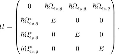
The Hamiltonian of the three-level quantum system, driven by an electromagnetic wave with the field-matter interaction of the system treated in the electric-dipole approximation, is described by H =Ha+ Σiµi·E(t), whereHais the Hamiltonian of

(35)

Figure 2.1: Schematic of the model three-level Λ system. The two transitions of the Λ are driven by the fields with Rabi frequencies Ω0 and Ω2 respectively.. The detuning

(36)

Hamiltonian can be written in the interaction picture as:

HRW A =

     

−_~40 ~Ω₂0 0

~Ω0

2 0 ~

Ω2

2

0 ~Ω2

2 −~41

      , (2.1)

where 4i represents the detuning between the incident field and the state transition

frequencies. The Rabi frequency, Ωi =µiEi, depends on the amplitude of the incident

electric field component parallel (Ei) to the dipole moment of the transition (µi).

In order to study the time-dependent response of the system to both the environ-ment and the incident electromagnetic wave, a density matrix representation of the system’s state is used. This density matrix ρij(i, j = 0,1,2) evolves in time according

to the Lindblad-von Neumann equation which takes the form:

˙ ρ=−i

~

[HRW A, ρ]−L(ρ). (2.2)

In this evolution equation, the Lindblad superoperator,L(ρ), models the decoherence in the system. This term is linear in the state density operator and is of the form:

L(ρ) = X

d=0,2 γd

2(σ

†

dσdρ+ρσ

†

dσd−2σdρσ

†

d). (2.3)

In this equation, σd are the Lindblad operators, and I assume that the only

de-coherence mechanism present is spontaneous emission. γd represents the decay or

In the case of general spontaneous emission between levels (|ii → |ji),

(37)

Using this operator, one can evaluate all the terms in the Lindblad superoperator:

σ_ij†σijρ=|ii hi|

"

X

a

X

b

ρab|ai hb|

#

=X

a

X

b

ρab|ii hb|δia, (2.5)

ρσ_ij†σij =

"

X

a

X

b

ρab|ai hb|

#

|ii hi|=X

a

X

b

ρab|ai hi|δib, (2.6)

σijρσ

†

ij =|ji hi|

"

X

a

X

b

ρab|ai hb|

#

|ii hj|=X

a

X

b

ρabδibδia|ji hj|. (2.7)

Combining all these terms, one can write down a general expression for matrix element Lmn for N total energy levels,

ˆ Lmn =

N

X

j

(γmj 2 +

γnj

2 )ρmn−2δmn

N

X

i

γin

2 ρii. (2.8)

To determine the fluorescence spectrum, I introduce a two-time correlation func-tion that evaluates the correlafunc-tion between the intensity being emitted from a transi-tion with lower level |ii at timet, with the intensity being emitted from a transition with lower level|jiat timet+τ. Using the quantum regression theorem [68], this cor-relation function is expressed in terms of the steady-state populations. A normalized, ensemble-averaged, correlation function is defined [68] as:

Gij(τ) =

h:Ii(t)Ij(t+τ) :i

h|ii hi|i h|ji hj|i , (2.9)

where h::i denotes time ordering. For the fluorescent transition |1i → |2i correlated to itself, this function takes the form [68]:

G22(τ) =

h:I2(t)I2(t+τ) :i

h|1i h1|i h|1i h1|i =

P2→1(τ) P1

, (2.10)

where P2→1(τ) represents the matrix element ρ11(τ) with initial condition ρ22(τ =

(38)

time t, the system has just emitted a photon from the |1i → |2i transition, resulting in ρ22(τ = 0) = 1, and the likelihood of the system to emit another photon in the

same transition (P2→1(τ) = ρ11(τ)) is tracked. From this correlation function, the

correlation spectrumG22(ω) can be determined via a Fourier transform. The results

of these spectra are then scaled to the Rabi frequency [see Appendix B].

2.3 Effect of Detuning on the Correlation

Spec-trum

When evaluating the time evolution of multi-level quantum systems, the state of the system oscillates with multiple frequencies due to the fact that coupled transitions interfere with one another. Therefore, in order to predict these couplings, one needs to look at the entire matrix interaction. These specific oscillations will only show up if two transitions are coupled by a common energy level.

If the system is in a nearly pure state, these oscillation frequencies can be predicted by looking at the eigenvalues (λj) and normalized eigenstates |φji(dressed states) of

the RWA Hamiltonian. This is due to the fact that if the decoherence is low (γd→0)

and the state is pure, the density matrix with the wavefunction in the eigenbasis can be expressed as:

ρ=|Ψi hΨ|=X

j,k

cjc∗kexp(−i(λj −λk)t/~)|φj(0)i hφk(0)|. (2.11)

If the RWA Hamiltonian is constant in time, the only possible time-dependent frequencies that can be seen are those that arise from the nonzero differences in the eigenvalues (λi) of the RWA Hamiltonian:

ωij =

X

j,k

(λj−λk)

(39)

While these are the only frequencies that are possible, it is also possible to not observe these oscillation frequencies if the eigenvector element of|φji or|φkiis zero.

For example if:

|φji=



    

0

1

√

2

1

√

2



    

, (2.13)

then no Rabi oscillation for frequencies involving λj will ever be seen in matrix

ele-mentsρ0iorρi0due to|φji hφk|having zero amplitude for that density matrix element.

The correlation spectrum of a three-level Λ system that has both transitions on resonance with an incident electromagnetic field will have a single peak observed at ω4=0 =

p

Ω2

0+ Ω22 [68]. This effect is understood by the presence of the zero-energy

“dark state” that does not couple to the excited fluorescing level. Thus, the only frequency observed in the correlation spectrum is that of the transition between the other two dressed states of the Hamiltonian. For the same reason, when a three-level Λ system is driven with both transitions at the same detuning (the so-called “two-photon resonance condition”), only a single peak will be observed in the correlation spectrum.

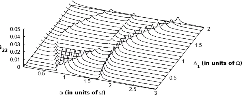
When the two detunings are not equal to each other (∆0 6= ∆1), there is no

dark state in the dressed state picture. Therefore I expect to see three peaks in the correlation spectrum as shown by the numerical calculations in Fig. 2.2. Detuning ∆0 is kept equal to Ω, while ∆1 is swept from zero to 2Ω. The three-peaked structure

of the correlation spectra changes to a single-peaked structure at the two-photon resonance condition ∆0 = ∆1 in which there is a zero eigenvector element.

(40)

Figure 2.2: Intensity-intensity correlation spectra for varying values of detuning 41

with Ω0 = Ω2 = Ω. The detuning40is kept fixed at a value of 1.0 Ω. The spontaneous

decay rate from the excited state is low with γ/Ω = 0.01.

λ3+ (40+41)λ2−(4041+

Ω2 0

4 + Ω2

2

4 )λ− 1 4(40Ω

2

2+41Ω20) = 0. (2.14)

The differences between the eigenvalues of the dressed Hamiltonian determines the location of the peaks in the correlation spectrum. Since the equation is cubic, there are three eigenstates. Transitions between all three pairs of eigenstates are allowed, hence it is possible to observe three peaks if there exists a non-equal detuning of both transitions. In the case of equal detuning, the presence of a dark state (eigenvector with a zero element) prevents the three-peaks from being observed, and only one peak is observed.

The deterministic location of the peaks in the correlation spectra as a function of the two detunings suggests a practical application. If the peak frequencies in the two-time intensity-intensity correlation spectrum are measured, those peak frequencies can be used to infer whether transitions are connected and extract the values of both detunings if one knows the strengths of the Rabi frequencies of each transition.

(41)

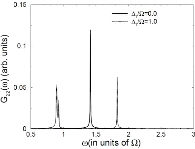
Figure 2.3: Intensity-intensity correlation spectra of a fluorescent transition in a Λ system for various values of 41 for 40 = 0. Both transitions are driven by the same

Rabi frequency Ω. The rate of spontaneous decay is low with γ <<Ω.

that Ω0 = Ω2 = Ω and 40 = 0, but ∆1 can change away from 0. If one of the

detunings (say ∆0) is on resonance, and the other detuning (∆1) is not, I expect to

see the three peaks in the correlation spectrum shown by numerical calculations in Fig. 2.3. To estimate the positions of the spectral peaks, Eq. 2.14 is simplified to:

λ3+ (41)λ2−(

Ω2 2 )λ−

Ω2

4 (41) = 0 (2.15)

and the differences in the dressed state eigenenergies are calculated.

If41 = 0, thenλ1 =−√Ω₂,λ2 = 0 andλ3 = √Ω₂ and the corresponding eigenvectors

are |φ1i = (1,−

√

2,1), |φ2i = (−1,0,1) and |φ3i = (1,−

√

(42)

and ω13 = |λ1 −λ3| =

√

2Ω. However in G22(τ), which depends on density matrix

element ρ11, ω12 and ω23 will not show up in the spectrum because |φ2i contains a

zero component for |1i. This yields a single peak in Fig. 2.3.

If 41 = 1, then λ1 ≈ −1.2406Ω, λ2 ≈ 0.5850Ω and λ3 ≈ −0.3444Ω and the

corresponding eigenvectors are |φ1i ≈(0.1939,−0.4811,1), |φ2i ≈(2.7092,3.1700,1)

and |φ3i ≈ (−1.9032,1.3111,1). Therefore the allowed possible real frequencies are ω12=|λ1−λ2|= 1.8256Ω,ω23 =|λ2−λ3|= 0.9294Ω andω13 =|λ1−λ3|= 0.8962Ω.

As none of the eignevectors contains zero elements, all three interference peaks will be observed. This yields the triple peak structure in Fig. 2.3.

If the time dependance of G22 is measured in an experimental system, and the

frequencies in the signals extracted, the detuning41 can then be calculated in units

of the Rabi frequency Ω.

2.4 Effect of Spontaneous Emission on the

Corre-lation Spectrum

The above discussion and analytic results are based on the assumption that sponta-neous decay processes are small in magnitude relative to the driven Rabi oscillations, and do not contribute significantly to the observed spectra. However, for most real systems, spontaneous decay is present and may impact the spectra that can be ob-served. Previous work on resonantly-driven 3-level ladder systems [68] has shown that the presence of significantly strong decay can modify the observed spectra by the inclusion of additional peaks. Therefore I investigate how spontaneous decay can affect the observed intensity spectra in ournon-resonantly driven, 3-level Λ system.

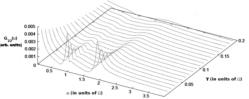
For the example system in which Ω01 = Ω12 = Ω and 40 = 0, assuming that

(43)

Figure 2.4: Intensity-intensity correlation spectra for increasing amounts of sponta-neous decay γ with fixed detuning41 = Ω₂, and 40 = 0. As the rate of spontaneous

decay increases, the peaks broaden and become less distinguishable.

the three-level ladder system [68]. In fact, under low amounts of spontaneous decay, the transitions observed are the same as those analytically predicted from Eq.2.14. However, when the decay becomes significantly strong, I observe a broadening in the correlation peaks which may obscure or merge some peaks that are closely spaced. In addition, the high rate of spontaneous decay can also obscure correlation peaks that are at low frequencies due to the system quickly reaching a steady state.

These effects can be seen in the plots below in Fig. 2.4 in which the intensity-correlation spectra are plotted for varying amounts of spontaneous decay. In all cases, the presence of significant decay serves to broaden the peaks observed. For the case of fairly high decay (γ/Ω = 0.10), the inclusion of this decay broadens the peaks to a point at which only two of the three peaks are visible.

2.5 Effect of Dephasing on the Correlation

Spec-trum

(44)

Figure 2.5: Intensity-intensity correlation spectra for increasing amounts of dephasing δd = δ0 = δ2 with fixed detuning 41 = Ω₂, and 40 = 0 as well as fixed spontaneous

decay (γ = 0.01Ω) . As the rate of spontaneous decay increases, the peaks broaden and become less distinguishable.

two-time correlation spectra. In order to examine this, dephasing elements are added to the Lindblad matrix of the form:

Ld=



    

0 δ0ρ01 (δ0+δ2)ρ02 δ0ρ10 0 δ2ρ12

(δ0+δ2)ρ20 δ2ρ21 0



    

, (2.16)

where δi is the dephasing of the transition with ground state |ii. If I take a look

at the case in which the two dephasings are equal, I observe that the main effect of dephasing is similar to that of high spontaneous decay. By including dephasing in my calculations, the peaks in the spectra are broadened.

2.6 Potential Application of this Method

(45)

level structure of a complex atom directly. If a pair of transitions is driven, quantum interference effects will only be present if the two levels share a common state. This effect is useful as it is an interaction that can be observed experimentally with no need to understand the underlying properties of the states in question.

As the overall process is time-dependent, it could also form the basis for an in-teraction detection method. If the two-time intensity-intensity correlation spectrum were to be continuously monitored for a target transition in a three-level system, any changes that occur in the spectrum could be used to determine if any of the energy levels have changed in real time. This would indicate that an interaction has taken place, although there are many alternate ways of doing this [70, 71]. The position of the peak frequencies can then be used to extract the detuning/level shift informa-tion from the map of the expected peak frequencies in the correlainforma-tion spectra due to differing amounts of detuning in both levels.

(46)

2.7 Summary

In this section, I have examined the control of a single open quantum system. For this system, the state of the atom/molecule evolves directly according to the Lindblad-Von Neumann master equation. Although an exact analytic solution for the quantum states is not available, one can analytically predict both the steady-state of these dense systems as well as the oscillating frequencies of the states.

(47)

Chapter 3 Quantum Behaviour with a

Classical Environment

3.1 Motivation - Improving Qubit Preparation/Cooling

Times

The practical implementation of quantum computers [28] places two specific require-ments on the lifetime of a quantum bit or a qubit, namely, long relevant decoherence times, and rapid state initialization times. A great deal of recent research has been de-voted to proposing solutions that minimize the overall spontaneous emission rate and preserve system purity[29, 30, 31, 32, 33]. These decoherence-minimization processes lead to longer effective qubit operational lifetimes, but decoherence will ultimately render the qubit unusable due to loss of state purity. The simplest way to restore system purity is to wait for the system to cool to a pure state, usually the ground state.

(48)

timescales of the control processes; i.e., the spontaneous emission rate is selected to be quite low. Thus, the desires for long operational times and short cooling times of a qubit place contradictory demands on the spontaneous emission rate of the quantum excited state. There is a need for protocols wherein the spontaneous emission rate of a quantum system can be selectively decreased so that long state lifetimes can be maintained during operation, and upon demand, selectively increased so that the cooling time can be drastically shortened in duration when qubit purity needs to be restored.

Recent experiments have increased the spontaneous emission rate of a quantum excited state by coupling the system to a nearby resonant structure such as a cavity [42, 43, 44, 45, 72], photonic crystal [46] or nanoparticle [72] based on the Purcell effect [73]. However, these studies have not been able to toggle a system between a configuration where the spontaneous emission rate is low (for qubit operation) and high (for qubit initialization).

(49)

3.1.1 Description of a Classical Environment

In what I call a classical environment, local structures that modify electromagnetic fields are present, but they interact with electromagnetic fields either as classical dipoles or by having a bulk index of refraction. In this type of environment, one can also assume that the environmental elements have no state memory, and do not display any quantum properties (such as electromagnetically induced transparency, spontaneous emission or quantum interference between levels).

I also assume that the state of the quantum system does not significantly affect local field intensities. This allows for the separation of the overall control calculations into two separate parts: a classical field propagation calculation, and a quantum evolution calculation.

The electromagnetic field calculations involve determining how fields propagate through the environment, and how strongly the dipole transitions present in the quantum system couple to this environment. These couplings allow us to modify our control fields and decoherence rates with constant enhancement factors [34]. As these control parameters are modified by the external environment, the input parameters of the quantum control calculation are also modified. In addition, the specific type of environment I choose to examine (noble metal nanoparticles) acts as a resonator with respect to the quantum system. The specific properties of this resonator depend on its size, shape and composition.

3.1.2 Effect of a Noble-Metal Nanoparticle on a Quantum

System

(50)

sub-wavelength in size, the atomic electrons located inside them are able to collec-tively oscillate in phase with one another. This collective oscillation, referred to as a localized surface plasmon oscillation, leads to greatly enhanced local electric field intensities and strong decay modes being created around the nanoparticles at specific resonance frequencies [77]. Localized surface plasmon resonance (LSPR) is a common detection technique that uses this effect to evaluate adsorption of various objects onto nanoscale surfaces by looking for changes in this resonance [78, 79].

When a noble metal nanoparticle is illuminated by a broadband electromagnetic field, the evanescent field around the metal surface is intensified at the localized surface plasmon wavelength [80]. When a dipole emitter is placed near noble-metal nanoparticle, the rate of dipole emission is enhanced due to the Purcell effect [73, 34, 35]. Thus when a noble-metal nanoparticle is placed near a resonantly-driven quantum system, one expects the control field and the spontaneous emission rate to be enhanced.

Of these two principal types of enhancement, the enhancement to the decoherence rate is much more important in quantum control than the enhancement of the fields. This is due to the fact that field intensities are external to the quantum system itself; field enhancement can always be accounted for by adjusting the incident intensity. However, the decoherence rate enhancement is usually intrinsic to the system itself and is much harder to adjust.

(51)

compromising qubit fidelity.

3.2 Theoretical Methodology

3.2.1 Electromagnetic Field Propagation

The propagation of fields through these environmental structures are evaluated by solving Maxwell’s equations numerically. Although various techniques exist for solv-ing this problem on the nanoscale, such as the discrete-dipole approximations (DDA) [81], Mie theory [82] and diffraction optics, [83], in the time-domain one directly solves Maxwell’s equations. As this solution involves calculating a propagation in time as well as space, this involves concurrently solving the Maxwell-Faraday equation and Ampere’s law in differential form,

∇ ×E=−µ∂H

∂t , (3.1)

and

∇ ×H=∂E

∂t +σE+J. (3.2)

In this work, a robust commercial solver (Lumerical [84]) has been used to calculate the field evolution; this particular software operates using a finite-difference time domain (FDTD) method. This method uses finite differences to evaluate spatial derivatives.

(52)

Green’s theorem [85, 86, 87] or Mie theory [82].

After the fields have been propagated through the environmental geometry, the electric fields are recorded at various real-space coordinates.

3.2.2 Electromagnetic Field Enhancement Around a Silver

Nanoparticle

The LSPR effect can be seen in Figure 3.1. Around noble-metal nanoparticles, there is an enhanced field intensity due to the strong interaction between the incident field and electrons in the metal particles. For these spherical metal nanoparticles, the strongest field enhancement is along the polarization direction of the driving field and exists in a dipole pattern. This enhancement is qualitatively similar to the increased electric field enhancement that can be determined analytically by determining the electric field distribution around a perfectly conducting nanosphere using a method of images and a constant input field [88]. This similarity is due to both the high conductivity of the noble-metals as well as the fact that, at the nanoscale, the entire metal nanosphere experiences roughly the same electric field (i.e., the dipole approximation is valid).

(53)

Figure 3.1: An xy plot of electric field intensities (|E| at 475 nm) for a ˆy polarizaed wave travelling in the ˆz direction around a 20 nm Ag nanoparticle.

together. Tuning such an arrangement could be as simple as placing pairs of particles differing distances apart [75]. Depending on the particle’s properties and the pair’s inter-particle spacing, this arrangement could have an even greater effect on the field enhancement around the nanoparticle array than a single particle [36].

The relatively high degree of tunability of these nanoplasmonic systems allows them to be easily adopted to enhance most quantum systems that have transitions in the optical range. This enhancement is also well-documented due to the use of nanoplamsonics in enhancing solar cell efficiencies [90] and in surface binding detectors [75].

3.2.3 Decay Rate Enhancement Around a Ag Nanoparticle

(54)

(55)

γd,f ree =

ω3 0|µ|2

3π0~c3 = ω

3

0| hg|µˆ|ei |2

3π0~c3

, (3.3)

where ωo is the frequency of the transition and µ is transition dipole moment. This

equation assumes that the driving fields are on resonance with the transition, the fields and decay rates are constant at all times and that the system is decoupled from its environment.

However, when dealing with a system that can couple to external modes, it is possible to modify this decay by assuming that the transitions in the system behave as radiating electric dipoles. In this case, an approximate modified decay rate can be calculated by comparing the power that is emitted from the system in its environment, as compared to that same system in free space [34, 21]. Thus, the new decay rate can be determined by [21],

Md=

γd

γd,f ree

= P ower P owerf ree

. (3.4)

In a classical environment, it is assumed that the transitions behave like classical dipoles at all times. In this case, the transition can be modelled as an oscillating electric dipole source, of frequencyω, and placed into the environment. The coupling of this source to nearby environmental objects is then calculated to find the power emitted by the transition [34, 35]. In the FDTD solver, this can be done by defining a 3D surface enclosing just the dipole, and by calculating the Poynting vector along the surface:

S(r, ω) = 1 µ0

E(r, ω)×B(r, ω). (3.5)

(56)

P ower =

‹

A

S(r, ω)·dA. (3.6)

This power emission is then compared to the power emission of a classical dipole to determine the decay enhancement factor, as a function of frequency, using Equation 3.4. This effect of a proximate noble-metal nanoparticle was used to examine the possibility of surface-enhanced state purification with two-level systems and details of that investigation (and its inherent limitations) are included in Appendix C.

The fact that the decay enhancement is dependent on the dot product (µ·E) indicates that the polarization of the transition dipole of a driven state can be used to selectively enhance its decoherence rate. This effect should allow for polarization control of decoherence if the system is placed next to an asymmetric environment. I will therefore use this to propose a system in which rapid state preparation can be achieved in conjunction with high qubit fidelity.

3.3 Control of a Quantum System between two

Sil-ver Nanoparticles

(57)

strongly frequency dependent, thus applied to surface-enhanced fluorescence [91, 35]. It is less well-known that the modification of the spontaneous emission rate due to the weak coupling to the surface plasmon modes exhibits a strong dependence on the polarization of the incident light [21, 92]. In the scheme I describe below, changing the polarization direction of the electromagnetic wave from perpendicular-to-the-interparticle-axis to parallel-perpendicular-to-the-interparticle-axis changes the spontaneous emission rate of a quantum emitter at a particular wavelength from very low to very high. This effect can be used to develop a protocol wherein one of the arms of a three-level Λ system (3LLS) can be used as a qubit that has a long coherence life-time during the operational mode, and quickly reset to a pure state when the qubit becomes unusable due to decoherence.

In my calculations, a radiating dipole (modelling a quantum dipole transition in a qubit) is placed equidistantly between two spherical Ag nanoparticles, of radius r and surface-to-surface separation d as shown in the inset in Fig. 3.3a). The res-onance spectra of these NPs can be tuned by changing their size and composition [93], allowing for a wide variety of quantum systems to be used as a qubit platform. I assume that the dipole is oriented by the polarization of an electromagnetic wave that illuminates the nanoparticles. I examine two cases — firstly when the dipole is oriented perpendicular to the interparticle axis (ˆz), and secondly when the dipole is oriented parallel to the interparticle axis (ˆx).

(58)

transition frequency of the qubit. This frequency is similar to transition frequencies found in ultraviolet quantum dots such as ZnO [94] and due to the tunability of both the nanoparticle resonance and the qubit energy level spacing, such a frequency choice serves as a good model to illustrate how polarization control can speed up qubit initialization. I also assume that these systems have no inherent preferred quantization axis.

The local electromagnetic field vector components (Ex, Ey, Ez) at the location of

the quantum emitter (halfway in between the nanoparticles on the interparticle axis) due to the driving fields are calculated numerically by solving Maxwell’s equations for different incident field polarizations. A commercial-grade simulator based on the finite-difference time domain method was used to preform the calculations [84]. The optical response of the material is determined by fitting the Drude model using experimental constants [89]. The magnitude of the incident electric field is assumed to beE0 in both polarizations. I define a “field enhancement factor”ME,i =|Ei|/E0,

distinct from the intensity magnification factors usually reported in studies of surface-enhanced processes. Figure 3.3(a) shows the field enhancement factors in the ˆz (blue, solid line) and ˆx (red, dashed line) components of the field when the incident light is polarized in the same (ˆz or ˆx) direction. These two curves show that the presence of the nanoparticles greatly enhances the field strength in the direction of polarization of the incident light. Thus, the driven qubit is driven much harder (or the Rabi frequency increases) due to the presence of the proximate nanoparticles.

The rate of spontaneous emission of the quantum emitter changes when placed in between the two AgNPs. This change in the rate of spontaneous emission is cal-culated by modelling the quantum emitter as a point oscillating dipole source. I compare the power emitted by the point dipole source with (PN P), and without the

nanoparticles (PN oN P) [34] by solving Maxwell’s equations numerically [84]. The

(59)

Figure 3.3: (a) Field enhancements (ME,i=|Ei|/E0) and (b) decay rate modification

(60)

around the dipole source. This decay enhancement factor is also the ratio of the spontaneous emission rate of the dipole emitter with the nanoparticles γ to the vac-uum spontaneous emission rate γ0 [21]. The decay enhancement factor as a function

of wavelength is evaluated for two different orientations of the dipole; one in which the dipole is perpendicular to the interparticle axis (ˆz) and the other in which it is parallel to the interparticle axis (ˆx), and presented in Fig.3.3(b). I see that at wave-lengths near the qubit resonance, the rate of spontaneous emission of the quantum emitter can be increased by switching from z to xpolarization.

Thus the polarization of the driving field both modifies the Rabi frequency and the spontaneous decay rate of the qubit transition parallel to it. Based on the above analysis, the wavelength of the incident electromagnetic wave is chosen so that the ratio of parallel decay rate (γx) to the perpendicular decay rate (γz) is maximized

(≈420 nm).

For a practical qubit implementation, I offer the following protocol:

Step 1: Consider a three-level quantum system in the ‘lambda’-configuration (3LLS), with both ground states |gi and |ci being somewhat close in energy though not degenerate. The lifetime of the excited state |ei is long enough for the quantum system to be a good candidate for quantum information processing. This system can then be placed in between two silver nanoparticles. The two ground states, |gi and

|ci, are chosen as the qubit, and gate operations are carried out by a near-resonant

electromagnetic wave polarized in the ˆz-direction — perpendicular to the interparticle axis. This allows the rate of spontaneous emission from the excited states, γge,z and

γce,z, to remain fairly low. Without loss of generality, one can assume that the ground

states are angular momentum j = 0 states, and the excited state is a j = 1 state, thus the applied linearly polarized field transitively connects the |g, j = 0, m = 0i

state with the |e, j = 1, m= 0istate.

(61)

to be initialized, the polarization of the incident electromagnetic wave is rotated by 45◦ to excite both along the ˆz and ˆx directions. Polarization selection rules create a five-level system transitively connected as shown in Fig. 3.4. Thez-polarized compo-nents continue to connect the |g, j = 0, m = 0i and |c, j = 0, m = 0i states with the

|e, j = 1, m= 0istate, and the spontaneous emission stays low (blue, solid lines). The

x-polarized components connect the|g, j = 0, m= 0istate and|c, j = 0, m= 0iwith the|e, j = 1, m=±1istates, and the spontaneous emission from the latter states are high (red, dashed lines).

If the detunings of both transitions are kept equal ∆ge = ∆ce, a Morris-Shore [95, 96]

transformation shows that these transition dipole couplings put the 3LLS into a dark state [97, 98], i.e., a superposition of the two ground states of the five-level system, which is a pure state. Thus, regardless of the initial quantum state of the system, the state can be rapidly reset into a pure state, i.e. the dark state.

Step 3: The rest of the qubit initialization can be completed by rotating the po-larizations of the two electromagnetic waves perpendicular to the interparticle axis. In this configuration, the spontaneous emission from the excited state|ei is low, and population can be transferred coherently to the qubit ground state |gi.

(62)

Figure 3.4: Polarization control scheme for rapid qubit initialization. Two applied fields near resonant with the|gi-|eiand |ci-|ei transitions are linearly polarized in thex−z plane. Thezcomponents of the field excite the blue (solid) transitions, while thexcomponents of the field excite the red (dashed) transitions. For preparation, the Rabi frequencies of all transitions are high with respect to spontaneous decay rates. The spontaneous emission rates of the operational (blue, solid) transitions, γge,z and

γce,z, stay low, whereas those of the preparation transitions (red, dashed), γge,x, and

γce,x, are greatly enhanced. The detunings are chosen to coherently trap the system

Quantum Control of Open Systems and Dense Atomic Ensembles

Scholarship at UWindsor

Scholarship at UWindsor

Quantum Control of Open Systems and Dense Atomic Ensembles

Quantum Control of Open Systems and Dense Atomic Ensembles

Quantum Control of Open Systems and Dense Atomic

Ensembles

Quantum Control of Open Systems and Dense Atomic

Ensembles

Declaration of Previous Publication

Abstract

Acknowledgements

Contents

List of Figures

Glossary of Symbols

Chapter 1

Introduction

1.1

Dissertation Overview

1.1.1

Control of a Single, Open Quantum System

1.1.2

Control of an Open Quantum System Interacting with

a Nearby Classical System

1.1.3

Evolution of Dense Quantum Ensembles

1.1.4

Effective Single Particle Model of the Evolution of a

Dense Quantum Ensemble

1.1.5

Appendices

Chapter 2

Control of an Individual, Open

Quantum System

2.1

Spectroscopic Detection of Couplings Between

State Transitions

2.2

Theoretical Model

2.3

Effect of Detuning on the Correlation

Spec-trum

2.4

Effect of Spontaneous Emission on the

Corre-lation Spectrum

2.5

Effect of Dephasing on the Correlation

Spec-trum

2.6

Potential Application of this Method

2.7

Summary

Chapter 3

Quantum Behaviour with a

Classical Environment

3.1

Motivation - Improving Qubit Preparation/Cooling

Times

3.1.1

Description of a Classical Environment

3.1.2

Effect of a Noble-Metal Nanoparticle on a Quantum

System

3.2

Theoretical Methodology

3.2.1

Electromagnetic Field Propagation

3.2.2

Electromagnetic Field Enhancement Around a Silver

Nanoparticle

3.2.3

Decay Rate Enhancement Around a Ag Nanoparticle

3.3

Control of a Quantum System between two

Sil-ver Nanoparticles