ABSTRACT
PARSONS, GREGORY S. Dynamic Frequency and Voltage Scaling Rivalrous Real-time Embedded Systems. (Under the direction of Dr. Alexander G. Dean.)
Some embedded real-time systems have hardware elements that naturally interfere with each other, preventing their simultanious use. The primary example studied in this thesis, among others, is that of a switch-mode power supply (SMPS) driving a Dynamic Voltage and Frequency Scaling (DVFS) embedded system containing other hardware elements which, by either necessity or design, are prone to suffer interference. In this configuration, these hardware elements can be considered rivalrous, an economics term for goods which cannot be used correctly by more than one entity at a time. However, thanks to our deployment of Rivalrous Hardware Scheduling (RHS) which allows the application of real-time scheduling techniques to rivalrous hardware tasks, we can allow the temporal isolation of otherwise incompatible (e.g. noise-generating and noise-sensitive) tasks without interference, all the while minimize energy consumption and satisfying hard realtime deadlines. We demonstrate these proposed scheduling techniques and other concepts by building them into several embedded platforms, including underwater communication and down-well communication.
Another contribution of this dissertation is to demonstrate various novel benefits from build-ing up the walls of abstraction between embedded system hardware and software through the use of automated code and scheduling analysis. This abstraction allows the deployment of various stages of automated code design, bridging the gap between the need for embedded systems and the difficulty in their design. To this end, we have developed new methods and implemented them in various tools enabling the rapid prototyping of various stages of embed-ded systems design. One such tool is the RaPTEX toolchain, which allows users to utilize the modular interface to simplify the creation of new custom applications, alleviating the need for high-level user design decisions, which can be handled by the toolchain.
Dynamic Frequency and Voltage Scaling Rivalrous Real-time Embedded Systems
by
Gregory S. Parsons
A dissertation submitted to the Graduate Faculty of North Carolina State University
in partial fulfillment of the requirements for the Degree of
Doctor of Philosophy
Computer Engineering
Raleigh, North Carolina
2013
APPROVED BY:
Dr. Eric Rotenberg Dr. Vincent W. Freeh
Dr. James M. Tuck Dr. Alexander G. Dean
BIOGRAPHY
Gregory S. Parsons was born in his home town of Fayetteville, North Carolina in the year 1980. He moved to the dormitories of North Carolina State University in the Fall of 1998 and received his Magna cum Laude Bachelors of Science and Masters of Science degrees in Computer Engineering in 2002 and 2003, respectively. He transitioned to pursue his Ph.D. degree in 2003 under the advisory of Dr. Alexander G. Dean in what was at the time called the Center for Embedded Systems Research (CESR). His research continues to focus on embedded systems design and optimization.
Gregory Parsons was certified as an Engineering Intern (EI) in the State of North Carolina in 2003.
ACKNOWLEDGEMENTS
My greatest appreciation goes to my advisor and mentor, Dr. Alexander G. Dean, for his mentorship and ability to maintain good humor in the face of adversity. If not for his guidance, and especially patience, this dissertation would most certainly not exist. Thank you, Master Dean!
I would also like to thank my other advisory committee members, Dr. Eric Rotenberg, Dr. Vincent W. Freeh, and Dr. James M. Tuck, for forcing a necessary course correction in my research and valuable feedback on my dissertation. My thanks also go to all the other professors in the ECE department who enriched my time here at North Carolina State University and ultimately put me on this path.
I must also mention my colleagues in what is now the Center for Efficient, Scalable and Reliable Computing (CESR), Dr. Won So, Zane Purvis, Dr. Shaolin Peng, Sangyeol Kang, Karthik Sundaramoorthy, Dr. Rony Ghattas, Avik Juneja, Linda Fontes, Subash Sachidananda, and Adarsh Seetharam, for their comradery in the face of academia, and all the help they provided. I would like to especially thank Shaolin Peng for his long collaboration on the projects and contributions of this dissertation and his continuing friendship.
TABLE OF CONTENTS
LIST OF TABLES . . . vii
LIST OF FIGURES . . . .viii
Chapter 1 Introduction . . . 1
1.1 Motivation . . . 1
1.2 Contributions . . . 1
1.2.1 Projects . . . 2
1.2.2 Real-Time Scheduling . . . 2
1.2.3 Automated Tool Design . . . 2
1.2.4 Communication Systems . . . 4
1.3 Publications . . . 5
1.4 Document Outline . . . 7
Chapter 2 Rivalrous Hardware Scheduling (RHS) . . . 8
2.1 Motivation . . . 8
2.1.1 Alternatives to Scheduling . . . 10
2.2 Contributions . . . 10
2.3 Deployed Examples of RHS . . . 11
2.3.1 Underwater Communication . . . 11
2.3.2 Downwell Communication . . . 13
2.4 Prior Work . . . 14
2.4.1 Energy Aware Scheduling . . . 14
2.4.2 DVS and DFS Aware Scheduling . . . 15
2.4.3 Handling of Scheduling Complexity . . . 15
2.4.4 Scheduling with a Rivalrous Power Supply . . . 16
2.5 System Description . . . 16
2.5.1 Scheduling Paradigm . . . 16
2.5.2 Power Model . . . 17
2.6 Evaluated Scheduling Approaches . . . 19
2.6.1 Online Scheduling . . . 20
2.6.2 Quasi-Static Scheduler . . . 20
2.6.3 Schedule Building . . . 20
2.7 Scheduler Evaluation . . . 24
2.7.1 Synthetic Task Set . . . 24
2.7.2 Quasi-Static Versus Online Scheduling . . . 25
2.7.3 Quasi-Static Scheduler Aided Hardware Design . . . 29
2.8 Laboratory Deployment . . . 30
2.8.1 Rivalrous Hardware . . . 31
2.8.2 Quasi-Static Scheduling . . . 31
2.9 Conclusions . . . 36
Chapter 3 Unified Replay Environment . . . 37
3.1 Related Work . . . 38
3.1.1 Input Recording and Replay . . . 38
3.1.2 Embedded Benchmarks . . . 40
3.2 Methods . . . 41
3.2.1 Language Selection . . . 42
3.2.2 Event Description Storage . . . 42
3.2.3 Event Classification . . . 43
3.2.4 Time Subsystem . . . 43
3.2.5 Input Operations . . . 44
3.2.6 Interrupts . . . 44
3.2.7 Application Program Interface . . . 44
3.2.8 External Timing Harness . . . 45
3.3 Experiments . . . 45
3.3.1 Target System . . . 45
3.3.2 Record and Replay Procedures . . . 46
3.3.3 Microcontrollers . . . 46
3.3.4 Sample Programs Evaluated . . . 48
3.4 Results . . . 49
3.4.1 Performance Variations with Clock Rate . . . 49
3.4.2 Performance Across Architectures . . . 50
3.5 Conclusions . . . 52
Chapter 4 RaPTEX . . . 53
4.1 RaPTEX Internals . . . 54
4.1.1 Application Decomposition . . . 54
4.1.2 Module Integration . . . 54
4.1.3 XMDL Abstraction . . . 56
4.1.4 Toolchain Execution . . . 56
4.1.5 Graphical User Interface . . . 57
4.2 Code Generation . . . 58
4.3 Code Analysis . . . 58
4.4 User Experience . . . 58
4.5 Demonstration . . . 60
4.5.1 Transmitter . . . 61
4.5.2 Receiver . . . 64
Chapter 5 Underwater Communication System Design . . . 68
5.1 Phase I . . . 70
5.2 Phase II . . . 72
5.2.1 Packet Processing . . . 75
5.2.2 Performance . . . 76
5.2.4 Receiver Power Consumption . . . 78
5.2.5 Range Evaluation . . . 79
5.3 Phase III . . . 79
5.4 Simulator Overview . . . 80
5.5 Experiment & Simulation Results . . . 80
5.5.1 Offered Load Effects . . . 81
5.5.2 Channel Noise Effects . . . 83
5.5.3 Network Size Effects . . . 85
Chapter 6 Downwell Communication . . . 87
6.1 Introduction . . . 87
6.2 Contributions . . . 88
6.3 Challenges . . . 88
6.3.1 Attenuation . . . 88
6.3.2 Interference . . . 89
6.3.3 Protocol Design . . . 89
6.4 Application Environment . . . 90
6.5 Communication Platform Overview . . . 93
6.6 Phase IV . . . 94
6.7 Phase V . . . 96
6.7.1 Software . . . 98
6.8 Rig Floor Test Results . . . 105
6.8.1 Phase III Results . . . 105
6.8.2 Phase IV Results . . . 106
6.8.3 Phase V Results . . . 109
6.8.4 Phase 6 Test . . . 113
6.9 Conclusions . . . 118
Chapter 7 Conclusions. . . .119
LIST OF TABLES
Table 2.1 System Tasks and Rivalrous Resource Conflicts . . . 33
Table 3.1 Microcontroller Overview . . . 47
Table 3.2 Compilers Used . . . 47
Table 3.3 Application Characteristics . . . 48
Table 3.4 Stimulus Characteristics . . . 49
LIST OF FIGURES
Figure 2.1 Oscilloscope Trace of System Utilizing RHS and QSS . . . 9
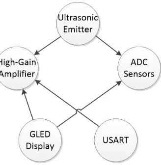
Figure 2.2 Rivalrous Resources Conflict Diagram for Underwater Transceiver . . . . 12
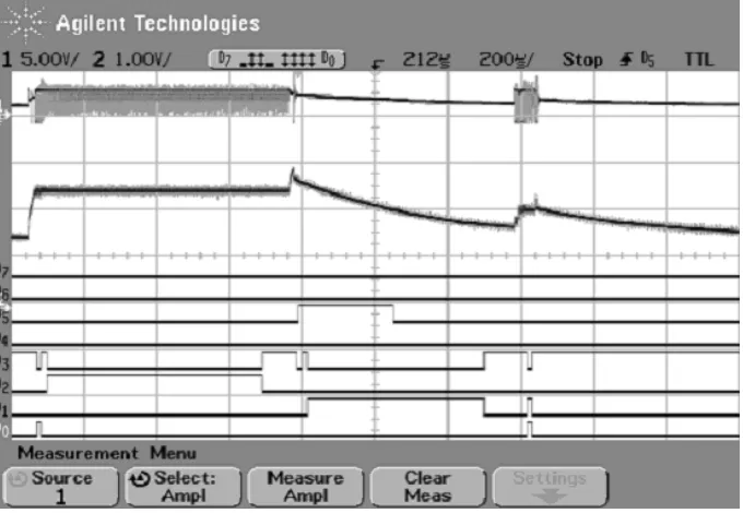
Figure 2.3 Interference between external crystal oscillator (bottom) and high-gain Amplifier (top) . . . 12
Figure 2.4 Interference between GLED Display (bottom) and high-gain Amplifier (top) . . . 13
Figure 2.5 Cross-Pin Interference between the UART (bottom) and high-gain Am-plifier (top) . . . 13
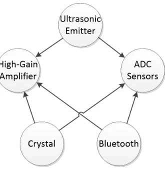
Figure 2.6 Rivalrous Resources Conflict Diagram for Downwell Transceiver . . . 14
Figure 2.7 Power-rail disruption from delayed bluetooth transmission . . . 15
Figure 2.8 Hardware Model Schematic . . . 17
Figure 2.9 Mathematical Hardware Model . . . 19
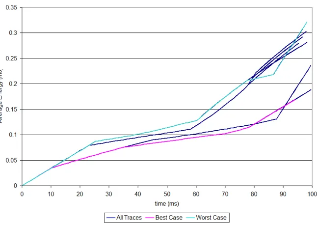
Figure 2.10 Sample Graphing of All Profiled Executions of Synthetic Task Set . . . . 23
Figure 2.11 Time required to build a complete quasi-static schedule versus complexity 23 Figure 2.12 Conflict Graph of Simulation Tasks . . . 24
Figure 2.13 Rivalrous, Execution Traces of QSS vs. GETF at 98ms period, or 40% Util. . . 25
Figure 2.14 Quasi-Static Scheduler Switching Points Command-Line Output - offline Scheduler (left) GETF online Scheduler (right) - Graphical version can be seen in Figure 2.13 . . . 26
Figure 2.15 Non-Rivalrous Performance Comparison of QSS vs. a range of online Schedulers . . . 27
Figure 2.16 Rivalrous Performance Comparison of QSS vs. a range of online Schedulers 27 Figure 2.17 Performance Comparison of QSS vs. the best online Scheduler . . . 28
Figure 2.18 Non-Rivalrous Performance Comparison of QSS vs SETF at 98% & 70% Util. . . 29
Figure 2.19 Design Space Exploration of the Power Supply Module for a fixed task set 30 Figure 2.20 MCU Integrated Power Supply Module . . . 31
Figure 2.21 Rivalrous Resources . . . 32
Figure 2.22 Rivalrous Resources Conflict Diagram . . . 33
Figure 2.23 Target Hardware Timing Harness Profile Data . . . 34
Figure 2.24 Oscilloscope Trace of System Utilizing RHS and QSS . . . 35
Figure 3.1 Overview of RE approach . . . 42
Figure 3.2 Normalized AVR Clock Scaling . . . 50
Figure 3.3 Normalized Platform Execution Times . . . 51
Figure 3.4 Power Consumption . . . 51
Figure 4.1 Overview of RaPTEX Software Toolchain . . . 53
Figure 4.2 XML Module . . . 55
Figure 4.4 Debugging Window . . . 59
Figure 4.5 Performance Window . . . 59
Figure 4.6 Transmitter Hamming ETH Results . . . 62
Figure 4.7 Transmitter Timing Results . . . 63
Figure 4.8 Transmitter Energy Consumption per Packet . . . 63
Figure 4.9 Transmitter Memory Results . . . 64
Figure 4.10 Basic Receiver Timing Results . . . 65
Figure 4.11 MinDig Receiver Variant Timing Results . . . 66
Figure 4.12 Receiver Schedulability . . . 67
Figure 4.13 Receiver Memory Results . . . 67
Figure 5.1 Phase I PCB Layout of the Receiver . . . 70
Figure 5.2 Phase I PCB Layout of the Transmitter . . . 70
Figure 5.3 Phase I Receiver (left) and Transmitter (right) . . . 71
Figure 5.4 Transducer . . . 71
Figure 5.5 Schematic of the Transducer Driver . . . 72
Figure 5.6 Voltage across Transducer, voltage to Q1, at Startup . . . 73
Figure 5.7 Voltage across Transducer, voltage to Q1, shifting frequency . . . 73
Figure 5.8 Voltage across Transducer, voltage to Q1, at Shutdown . . . 74
Figure 5.9 Phase II Transmitter Design . . . 75
Figure 5.10 Phase II Receiver Design . . . 76
Figure 5.11 Percent of Error Free Packets at 30 meters . . . 77
Figure 5.12 Transmitter Board Current Draw at 2.8V . . . 77
Figure 5.13 Battery life of CR2450 Lithium at 42 baud . . . 78
Figure 5.14 Range Testing Environment - Test1 at 30 meters and Test2 at 100 meters 79 Figure 5.15 Transducer without Display . . . 80
Figure 5.16 Discrete Event Network Simulator Overview . . . 81
Figure 5.17 CSMA performance vs. offered load . . . 82
Figure 5.18 MACA performance vs. offered load . . . 83
Figure 5.19 CSMA performance vs. channel noise . . . 84
Figure 5.20 MACA performance vs. channel noise . . . 85
Figure 5.21 CSMA performance vs. spatial network size . . . 86
Figure 5.22 MACA performance vs. spatial network size . . . 86
Figure 6.1 Drilling field . . . 90
Figure 6.2 Drilling Pipe . . . 91
Figure 6.3 Pipe Chamber . . . 92
Figure 6.4 Drilling Platform Overview . . . 94
Figure 6.5 Communication Overview . . . 95
Figure 6.6 Serial Port Terminal . . . 96
Figure 6.7 Piezo Ceramic Transducer . . . 97
Figure 6.8 System Installation . . . 97
Figure 6.9 Packed NiCD Battery . . . 98
Figure 6.10 1st Generation of the downwell Communication System . . . 98
Figure 6.12 Piezo Ceramic Transducer . . . 99
Figure 6.13 Batteries In Series . . . 100
Figure 6.14 Net Finite State Machine for Surface Node . . . 102
Figure 6.15 Net Finite State Machine for Abyss Node . . . 103
Figure 6.16 Node Architecture Overview . . . 104
Figure 6.17 PVC Setup in CFL . . . 106
Figure 6.18 Pump noise . . . 106
Figure 6.19 30ft Test . . . 106
Figure 6.20 60ft Test . . . 107
Figure 6.21 90ft Test . . . 107
Figure 6.22 Terminal Record . . . 107
Figure 6.23 Abyss Node Log . . . 108
Figure 6.24 Surface Node Log . . . 109
Figure 6.25 Abyss Node Log . . . 110
Figure 6.26 Packet Received at 60ft . . . 111
Figure 6.27 Packet Received at 90ft . . . 111
Figure 6.28 Packet Received at 120ft . . . 112
Figure 6.29 Packet Received at 150ft . . . 112
Figure 6.30 Pump Noise . . . 112
Figure 6.31 Chebyshev High-pass Filter . . . 113
Figure 6.32 New Piezo Ceramic Transducer . . . 114
Figure 6.33 System Setup . . . 114
Figure 6.34 ADC Trace at 114ft . . . 115
Figure 6.35 Frequency Spread of ADC Trace at 114ft . . . 115
Figure 6.36 Goertzel Stream of Incoming Packet at 114ft . . . 116
Figure 6.37 Goertzel Stream of Incoming Packet at 204ft . . . 116
Figure 6.38 ADC Trace for Pump Noise from 1st Stage of the Amplifier . . . 117
Figure 6.39 Frequency Spread for Pump Noise from 1st Stage of the Amplifier . . . . 117
Figure 6.40 ADC Trace for Pump Noise from 2nd Stage of the Amplifier . . . 117
Chapter 1
Introduction
1.1
Motivation
Designing and implementing a functional embedded system can be quite a challenge. There are many design choices to make which software algorithms to use, how to configure their param-eters, and what hardware to deploy), and these choices must be evaluated through extensive time consuming experimentation. This task is further complicated by additional constraints which must be considered, such as available processor resources, execution time, and required hardware. The normal development process iterates over a cycle of implementing code (and perhaps spending time to fit it into available resources), and experimentation (in the lab and perhaps in the field as well). Any automated software tools which allow the designer to more quickly traverse these design steps without sacrificing thoroughness will result in a better and more timely design, saving time and money for either more features or other projects.
1.2
Contributions
This thesis shows a novel benefit from building up the walls of abstraction between embedded system hardware and software. This abstraction allows for interactive design exploration of the offered trade-off space without the designer needing to worry about technical aspects such as real-time scheduling, hardware conflicts, quality of service, or satisfying hard deadlines.
systems. The final area consists of the challenges faced and lessons learned while developing a series of ultrasonic communication systems, first for communication in shallow water channels and then for down-well communication on a drilling platform.
1.2.1 Projects
These three areas of contribution were developed through the deployment of a series of research projects with support from the National Science Foundation and Weatherford International of Houston. These projects are organized into the chapters of this thesis in largely topical order. Chapter 2 introduces Rivalrous Hardware Scheduling and its use of scheduling techniques to al-low mutually exclusive hardware elements to co-exist in an embedded system, with contributions to both ATD and RTS. Chapter 3 discusses the design and implementation of an automated system for the porting of applications between platforms for benchmarking purposes and con-tributes to both Automated Tool Design (ATD) and Real-Time Scheduling (RTS). Chapter 4 introduces the operation of the RaPTEX toolchain for the automated design of embedded sys-tems and similarly contributed to both ATD and RTS. Chapter 5 discusses the development of a functional underwater communication system, starting with one-way communication and fin-ishing with a complete multi-destination underwater network, with lessons learned in all three areas of contribution. Chapter 6 introduces the downwell Communication Platform developed for Weatherford International with contributions to Communication Systems (CS) and RTS.
1.2.2 Real-Time Scheduling
As embedded systems must operate in a real environment, they must be expected to keep up with the flow of real-world events regardless of available processing time. This necessitates the use of real-time scheduling theory. A novel benefit is the exploration of rivalrous hardware in Chapter 2, so the processor can monitor and control incompatible (e.g. noise-generating and noise-sensitive) activities with minor hardware and software modifications. We enhance existing real-time scheduling theory to support these incompatible activities and schedule them to eliminate interference. We also implemented a Discrete Network Simulator (DNS) to analyze hard real-time network events. We demonstrate these concepts by building them into our RaPTEX toolchain and demonstrating desirable operation on several embedded underwater communication systems in Chapter 5. We then further demonstrated these concepts by building them into a downwell Communication Platform as discussed in Chapter 6.
1.2.3 Automated Tool Design
techniques are integrated into the RaPTEX toolchain, which is a rapid prototyping tool for embedded systems discussed in Chapter 4.
The main goal of our RaPTEX toolchain is to bridge the gap between the need for embedded communication systems and the difficulty in their design. To this end, we have developed new methods and implemented them in a tool enabling rapid prototyping of communication protocols for embedded systems. The tool offers a collection of commonly used communication protocol components. A graphical user interface allows users to quickly build a system by selecting, configuring and connecting components. The toolchain will automatically generate code, compile, link and analyze it, providing energy and resource requirement predictions to the user. The modular interface of the tool simplifies the creation of new, custom protocols, which is useful if an uncommon protocol is needed, or if the tool is used by networking researchers testing their yet unpublished communication protocols.
Code Analysis
When designing embedded systems it is important to be able to satisfy hard real-time deadlines and ensure the schedulability of the system. This is not generally possible for a designer to do on their own during development, hence the need for some form of code analysis. While this is generally done after development through execution profiling in a laboratory setting, this method is time consuming and needs to be redone whenever changes are made to the system. Therefore, the ability for tools to automatically analyse code at compile time allows designers to immediately and iteratively devise solutions brought about by such changes, be it increasing clock rate, substituting hardware, or turning down features. For this thesis work, automated code analysis is performed by the static timing analysis capabilities of theThrint assembly code optimization tool [3].
Code Abstraction
hardware.
Hardware Abstraction
Some embedded real-time systems have activities that interfere with each other, preventing their use. For example, a switch-mode power supply (SMPS) introduces noise into the supply rails while switching. This noise easily overwhelms sensitive analog amplifier inputs. Therefore, when designers need to utilize noise-sensitive components they are forced to either avoid using noise-producing components, which is often not possible, or implement filter and isolation circuitry into their design, increasing cost, size, and power consumption. Other noise sources include PWM output signals, signaling hardware such as a RF transmitter, UART activity, or any other form of digital IO. Noise sensitive functions would include analog amplifiers, sensors, analog to digital converters, or RF receivers. Another form of conflict involves power demands upon the system.
However, thanks to the RaPTEX toolchain both of these rivalrous activities could be sup-ported with proper scheduling. In fact, there is timing flexibility in each: one can turn off the SMPS for times when the analog inputs are being sampled, and one can shift the sampling time for the analog inputs. There are costs and benefits associated with this flexibility. As an example, a SMPS could be directed to charge up the system voltage based upon an estimate of the energy needed, until the SMPS is shutdown for analog input sampling.
With minor hardware and software modifications we can allow the processor to monitor and control incompatible (e.g. noise-generating and noise-sensitive) activities. We enhance existing real-time scheduling theory to support these incompatible activities and schedule them to eliminate interference. We also build a cost model that is used to enable and optimize on-line scheduling. We demonstrate these and other concepts by building them into our RaPTEX toolchain and demonstrating on several applications.
1.2.4 Communication Systems
In this application, we study and improve the current protocols in underwater wireless sensor networks (UWSNs), including physical layer, datalink layer and network layer. In our implementation we had to deal with a lot of challenges, such as how to get high gains for long distance communication, how to remove interference, prevent noise, reliably decode signals, recover errors, the list goes on. These challenges are all very real implementation problems we had to face and none of them are easy to solve, so our transceiver design evolved through different designs. While the form of the hardware changed, such as from breadboard ultimately to surface mount, the hardware design went through three design phases.
The final design phase consisted of a network of identical transceivers capable of bidirectional packet communication among multiple nodes. The needed investigation of network design and collision necessitated the creation of a Discrete-event Network Simulator (DNS) capable of event-accurate simulation of any coded network application through the use of hardware abstraction and a simulated channel enabling users to iteratively optimize network variables without the need to deploy physical network nodes. The accuracy of this simulator was verified using real-world results.
This communication system was then extended to operate as a platform for communica-tion through a drilling well for oil and gas produccommunica-tion as discussed in Chapter 6. In this implementation we had to deal with a dramatic shift in challenges, such as communicating through high-attenuation environments, how to filter out wide-spectrum interference, decode multi-destination communication, develop hardware capable of operating at high energy levels, and do so in wet high-pressure environments. The list goes on. These challenges drove devel-opment across three design phases to solve various design limitations as they arose. The most prominent of which was usually hardware limitations upon the possible power output of the transmitter, as our technique often settled upon attempting to obtain a better signal-to-noise ratio.
1.3
Publications
Rony Ghattas, Gregory Parsons and Alexander G. Dean. Optimal Unified Data Allocation and Task Scheduling for Real-Time Multi-Tasking Systems, RTAS 2007, April 2007. [50]
This paper demonstrated an interactive memory allocation regime called the Optimal Mul-titasking Memory Allocator (OMMA), capable of minimizing each tasks worst-case execution time (WCET). To maximize post-allocation performance, stack usage must be carefully ana-lyzed and constrained, necessitating the utilization of preemption threshold scheduling (PTS) to reduce task preemption and the resultant stack growth.
This paper introduced tools and techniques for quickly hardware abstracting applications for the creation of portable benchmarks between disparate embedded platforms.
Gregory Parsons, Shaolin Peng, Alexander G. Dean. Short Paper: An Ultrasonic Commu-nication System for Biotelemetry in Extremely Shallow Waters. WUWNET 2008, Sep 2008. [22]
This paper introduced an ultrasonic communication system for collecting biotelemetry in extremely shallow waters. The system was constructed for analysis of its performance in real-world environments. The system presented and its performance are discussed in Section 5.2.
Gregory Parsons, Shaolin Peng, Alexander G. Dean. Extended Abstract: A Toolchain for Rapid Prototyping of Underwater Communication Systems. WUWNET 2009, Nov 2009. [23] Shaolin Peng, Gregory Parsons, Alexander G. Dean. RaPTEX: A Resource-Focused Toolchain for Rapid Prototyping of Embedded Communication Systems. INTERACT-14. March 2010. [54]
Shaolin Peng, Gregory Parsons, Alexander G. Dean. Resource-Focused Toolchain for Rapid Prototyping of Embedded Systems. Journal of Circuits, Systems, and Computers. Vol. 21, Issue No. 2 April 2012. [53]
These two papers and a published Journal introduced the RaPTEX toolchain and its use for the rapid prototyping and evaluation of an underwater ultrasonic communication system. The system demonstrated the integration of iterative design principles, automated static timing analysis, and the enabled exploration of the offered trade-off space. The RaPTEX toolchain demonstrated in this paper is discussed in Chapter 4. The underwater communication system used for demonstration purposes in discussed in Section 5.2.
Shaolin Peng, Gregory Parsons, Alexander G. Dean. Evaluating MAC Protocols for Ex-tremely Shallow Underwater Communication through Experimentation and Simulation. Un-published.
This paper presented and analyzed the performance of two medium access control proto-cols using both a physical implementation and a discrete-event network simulator (DNS). The underwater communication network and the results of this study can be found in Section 5.3.
Subash Sachidananda, Alexander Dean. EMI and Energy Aware Scheduling of Switching Power Supplies in Hard Real-Time Embedded Systems. LCTES 2011. April 2011. [52]
1.4
Document Outline
Chapter 2
Rivalrous Hardware Scheduling
(RHS)
2.1
Motivation
It is the nature of embedded systems that their design is driven by the seemingly inexhaustible wants of system engineers. It is not enough to have a cell phone with just a CDMA radio transceiver, now they need bluetooth, WIFI, GPS, and a slew of other hardware features. However, the fact remains that many of these features interfere with each other, preventing easy integration. One such conflict exists between noise generating and noise sensitive activities. The primary example studied in this chapter, among others, is that of a switch-mode power supply (SMPS) injecting noise into the supply rails while switching. Without careful consideration, this noise would easily overwhelm other elements of the design, such as a high-gain analog amplifier. Therefore, when designers need to utilize such noise-conflicting components, they are forced to implement noise isolation circuitry into their design, increasing cost, size, and power consumption. Alternatively, both of these rivalrous activities could be supported, without the need for extra noise isolation circuitry, with proper scheduling. This is because timing flexibility exists for both: one can turn off the SMPS when the high-gain amplifier is being used, and one can shift the sampling time for the amplifier as necessary to keep the two activities temporarly isolated from each other. All that is needed is a technique for scheduling tasks utilizing rivalrous hardware in such a way that satisfies hard realtime requirements.
Figure 2.1: Oscilloscope Trace of System Utilizing RHS and QSS
up to a nominal voltage for the execution of noise tolerant processes. Then, nearing the middle of the trace, the voltage is increased quickly right before the SMPS is shut-down, allowing the execution of interference intolerant processes to begin, which finish executing and allow the SMPS to be turned back on before the filter capacitors are drained too far, potentially causing a MCU reboot and most certainly missing hard real-time deadlines. Therefore, we propose novel methods of embedded hardware abstraction and temporal task isolation called Rivalrous Hardware Scheduling (RHS), coupled with a Quasi-Static Scheduler (QSS), to guarantee real-time system requirements, while satisfying a multitude of other design goals, such as cost, size, and development time. There are costs associated with this technique, such as scheduling complexity and the potential for energy losses. Nevertheless, RHS offers the ability to solve many intractable hardware problems with a single software scheduling technique.
2.1.1 Alternatives to Scheduling
Numerous alternative exist to RHS has outlined in this chapter. The most commonly deployed is the use of additional circuitry in the system for the purpose of isolating sections of the circuit which are prone to interfere. The most common technique, as described in [39] and [28] involves the use of circuit based capacitive or choke based filters to either absorb the interference coming from the SMPS or prevent its propagation between isolated circuitry. Similarly, the power rails are not the only path for interference. Cadirci [29] discusses techniques for isolating electromagnetic interference through the use of board spacing and the use of shielding, the design of which is time consuming and increases manufacturing costs. However, these techniques are only effective to a degree and always costly in terms of extra parts count, board space, and even power consumption.
A second possiblitity is to replace rivalrous hardware with other hardware which may per-form the same function but without the rivalry. This technique was used in the afore mentioned examples of RHS where the design had use of a switched-mode power supply, but due to inter-ference was replaced with a linear power supply. This substitution was not ideal, as a linear power supply wastefully shortenned battery life.
A third possiblity is to utilize some method of software interference mitigation, such as the use of oversampling and averaging of analog inputs. However, this method means burning extra resources and compute cycles, wasting valuable time that could have been used to perform other work, such as sampling other novel data, or sleeping to conserve energy.
2.2
Contributions
A major contribution of this work is the concept of controlling temporal utilization of rival-rous hardware resources, eliminating the need for more costly means of system integration that would otherwise increase the cost, size, and power consumption of the final embedded system, an analysis can be found in [38]. To do this, this chapter integrates the principles of real-time scheduling, asynchronous multiprocessing, and system energy modeling to produce a reusable design methodology for the future design and deployment of embedded systems with rivalrous hardware. We also describe and implement a processor-centric SMPS with scheduled, preemptive Dynamic Voltage and Frequency Scaling (DVFS).
section 2.5.1. SPI also allows the contribution of a system energy model to the scheduler plat-form, allowing the schedule builder to utilize realistic voltage and therefore frequency scaling timing overhead, rather than the unrealistic instantanuous transition delay assumed by some prior work [47] and the fixed transition delay assumed by other prior work [11].
The final scheduling contribution was to the contrasting nature of online scheduling versus offline scheduling. An identical scheduling philosophy was integrated into both online and offline paradigms, which were then extensively simulated to generate design space exploration results as seen in section 2.7 which were analysed to demonstrate the respective benefits of the two scheduling techniques upon theoretical hardware. These techniques were then deployed on real laboratory hardware to verify the correctness of the simulated results.
2.3
Deployed Examples of RHS
RHS as an engineering technique has been utilized several times in the various projects described inside this document. Some were to allow for the sharing of finite hardware such as the ADC; most were to minimize noise interference between rivalrous hardware.
2.3.1 Underwater Communication
Figure 2.2: Rivalrous Resources Conflict Diagram for Underwater Transceiver
Figure 2.4: Interference between GLED Display (bottom) and high-gain Amplifier (top)
Figure 2.5: Cross-Pin Interference between the UART (bottom) and high-gain Amplifier (top)
2.3.2 Downwell Communication
Figure 2.6: Rivalrous Resources Conflict Diagram for Downwell Transceiver
helped, and when transmitting debug information to the user. This can be seen in Figure 2.7, where the bottom trace shows the release of the bluetooth driver and the delayed disturbance of the power rail by the subsequent power drain of the RF transmitter. Therefore, by curtailing USART transmissions both in the software schedule and using buffers to prevent transmission when receiving a packet, this interference was reduced markedly. However, even when not re-ceiving a packet, a single blocking process was not good enough, as the delay between sending a character and the resultant power-draw from the bluetooth adapter was variable, although bounded, and unmeasureable by any controlling process. Therefore strategic prioritization was used to force the scheduling of immune computational tasks between the bluetooth driving task and the high-gain receiver task.
2.4
Prior Work
2.4.1 Energy Aware Scheduling
Figure 2.7: Power-rail disruption from delayed bluetooth transmission
2.4.2 DVS and DFS Aware Scheduling
Another set of techniques needed for this work is Dynamic Voltage Scaling (DVS) of real-time systems, as discussed in [30] and [41]. Other works have proceeded to combine DVS with utility maximization to minimize energy consumption, usually assuming preemption. The most relevant of these is [47] which introduces a non-preemptive scheduling paradigm based upon Earliest Deadline First (EDF) while managing DVS. Variants with techniques for shared system resource allocation are found in [10] [45]. DVFS scheduling based upon the collection and analysis of profile data is found in [24].
2.4.3 Handling of Scheduling Complexity
2.4.4 Scheduling with a Rivalrous Power Supply
What these prior works represent is an assortment of features which need to be combined into a single design in order to accomplish an exceedingly difficult task: have a system purposefully turn off its own power supply, accomplish a range of rivalrous tasks in time to restore supply operation, and do it all without either violating hard real-time deadlines or violating system state by voltage starving the microcontroller, a feat we were unable to find in prior literature.
2.5
System Description
In terms of real-time scheduling, the system is assumed to have only hard real-time tasks which run-to-completion once started. This necessitated the use of an event-driven scheduling methodology, as there are no time-slices to interrupt the executing task. However, given that many of the tasks were in fact hardware tasks which may or may not be utilizing the MCU, a non-preemptive, asynchronous-multiprocessing model was utilized, with the various hardware elements modeled as separate MCUs with task affinity for the purposes of scheduling. This simplifies the search for schedulability as a single multi-core scheduling algorithm can be used for the entire system, rather than a separate algorithm for each piece of hardware. Nevertheless, the possible design space for the entire system with tasks completing on several processing elements and the whole gamut of possible DFS and DVS configurations are too prohibitively complex to allow online determination of a workable schedule. Therefore, energy modeling is used to determine a utility function representing the average expected energy consumption of a possible scheduling configuration for ranking purposes, what is commonly referred to as utility-based scheduling. The system also assumes a credible hyperperiod for during which all periodic tasks will run at least once and only once.
For this work it is assumed that execution times are variable within a measured interval and unknown at run time of the task. This information allows a clairevoyant scheduler to take into consideration that actual execution time is rarely its worst case execution time (WCET), while maintaining sufficient slack to cover the maximum duration of tasks. As these assumptions leave open a massive design space, we opted to create a simulator and offline schedule builder, as described in section 2.8.2.
2.5.1 Scheduling Paradigm
a minimum voltage required for each given operating frequency, as can be observed in Figure 2.9. Therefore, any operational schedule consists of a limited number of event triggered switching points, or points in the schedule where the scheduler can run tasks or modify the system state (set target voltage, change clock frequency). First, the scheduling points traditionally available in a nonpreemptive environment consist of the completion of a software task and the release of a software task. Second, Scheduling Point Injection (SPI) allows scheduling points to occur independent of software tasks, permitting the scheduler to change system states through the use of system interrupts. These SPI events occur at the completion of a hardware task, allowing the system to react to the early completion of hardware tasks, and also, the arrival of the system voltage at a newly targeted voltage. These SPI events allow the system to change course and task execution order based upon actual execution and transition times when they are known, rather than being forced to wait.
The act of schedule building consists of finding a system configuration for every possible switching point that over all execution profiles both satisfies hard real-time deadlines and at-tempts to minimize average energy dissipation. As is similarly assumed in prior works, if all possible execution sets are tested and found to satisfy all real-time deadlines, then a system is concluded to be real-time schedulable.
Figure 2.8: Hardware Model Schematic
2.5.2 Power Model
can reasonably assume these variables to be fixed during the interrum, eliminating significant computational complexity. The hardware can be simulated using equations 2.2 and 2.4 to calculate voltage change and energy use over time, respectively, from one switching point to the next. For these equations to work, two simplifications are made to the model. First, the PSM is simulated as a constant current source, variableIS in the equations. Second, the MCU and related hardware are modeled as a configuration dependent resistor, variable RL in the equations. This simplifies the power model down to that of a resistor-capacitor loop shown in equation 2.1 with a constant-current source, which Maple was then able to solve for V(t)
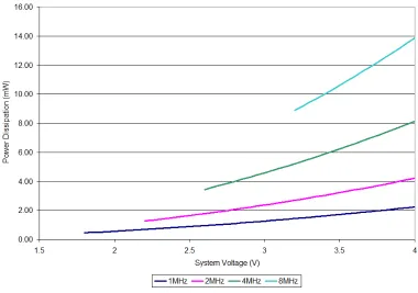
and thenE(t) using the power equation 2.3. These variables are fixed when computing results, but are variables called from a look-up table based upon system configuration, an example of which can be seen in Figure 2.9, showing the effect upon power dissipation as clock frequency is altered.
C∗(d
dtV(t)) + V(t)
RL
−IS = 0 (2.1)
V(t) =IS∗RL+e
− t
RL∗C ∗(V
0−IS∗RL) (2.2)
E(t) =
Z t
0
V(τ)2
RL
dτ (2.3)
E(t) =−1
2∗C∗(2∗IS
2∗R
L2∗ln(e
− t
RL∗C) + (−V
0+IS∗RL)∗ ((−V0+IS∗RL)∗e
2∗t
RL∗C + 3∗I
S∗RL−4RL∗IS∗e
− t
RL∗C +V
0))
Figure 2.9: Mathematical Hardware Model
2.6
Evaluated Scheduling Approaches
In this chapter, offline scheduling refers to finding at design-time one schedule that minimizes expected average energy consumption, while guaranteeing hard deadlines. Online scheduling refers to the computation at run-time, at each occurance of a scheduling point, a new schedule for the remaining tasks such that it minimizes energy consumption while satisfying hard dead-lines. Rebuilding the schedule at each scheduling point allows it to take advantage of the actual execution times of tasks already completed. While having one single schedule obtained offline might be too pessimistic, as information about actual execution times is not used due to the complexity of the problem, the energy and time overhead of computing optimal schedules online is unacceptable. To solve this conflict, we propose to analyze the system and calculate a set of schedules offline and let the decision of which of them to follow be taken at run-time. Thus, the problem addressed in this chapter is that of Quasi-Static Scheduling (QSS) of Rivalrous
2.6.1 Online Scheduling
To demonstrate the benefits of QSS offline scheduling, the simulator was outfitted with four online schedulers capable of satisfying the same design requirements as outlined for the quasi-static offline scheduler. All schedulers are DVS aware and attempt to minimize voltage and therefore MCU frequency over time. All four schedulers are also real-time aware, using the provided worst-case execution times as their sole consideration for picking operating frequencies to guarantee real-time deadlines. All four schedulers operate with a fixed task priority, although have different prioritization strategies. While EDF obtains schedulability, it leaves room open for optimization to reduce energy dissipation by further prioritizing tasks which EDF has given equal priority, as is common in the energy aware literature [60]. First, all tasks are prioritized in accordance with Earliest Deadline First (EDF). Second, SMPS rivalrous tasks are prioritized to run before non-rival tasks of the same priority. Third, tasks that at this point still have the same priority are prioritized in four different schemes consisting of: Shortest Execution Time First, Greatest Execution Time First, Greatest Execution Jitter First, and Shortest Execution Jitter First. The first two online schedulers reorder task priority in order of worst-case execution time, either prioritizing the shortest or greatest. The next two online schedulers reorder task priority in order of execution jitter, or the difference between the task’s worst and best case execution times. Once tasks are prioritized according to policy into a queue, they are executed in accordance with the online DVS/DFS scheduler described in Algorithm 1.
2.6.2 Quasi-Static Scheduler
To demonstrate the effectiveness of our devised techniques compared to the alternatives, a software simulator called the Quasi-Static Scheduler (QSS) was created to satisfy the design rules outlined in section 2.1. This simulator had two overlapping purposes. The primary purpose was to create quasi-static schedules based upon profile data which would allow for the effective clairvoyant scheduling of hard real-time tasks under an event-driven scheduling methodology of a target system with rivalrous hardware. However, to build these schedules and make value judgements between them, the scheduler needed to contain a realistic hardware model and simulator capable of determining the average energy usage of any given schedule.
2.6.3 Schedule Building
Algorithm 1: online Scheduler DVS and DFS Execution Data: Current system state and queue of unexecuted tasks Result: Feasible online Execution
while Tasks remain to execute do
Calculate target frequency by accumulating the worst-case remaining execution cycles / time remaining;
if Voltage is not high enough to finish executing first task given worst-case then Set SMPS to charge to next higher voltage level;
else
Set SMPS target voltage to match target frequency; end
forEvery unexecuted task starting at front of queue do
if Task can run concurrently with already running tasks and SMPS configuration
then
Set task to run immediately; end
end
Execute running tasks until the next switching point occurs; end
the procedure. Starting at this first switching point, the algorithm iterates through all possible system configurations, executes the generated system configuration based upon the mathemat-ical hardware model to calculate the system state of the next switching point, at which point the algorihm will recursively call itself. As the recursive call depth first searches its way into the future, bad schedules which violate correct system state return a failure, allowing the previous switching point to try the next possible system configuration. If they do not fail, and instead complete successfully, the average energy use of the schedule is generated and returned up the recursive call stack to allow higher switching points to compare possible system configurations against each other in terms of expected energy consumption. As this lengthy process completes, winning switching point configurations are finalized and stored.
later, energy use increases to compensate in accordance with the quasi-static schedule. As this design space grows exponentially with each degree of complexity, the amount of time required to complete this design space exploration similarly grows with complexity. An sampling of executions on the intel i5 with four cores at 3GHz utilized to perform the offline schedule building for this project can be seen in Figure 2.11. To minimize this time, the QSS algorithm has been multi-threaded in order to utilize all of the available processing cores.
Algorithm 2: QSS Algorithm for Schedule Building Data: current system state and list of unexecuted tasks
Result: List of switching points and their devised configurations calculate all possible system configurations given Data;
while system configurations remain to be tested do
execute current system configuration to the next switching point; if current configuration reached a valid switching point then
recursively call self to determine all subsequent switching points;
if current configuration has improved utility over previous configurations then store current configuration as winning configuration;
end end
iterate to the next system configuration; end
Figure 2.10: Sample Graphing of All Profiled Executions of Synthetic Task Set
2.7
Scheduler Evaluation
Utilizing the synthetic task set outlined in section 2.7.1, the various online and offline schedulers described in this chapter will be repeatedly simulated in all possible configurations and exe-cutions. The results of these simulations were analyzed to thoroughly compare the simulators against each other as well as verify their respective consistent satisfaction of system state.
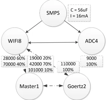
Figure 2.12: Conflict Graph of Simulation Tasks
2.7.1 Synthetic Task Set
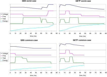
Figure 2.13: Rivalrous, Execution Traces of QSS vs. GETF at 98ms period, or 40% Util.
2.7.2 Quasi-Static Versus Online Scheduling
Worst Case Execution:
Unrun|run Volt SMPS Clock Time Energy e | 1 2 2600mV 2600mV 4MHz 0ms 0.000000mJ master1 6 | 8 2 2600mV 2200mV 2MHz 25ms 0.086865mJ wifi8 4 | 2 1 2205mV 2200mV 2MHz 60ms 0.139912mJ goertz2 4 | 2 1 2200mV 2600mV 2MHz 60ms 0.140529mJ goertz2 0 | 6 2 2600mV 2200mV 2MHz 62ms 0.142742mJ goertz2 adc4 0 | 2 1 2492mV 2600mV 2MHz 71ms 0.158090mJ goertz2 0 | 2 2 2600mV 3200mV 4MHz 71ms 0.158762mJ goertz2 0 | 2 3 3200mV 3200mV 8MHz 73ms 0.168704mJ goertz2 0 | 0 3 3200mV 3200mV 8MHz 83ms 0.255309mJ Finished Execution: 5, 4% 83ms 0.255309mJ U:40%
Most common Execution:
Unrun|run Volt SMPS Clock Time Energy e | 1 2 2600mV 2600mV 4MHz 0ms 0.000000mJ master1 6 | 8 2 2600mV 2200mV 2MHz 10ms 0.036122mJ wifi8 0 | 6 1 2434mV 2200mV 2MHz 24ms 0.059453mJ goertz2 adc4 0 | 2 1 2333mV 2200mV 2MHz 33ms 0.072904mJ goertz2 0 | 2 1 2200mV 2200mV 2MHz 45ms 0.089784mJ goertz2 0 | 0 1 2200mV 2200mV 2MHz 79ms 0.132449mJ Finished Execution: 1, 42% 79ms 0.132449mJ U:26%
Av: 100% 80ms 0.154397mJ -0.025133mJ U:28%
Worst Case Execution:
Unrun|run Volt SMPS Clock Time Energy d | 2 2 2600mV 3200mV 4MHz 0ms 0.000000mJ goertz2 9 | 6 3 3200mV 2600mV 4MHz 2ms 0.009941mJ goertz2 adc4 9 | 2 2 2948mV 3200mV 4MHz 11ms 0.053207mJ goertz2 9 | 2 3 3200mV 3200mV 8MHz 12ms 0.057908mJ goertz2 1 | 8 3 3200mV 2600mV 4MHz 19ms 0.125391mJ wifi8 0 | 1 2 2729mV 2600mV 4MHz 37ms 0.203507mJ master1 0 | 1 2 2600mV 2200mV 2MHz 42ms 0.222753mJ master1 0 | 1 1 2200mV 1800mV 1MHz 78ms 0.276513mJ master1 0 | 0 0 2153mV 1800mV 1MHz 86ms 0.282206mJ Finished Execution: 5, 4% 86ms 0.282206mJ U:40%
Most common Execution:
Unrun|run Volt SMPS Clock Time Energy d | 2 2 2600mV 3200mV 4MHz 0ms 0.000000mJ goertz2 9 | 6 3 3200mV 2600mV 4MHz 2ms 0.009941mJ goertz2 adc4 9 | 2 2 2948mV 3200mV 4MHz 11ms 0.053207mJ goertz2 9 | 2 3 3200mV 3200mV 8MHz 12ms 0.057908mJ goertz2 1 | 8 3 3200mV 2600mV 4MHz 19ms 0.125391mJ wifi8 0 | 1 2 3002mV 2200mV 2MHz 26ms 0.159644mJ master1 0 | 0 2 2719mV 2200mV 2MHz 47ms 0.204830mJ Finished Execution: 1, 42% 47ms 0.204830mJ U:26%
Av: 100% 50ms 0.219299mJ 0.003299mJ U:28%
Figure 2.14: Quasi-Static Scheduler Switching Points Command-Line Output - offline Sched-uler (left) GETF online SchedSched-uler (right) - Graphical version can be seen in Figure 2.13
8MHz speed in order to satisfy the deadlines.
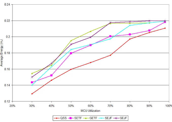
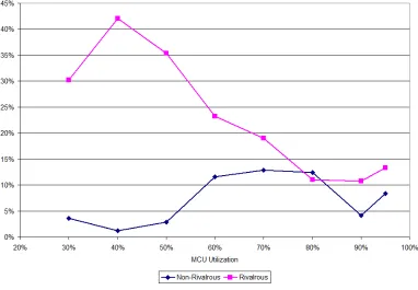
Figure 2.15 shows the quasi-static offline algorithm pitted against the range of online schedul-ing algorithms, and a range of MCU utilizations, as simulated by the QSS application given non-rivalrous tasks. Figure 2.16 consists of the same tasks with their rivalrous nature returned to them. The x-axis represents the worst-case MCU utilization of the given task set at full speed, or 8MHz. The utilization is modified by scaling the hyperperiod of the task set, and therefore the functional deadline for all tasks in the set. Therefore, the respective average MCU utilization is the same for all, at 70% of the worst-case shown on the x-axis. Similarly, the best case is 56% of the worst-case shown on the x-axis.
Figure 2.15: Non-Rivalrous Performance Comparison of QSS vs. a range of online Schedulers
Figure 2.17: Performance Comparison of QSS vs. the best online Scheduler
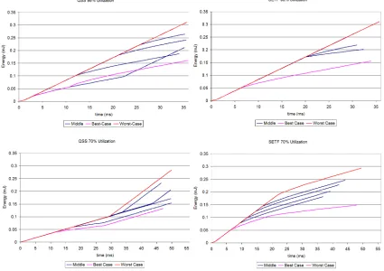
Figure 2.18: Non-Rivalrous Performance Comparison of QSS vs SETF at 98% & 70% Util.
2.7.3 Quasi-Static Scheduler Aided Hardware Design
Figure 2.19: Design Space Exploration of the Power Supply Module for a fixed task set
a large filter capacitor size causes system voltage to drain more slowly and, therefore, operate for longer at high voltages even though such voltages are no longer needed to satisfy deadlines.
2.8
Laboratory Deployment
Figure 2.20: MCU Integrated Power Supply Module
2.8.1 Rivalrous Hardware
The first step in RHS involves hardware abstraction. As can be seen in Figure 2.21, any suffi-ciently complex embedded system will have several lines of scheduling conflict called Rivalrous Resources (RR). Each RR may represent an individual piece of hardware, such as a shared I/O channel, or it may represent an abstract system state, such as noise-free power rails. At the same time, each RR has blocking tasks which block the resource, such as the SMPS applying noise to the power rails, and using tasks dependent upon a resource not being blocked, such as the amplifier which needs noise-free power rails for maximum signal-to-noise operation, as can be seen in Figure 2.22. For RR that represent an individual piece of hardware, such as a UART, tasks tend to be both blocking and using because the hardware is monopolized and cannot be used by another task until this task is done.
2.8.2 Quasi-Static Scheduling
Figure 2.21: Rivalrous Resources
Execution Time (WCET) was taken from Static Timing Analysis (STA) performed by Thrint within the RaPTEX toolchain and combined with profiling information recorded in the lab to produce both a range of possible execution times and a probability associated with each, as can be seen in Figure 2.23. Once this data is collected, it is formated and fed into the QSS simulator.
Figure 2.22: Rivalrous Resources Conflict Diagram
Table 2.1: System Tasks and Rivalrous Resource Conflicts
Tasks 0 1 2 3 4 5 6
0:PS 2 x x x 2 x
1:UWT Read 2 x x x x 3
2:Goertzel x x 1 1 x 1
3:Rx Packet x x 1 1 x 1
4:Network x x 1 1 x 1
5:RC Capture 2 x x x x 3
Figure 2.24: Oscilloscope Trace of System Utilizing RHS and QSS
2.8.3 Laboratory Results
2.9
Conclusions
In this Chapter we introduced the concept of Rivalrous Hardware Scheduling (RHS), which in-volves restricting the execution of rivalrous hardware through software in order to avoid interfer-ence. We demonstrated the useful deployment of RHS techniques in a range of communication designs from projects discussed in later chapters as well as real-world results demonstrating its effectiveness on testing hardware.
Chapter 3
Unified Replay Environment
Embedded systems are driven by the stimuli of the external environment and peripheral de-vices. This tight coupling complicates their development. An embedded application’s compute requirements typically grow over time, possibly outgrowing resources available on the origi-nal processor. This leads to the need to predict the application’s performance on a different processor or even a different instruction set architecture.
Determining the system’s performance on the new platform requires porting platform-specific code. Because this is a slow and tedious process, onlykernels, which represent what the programmer believes to be critical program sections, are ported and evaluated. These kernels are inaccurate due to their incomplete nature. The kernels may not be sufficiently representa-tive of the application. Program memory requirements are merely estimates unless the code is ported to the point of compilation. Energy consumption estimates depend upon the run-time of the actual code, which can only be estimated in this way. Not only do microkernels not ac-curately represent the entire application, they do not factor in I/O-bound portions (e.g. ADC conversion delays, communications with LCD controller, flash, and UART). How much time is spent in these activities is typically unknown without taking the time to profile an application, but embedded software development toolchains typically lack profiling support. This chapter describes tools, primarily a hardware abstraction layer, to solve these problems by simplifying the porting of a entire application across multiple processor platforms and architectures to allow accurate performance prediction.
16-bit MCU’s. We characterize processor utilization and memory requirements.
3.1
Related Work
3.1.1 Input Recording and Replay
There is extensive work on recording inputs and events to enable replay of a program’s execution. Most of this work seeks to simplify debugging, as in some systems it is tedious, difficult, or even impossible to reproduce exactly the sequence of events leading to the triggering of the bug. Efficient cyclic debugging requires the ability to replicate the program’s execution exactly and repeatedly.
Cornelis et al. provide a survey of the issues involved and various solution approaches [9]; we follow their explanation here. Desirable features of any approach include accuracy, non-intrusiveness, and time- and space-efficiency. A replay approach based on sequential (re-)execution of a program must deal with three sources of non-determinism: input instructions, interrupts, and memory modified by other devices.
• Input instructions read information from the external environment and peripheral devices. Computer systems with protected operating modes typically prevent a user program from directly executing these instructions and instead encapsulate them insystem calls.
• Interrupts may operate asynchronously and independently of the main program’s execu-tion, and may change the contents of data memory.
• Memory may be explicitly modified by peripherals such as direct memory access con-trollers or other processors in a multi-processor system. In the case of memory-mapped I/O, it also may change in response to the external environment and peripheral devices.
Some of the basic features of input record and replay are present in commercial simulators for embedded processors. For example, AVR Studio [2] is an integrated development environment for Atmel AVR microcontrollers. It allows debugging via a simulator or on a physical in-system MCU. When operating in the simulator mode, it is capable of recording output port values with time stamps in a log file. The simulator also allows the use of a stimulus file to specify input port values over time. Although the log and stimulus file have the same format, they cannot be used for record/replay. What is needed is a way to create a stimulus file automatically from the input port values while the program executes on a remote processor in a real system.
There are many examples of record/replay tools which target personal computers or work-stations rather than embedded systems.
targets Java applications and instead focuses on multithreaded programs while not supporting I/O operations beyond some windowing and network events.
Tornado [8] tracks and recreates a Linux system’s writes from kernel to user space. Certain system calls (e.g. read()) only affect an easily determined area of user memory. Instrumenta-tion of more difficult funcInstrumenta-tions (e.g. ioctl()) depends upon the fact that the kernel is limited to using a set of primitives to write to user memory. In Tornado, these primitives are modified to keep track of the addresses written.
Recorded program execution information can also be used to allow reverse playback of a program, simplifying debugging. Examples of such tools include Recap [40], Spyder [1] and Simics Hindsight [58].
Attributes of some systems further complicate debugging and record/replay support. In real-time systems, program correctness depends upon execution real-times. Hence any overhead from record/replay support should be minimal and predictable. Distributed systems have multiple processors but do not have global state information or global time, complicating the creation of a coherent view of events and when they occurred. Dodd and others developed methods to handle record and replay debugging and monitoring of distributed real-time systems [13, 56].
Replay debugging has been developed further to simplify cyclic debugging of non-deterministic parallel programs by providing repeatable thread switching. Other work deals with shared mem-ory accesses to help with the debugging of multithreaded code and multiprocessors. This work includes Instant Replay [34], RecPlay[49], and Reversible[6]. Still other work models such sys-tems with asynchronous concurrency [20]. These techniques address issues which are beyond the scope of our work.
Implementation options include software and hardware. Software solutions require the sys-tem’s processor to execute code to record or replay inputs, while hardware approaches reduce or eliminate this loading. A software-only solution provides great flexibility and portability at the expense of greater interference in the execution of the system being monitored. In addition, the program may need to be modified, potentially leading to the insertion of additional bugs.
Adding dedicated hardware (e.g. a logic analyzer or in-circuit emulator (ICE)) to record and reproduce inputs [57] eliminates delays in the program’s execution. This can be critical for time systems, as execution time affects program correctness. Systems with looser real-time requirements (or none at all) may be able to tolerate the timing overhead and variations introduced by a software approach.
Our approach is unique in the following ways:
• Our approach supports the recording and replay of input instructions, unlike the 11 execution replay systems surveyed by Cornelis [9].
• Our approach supports the recording and replay of all interrupts. Of the 11 systems examined by Cornelis [9], only three support interrupts, and those only support those used for scheduling.
• We classify events (input instructions or interrupts) as dependent or independent of pro-gram execution. This allows our approach to support different processor clock speeds, which is needed for cross-platform and other analysis. This is described in greater detail in Section 3.2.3.
• We target embedded systems with tight timing requirements and evaluate the timing fidelity of our approach.
Due to the characteristics of the embedded systems we target, our approach does not attempt to solve some of the problems tackled by other researchers. We do not attempt to support system calls, as the targeted processors do not offer protected modes. Nor do we address multiprocessor systems or shared memory. Our approach requires recompilation of the application, but this is reasonable given the nature of porting.
3.1.2 Embedded Benchmarks
Performance evaluation benchmark suites for embedded systems fall into two categories. First, there are various benchmark suites which have been developed to represent embedded pro-cessing1. Second, there are microkernels which microcontroller vendors use for marketing2.
As these microkernels are small and not sufficiently comprehensive, we do not consider them further here.
The EDN Embedded Microprocessor Benchmark Consortium (EEMBC) provides various benchmark suites to cover different segments of the marketplace: Consumer, Digital Entertain-ment, Java, Networking, Telecom, Office Automation and Automotive [59]. Each benchmark suite is composed of kernels chosen to represent the application domain. For example, the Au-tomotive suite contains functions performing FIR and IIR filtering, time-to-frequency domain conversions (and vice versa), bit manipulation, floating point emulation, matrix math, embed-ded networking, pointer chasing and automotive-specific functions for sensing vehicle state and control.
1These are an alternative to SPEC, which is not appropriate for this domain [16]. 2
MiBench consists of freely-available C code for embedded systems [25]. It targets embedded systems with large amounts of memory and fast CPUs. Sample applications are grouped as in EEMBC: automotive and industrial control, networkings, security, multimedia consumer devices, office automation and telecommunication.
MediaBench and MediaBench II focus on media processing code written in C [35, 18]. Ar-eas include video codecs, image codecs, audio codecs, speech (compression and recognition), security (encryption, decryption and hashing), graphics (rendering, lighting and shading), com-munication (including error control coding), and media analysis (segmentation and feature extraction).
Using these benchmarks suites to predict an application’s performance across multiple low-end embedded processors has several limitations:
• No benchmark set measures thedeveloper’s actual application. Instead, what is suspected to be the most representative benchmark is used. However, without profiling the appli-cation one cannot verify that suspicion.
• These benchmarks rely upon file system support from the operating system. Most low-end embedded systems lack such a file system, making porting the benchmarks non-trivial.
• In order to enable portability across processors, I/O operations and ISRs are deleted. In this work we seek to retain these aspects of the program, allowing more accurate performance analysis.
• Memory requirements are not representative of programs for low-end MCUs, which often have RAM sizes measured in kilobytes or tens of kilobytes. For example, only 12 of the 38 benchmarks in MiBench have a data segment smaller than 50 kilobytes. Porting the benchmarks to fit within the limited RAM is non-trivial.
In this paper we contribute a method and tools to allow a system designer to evaluate the performance of his or her own application on the target processor without having to resort to the proxy of a benchmark (assuming it can even be ported to the target processor).
3.2
Methods
We useinput virtualization to record or replay inputs to the system, enabling the deterministic duplication of a program run. Hence URE provides an hardware abstraction layer. Figure 3.1 depicts the entire process of environment record and replay.
Figure 3.1: Overview of RE approach
is then used to generate a C source file (rec data.c) declaring a data structure initialized with the recorded data. The program is recompiled for the target architecture, including rec data.c to provide inputs for the replay mode.
In thereplay mode, the program takes inputs not from the original environment, but instead from the locally stored data. This allows reconstruction of input operations or interrupts at the correct times. Input virtualization is implemented by making use of macros, described below.
3.2.1 Language Selection
The C language was chosen for URE. C is the dominant language for embedded systems due to its flexibility, efficiency, and higher abstraction level than assembly language. C offers much better portability than assembly language, simplifying analysis across architectures.
3.2.2 Event Description Storage
Data describing events are stored in an array holding linked lists of event descriptors (ULLA, Unified Linked List Array). Each virtualized device has a list within ULLA. Each list consists of descriptors, each of which describes the input data, the absolute time or time delay, and a pointer to the next node in the list.
3.2.3 Event Classification
Events are classified to provide realistic system behavior as parameters which affect changes in the speed of program execution. For example, increasing the processor clock frequency will not affect time delays of serial communication. Factors affecting program speed include the compiler, optimization settings, processor clock speed and processor ISA.
RE supports two types of events: Independent andDependant. Independent (asynchronous) events occur at a fixed point in time regardless of program state or progress. For example, a temperature sensor’s value may change at a certain time regardless of program activity. Changing the speed of the processor will not affect when this value changes. Such events are described with an absolute time stamp. Dependent events are associated with a specific program location or state. For example, when transmitting serial data with a UART, the Transmit Complete interrupt will happen some time after the data is loaded into the UART. Increasing the processor clock speed may cause the data to be loaded into the UART earlier, leading to an earlier Transmit Complete interrupt. These events are described with a time delay relative to the triggering event. Dependent events can either be immediate or delayed, whether the delay is zero or not.
We assume that the delay of a dependent delayed event is constant regardless of processor clock speed, compiler, optimizations and ISA. For most peripherals this is correct, but there are some exceptions (e.g. onboard analog to digital converter). For these exceptions, the time differences across ISAs are minor compared with the computation time.
We have developed a tool called TDM (Time Data Modifier) which adjusts timing informa-tion in the event log (rec data.c) to correctly represent event timing on target processors with clock rates different than the host processor. TDM adjusts the times for both independent and dependent events.
It would be possible to extend TDM to allow time stamp adjustment to reflect changes to the environment or peripherals (e.g. slower ADC, faster serial communications). We leave this as future work.
We rely upon the programmer to classify events manually. However, it would be possible to automate portions of this task by categorizing operations based upon the peripheral which is being accessed or the type of interrupt.
3.2.4 Time Subsystem