Development of Digital Signal Processing and Statistical Classification Methods for Distinguishing Nasal Consonants

Abstract

WANG, MENG. Development of Digital Signal Processing and Statistical Classification Methods for Distinguishing Nasal Consonants. (Under the direction of David McAllister.)

For almost half a century, people have been looking for efficient classifiers to distinguish two nasal sounds, /m/ from /n/, uttered by a single speaker. From the middle of the last decade, there has been little progress in research on this topic. In recent years, we, researchers of the Voice I/O Group in Department of Computer Science at North Carolina State University, have conducted some new trials on this classical problem. In this thesis, those trials are briefly summarized. Instead of simply using the Fourier transform to produce the spectra as people usually did in the past, the author uses other kinds of transforms to

extract more feature differences between /m/ and /n/. The new transforms can be the alternatives of frequencies, such as singular values or eigenvalues, or even other transforms

such as wavelets, which can deal with non-stationary systems quite well. We combine

together the old and new features to get a larger feature vector, which will bring more

classification information. We collect multiple voice samples of a single speaker and

calculate the above feature representations, then use them as input of some popular statistical

classification techniques, such as Principle Component Analysis (PCA), Discriminant

Analysis (DA), and Support Vector Machine (SVM). By way of one training process, one

Development of

Digital Signal Processing and Statistical Classification Methods

for Distinguishing Nasal Consonants

By

Meng Wang

A thesis submitted to the Graduate Faculty of

North Carolina State University

in partial fulfillment of the

requirement for the Degree of

Master of Science

Operations Research

Raleigh

2003

APPROVED BY:

_____________________________________ __________________________________

PERSONAL BIOGRAPHY

Meng Wang was born on February 26, 1975 in Suxian City, P.R.China.

He started school when he was six. In the same city, he continued his education

until he graduated from high school in 1992.

Meng then went to Nanjing City in Jiangsu Province to attend college in

Southeast University. And in May 1996, he graduated with honors, receiving a

Bachelor of Science degree in Mathematics, with a concentration in Applied

Mathematics. He was also approved to be a candidate of a Master of Science in

the same department without taking any entry tests.

He continued academic study in Southeast University and graduated with

the Master degree in May 1999. Then he came to the United States to enter a

Ph.D program in Operations Research Program. From February 2001, he began

to work with the Voice I/O Group on the Lip Sync Project. From September

2001, he started working on nasal identification problem.

In March 2003, Meng stopped his Ph.D study and transfered to a thesis

Master student. He is scheduled to graduate in August 2003.

Meng’s main interests include web searching, reading and anything

related to computer software. He also has interest on driving and sports, such as

TABLE OF CONTENTS

LIST OF TABLES………. iv

LIST OF FIGURES……… v

LIST OF NOTATIONS AND SYMBOLS……….viii

Chapter 1 Introduction and Background………. 1

1.1 Speed Production……….. 2

1.2 Articulatory Phonetics for Nasals……….… 5

1.3 Acoustical Properties of Nasals……… 7

Chapter 2 Recent Progress on Identifying /m/ and /n/……….. 15

2.1 Moment Space Methods………..……… 15

2.2 The Combined Spectra Method………... 18

2.3 Other Progress………..……… 18

Chapter 3 The Combined Spectra Method……….… 19

3.1 Review of Ideas………... 19

3.2 Algorithm, Result and Discussions………... ..26

Chapter 4 Feature Extraction Using Singular Value and Eigenvalue Tests…….. 33

4.1 Singular Value Tests……….. 33

4.2 Eigenvalue Tests………. …53

4.3 Conclusions………. 61

Chapter 5 Statistical Classification Techniques………. 62

5.1 Bayes Rule and Discriminant Functions……… 62

5.2 Adding More Independent Components into the Feature Parameter Set ……….. 65

5.3 Dimensionality Reduction and Number of Training Samples…….. 68

5.4 PCA with 52 Parameters………..……... .. 73

5.5 Discriminant Analysis……… 73

5.6 Support Vector Machine……… 78

5.7 Experimental Results……… 82

Chapter 6 Conclusions and Future Study……….. 90

List of References……….… 92

LIST OF TABLES

Page

1.1

Place of Articulation……… 10

5.1 Locations for Anti-formant/Formant of Nasals……….. .73

5.2 Data for Syllable-initial Case for Two Speakers Used in DA and

SVM……….82

5.3 Data for Syllable-final Case for Two Speakers Used in DA and SVM

………83

5.4 Data for Syllable-initial Case for Two Speakers Used in PCA Method

………84

5.5 Data for Syllable-final Case for Two Speakers Used in PCA Method

………84

5.6 Performance of PCA in Syllable-initial Case………..84

LIST OF FIGURES

1.1

Schematic View Of the Human Speech Production Mechanism………. 3

1.2

Block Diagram of Human Speech Production………. 4

1.3

Spectrum of the Vowel “ah” Showing Three Formant Regions……….. 8

3.1 Release Point, the Nasal-boundary and Vowel-boundary Windows…. 21

3.2 Bark Scale VS Frequency in Hertz……… 24

3.3 A Spectrum of Length 128 under a Sampling Rate of 22050 Hz……...25

3.4 The 22 Bark-Scale Representation of the Above Spectrum……….… 25

3.5 Syllable-initial Case………. 30

3.6 Syllable-final Case………... 31

4.1 Release Point and the Five Glottal Pulses……… 35

4.2 The Color and Amplitude………. 38

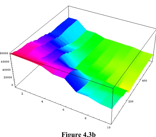
4.3a Waveform of /im/..………. 39

4.3b The First 10 Singular Values Generated by the 3 Glottal Pulses in the

Middle of the Signal …..………..……….. 39

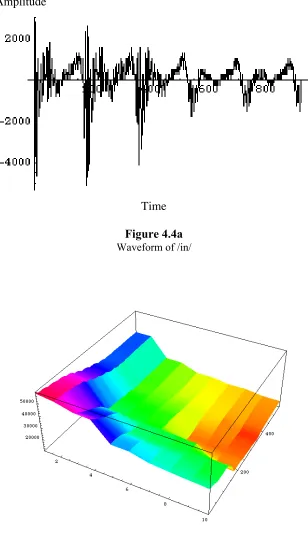
4.4a Waveform of /in/…..………... 40

4.4b The First 10 Singular Values Generated by the 3 Glottal Pulses in the

Middle of the Signal……… 40

4.5a Waveform of /mi/……… 41

4.6a Waveform of /ni/……… 42

4.6b The First 10 Singular Values Generated by the 3 Glottal Pulses in the

Middle of the Signal……… 42

4.7 Seven Glottal Pulses for a Pure /

/ Sound in Time Domain……….. 44

4.8 Plot of the Stable Singular Values along the 7 Glottal Pulses When the

Size of the Matrix is Equal to the Period of the Glottal Pulse………. 45

4.9

Plot of the Unstable Singular Values along the Same 7 Glottal Pulses

When the Size of the Matrix is Equal to 1.2 Times the Period of the

Glottal Pulse………. 45

4.10

Plot of the Unstable Singular Values along the Same 7 Glottal Pulses

When the Size of the Matrix is Half of the Period of the Glottal Pulse

………...46

4.11a Singular Value Track for /ahm/ ……….49

4.11b Singular Value Track for /ahn/ ……….49

4.12a Singular Value Track for /eem/ ……….49

4.12b Singular Value Track for /een/ ………. 49

4.13a Singular Value Track for /ehm/ ……….49

4.13b Singular Value Track for /ehn/ ………. 49

4.14a Singular Value Track for /oom/ ……….50

4.14b Singular Value Track for /oon/ ………. 50

4.15a Singular Value Track for /moo/ ……….50

4.15b Singular Value Track for /noo/ ………. 50

4.16b Singular Value Track for /nee/ ………. 51

4.17a Singular Value Track for /meh/ ……….51

4.17b Singular Value Track for /neh/ ………. 51

4.18 Left and Right Windows ……… 56

4.19a Waveform of /am/ ………. 58

4.19b The Spike Generated by EVD IV….………. 59

4.20a Waveform of /an/ ……….. 59

4.20b The Spike Generated by EVD IV….………. 59

4.21a Waveform of /ma/ ………. 59

4.21b The Spike Generated by EVD IV….………. 60

4.22a Waveform of /na/ ………. 60

4.22b The Spike Generated by EVD IV….………. 60

5.1 Performance of LDA in Syllable-initial Case on Speaker DB……….. 86

5.2 Performance of LDA in Syllable-initial Case on Speaker DW………. 86

5.3 Performance of LDA in Syllable-final Case on Speaker DB………… 87

5.4 Performance of LDA in Syllable-final Case on Speaker DW………... 87

5.5 Performance of SVM in Syllable-initial Case on Speaker DB………. 88

5.6 Performance of SVM in Syllable-initial Case on Speaker DW……… 88

5.7 Performance of SVM in Syllable-final Case on Speaker DB…………89

LIST OF NOTATIONS AND SYMBOLS

Notations

Tables, figures and equations in each chapter are numbered

serially. The first number indicates the chapter number, and the

second number indicates the table, figure or equation number. The

two numbers are separated by a dot. If a reference is made to, say

equation number (3.2) in a chapter, it means equation 2 of chapter 3.

Vectors are in general column vectors under lower-case; matrices are

under capital-case.

---Symbol Definition

Symbols are listed using alphabetical order for lower case,

upper case, Arabic and Greek formats. The page numbers where the

symbols are used for the first time are also indicated.

[1]

: scale-factor 23

[2]

: second central moment 16

[3]

26

[4]

,

_:

_{dimension of feature vectors}

₆₉

[5]

: exponential function 64

[6]

: mean vector 27

[7]

: f

requency in Hertz

16

[8]

: standard deviation 27

[11]

: first moment 16

[12]

: probability density function 16

[13]

,

: feature vectors 57

[14]

,

:

PCA-derived vector

57

[15]

: Mahalanobis distance 29

[16]

: Mahalanobis distance 77

[17]

:

feature vector

26

[18]

[19]

,

:

LDA - transformed training data 77

[20]

: transformation matrix 77

[21]

: Traunmüller's approximation for bark scale 24

[22]

,

,

,

: covariance matrix 28

[23]

: covariance matrix 70

[24]

_{: transpose of}

₂₆

[25]

: d

eterminant of

64

[26]

: speed of sound 11

[27]

: expectation values 26

[28] FFT: Fast Fourier Transform 27

[29]

: Sampling rate 15

[30]

:

the Generalized Approximate Cross Validation 79

[31]

: the Generalized Comparative Kullback-Liebler distance 80

[32]

: glottal pulse 15

[33]

: The Reproducing kernel Hilbert space (RKHS) 80

[34]

: Transfer function 7

[36]

:

R

eproducing kernel 80

[37]

: total length of the vocal tract 11

[38]

: mass: 16

[39] N1, N2, N3: nasal formants 11

[40]

,

:

numbers

28

[41]

: o

utput signal

23

[42]

: probability 62

[43]

: Pitch 15

[44]

: spectrum 16

[45]

,

: covariance matrix 75

[46]

: transformation matrix 75

[47]

_,

_{: transformation matrix 57}

[48]

-transform of the input signal:

7

[49]

-transform of the output signal:

7

[50]

: eigenvectors 26

[51]

,

: training data feature vector 27

[52]

: PCA-derived vector 28

[53]

,

: testing data feature vector 27

[54]

: PCA-derived vector 28

[55]

:

PCA-derived vector 26

[56]

,

: m

eans

55

[57]

: m

ean

75

[58]

:

Discriminant function

64

Chapter 1

Introduction and Background

Distinguishing between two nasal consonants, /m/ and /n/, has been a classical problem

of acoustic phonetics for half a century. The progress of this topic was well summarized in [1]. Nearly all the work in this area suggests that the information needed to solve this problem lies in the shape of the various spectra of the nasal consonants themselves as well as the surrounding sounds, including the transitions to and from the nasals. Phoneticians for years have extracted some useful information, such as the different locations of the anti-formants and the anti-formants between /m/ and /n/, from the spectrum. These differences are reflected in the shape of the various spectra. In addition, the phoneticians have observed that the starting frequency of the second formant provides a cue for distinguishing /m/ from /n/, again a matter of spectral shape. In 1994, Harrington proposed the Combined Spectra Method [1], which uses the spectral information from both the nasal sounds and the vowel sounds around the nasals. The Combined Spectra Method shows the best performance on identifying /m/ and /n/ until recent years, although the accuracy is no more than 94% for both syllable-initial (nasals precede the vowels) and syllable-final (nasals succeed the vowels) cases. To better understand this important method, we duplicate and discuss it briefly in Chapter 3. However, in Harrington’s experiments, the data were collected for multiple speakers. In this thesis, we are conducting experiments for one single speaker.

acoustically very similar while corresponding to vastly different visemes. More specifically, the lips are closed for /m/, and open for /n/.

The remainder of this thesis is organized as follows. Chapter 1 provides the background

of this study, which contains a brief description of the phonetic and acoustical properties of

nasals. Chapter 2 presents an overview of past efforts on this topic. Chapter 3 duplicates the

Combined Spectra Method and re-evaluates its performance. Chapter 4 sheds light on some

new approaches, such as eigenvalue tests and singular-value tests, that are used to produce

more feature vector components. Chapter 5 uses some efficient statistical classification

methods to process the features derived from the Combined Spectra Method, singular-value

or eigenvalue test, moment-space method, root-mean-square values, and the locations of

anti-formants and anti-formants. Chapter 6 gives the conclusions and topics of future research.

1.1 Speech Production

Overview

Normal speech sounds are produced by modulating an outward flow of air. For most sounds, the lungs furnish the stream of air, which flows between the vocal folds (cords), and causes them to vibrate, thereby modulating the air. The air then passes through several vocal cavities before it exits from the body through the mouth and to a slight degree through the nostrils. Speech sounds produced in this way are called voiced sounds.

Figure 1.1

Schematic View of the Human Speech Production Mechanism, from which one can see the air going through Pharyngeal, Oral, and sometimes Nasal cavities, after being modulated by the vocal cords.

Those three cavities act as three filters to produce different kinds of voiced sounds.

Figure 1.2

Block Diagram of Human Speech Production.

In the production of the vocal sounds, the vocal folds are drawn closely together by

muscles, the air in the lungs is exhaled, the pressure below the vocal folds rises, and the

closed folds are forced apart. The resulting rapid upward flow of air causes a decrease in

pressure between the folds due to the Bernoulli Effect (explained later). The decrease in

pressure, along with the elastic forces in the tissues, causes the folds to move together,

partially blocking the passage and thus reducing the air velocity. The reduced air velocity

increases the pressure below the folds and causes the process to repeat again. The sound

produced in this manner is called a glottal sound.

The fundamental frequency of the resulting complex vibration depends on the mass and

tension of the vocal folds. Men have longer and heavier vocal folds than women, with a

typical fundamental frequency of about 125Hz; women are about one octave (a factor of two)

The glottal sound passes through several vocal cavities - the Pharyngeal (throat), oral,

and nasal cavities, as mentioned above - that further change the sound of the wave emitted.

The shape of the throat and nasal cavities is fixed for each individual and to a large extent

determines the sound of the voice. They cannot be changed much voluntarily unless the

speaker holds his nose and talks. The oral cavity changes shape through the movement of the

tongue, lower jaw, soft palate, and cheeks to determine specific voiced sounds. The variation

in shape of the nasal cavity for each speaker brings certain difficulties for the design of a

speaker-independent algorithm.

It is necessary here to explain the meaning of Bernoulli’s Principle in more detail. In a

fluid flow situation, such as in water or air, the pressure in the moving fluid is lower at places

where the speed of flow is greater. In the case of air rushing through the vocal folds, there is

a lower-pressure area in the restricted region between the folds, leading to a Bernoulli force.

This force and tension in the vocal folds causes the folds to close. Immediately after the

vocal folds close, the air pressure builds up in the trachea, rapidly forcing the folds open once

again. The burst of air through the vocal folds again creates the Bernoulli force, and the cycle

is repeated. The rate of opening and closing determines the frequency of the resulting vocal

sounds.

The frequency of vibration of the vocal folds is determined primarily by the controlled

tension in the vocal folds, whereas the amplitude of the vibration is affected by increasing or

decreasing the rate of the air flow between the folds.

1.2 Articulatory Phonetics for Nasals

Consonants and Vowels

oral cavity by moving the articulators and changing the place of articulation in the oral cavity.

Nasal Speech Production

The symbols /m/ and /n/ represent the two consonants we discussed in this paper. Together with /h/ as in “thing”, they are called nasals. When people produce /m/ or /n/, air

escapes not only through the mouth (when people open the lips), but also through the nose (nasal cavity). From Figure 1.1, the roof of the mouth is divided into the hard palate and the soft palate (Velum). Hanging down from the end of the velum is the uvula. When the velum is raised all the way and touches the back of the throat, the passage through the nose is cut off and air can only escape through the mouth (oral cavity). Sounds produced in this way are called oral sounds. For example, /b/ as in “bed” is an oral sound. When the velum is

lowered, air escapes through the nose as well as the mouth. Sounds produced in this way are called nasal sounds. The consonants /m/, /n/ and /h/ are the only nasal sounds in English.

All other consonant sounds are oral.

Common Properties of /

/ and /

/

Phonetically, /m/ and /n/ have many similarities that cause difficulties when

identifying them from each other. Nevertheless, they also have some phonetic differences when considering other classification criteria, such as place of articulation. /m/, together with /p/ and /b/, are called bilabials, since they are articulated by bringing both lips

together. /n/ belongs to the alveolar class because it is articulated by raising the front part of the tongue to the Alveolar ridge. If speakers pronounce the word “new” (/nu/), they can feel the tongue in close proximity to the bony tooth ridge as /n/ is pronounced. The mouth is not closed and lips are open.

1.3 Acoustical Properties of Nasals

Acoustic characteristics of nasal consonants and nasalized vowels are perhaps the least well understood of all classes of speech sounds. One way to model nasal consonants is to assume that there are three tubes, or filters, one for each of the nasal, oral, and pharyngeal cavities. These filters modify the input signal generated from the vocal chords.

Before further discussion on this topic, some terminology is introduced.

1. Zeros and Poles of Filters

In the case of nasal sounds, the locations of zeros correspond to the frequencies of the

anti-formants, and the locations of poles correspond to those of the formants [25]. We define

zeros and poles before discussing anti-formants and formants. We assume the reader is

familiar with linear time-invariant filters [30].

The transfer function of a linear time-invariant discrete-time filter is defined as

) (

) ( ) (

z X

z Y z

H = (1.1)

where X(z) denotes the z-transform of the input signal, and Y(z) denotes the z-transform

If there exists one complex number z so thatY(z)=0, we call z a zero. Similarly, if

there exists a z so thatX(z)=0, we call z a pole.

The locations of zeros and poles provide useful insights into the performance of a filter. The locations are also important information when designing a digital filter.

For more details on zeros, poles, transfer functions, and other backgrounds of digital signal processing, refer to [28] and [30].

2. Formants

When examining a spectrum of a periodic signal waveform, we can see falls and rises in the spectral shape that span a wide frequency range (The unit is Hz in the case of human speech). These peaks, called formants, are estimates of the resonance of the vocal tracts. See Figure 1.3 for formants.

Figure 1.3

Spectrum of the Vowel "ah" Showing Three Formant Regions. The vertical lines

represent harmonics produced by vibration of the vocal cords and based on fundamental frequencies. These harmonics are resonated by the vocal tract to create the

vowel's characteristic spectral shape.

of this filter is approximately constant [25]. This means that if there is a change to the source but a minimal change to the filter, the formant center frequencies do not change and there is a minimal change in the long-term spectral trend of the combined sound output.

3. Anti-formant

The filter spectrum for nasal sounds is characterized by both formants and anti-formants. Anti-formants are the dips in the filter spectrum. They are introduced whenever there is more than one acoustic path from the source to the mouth opening. When producing nasal sounds, two acoustic paths are formed, from the glottis into the nasal cavity and from the glottis into the oral cavity.

4. Place of Articulation

Place of articulation is the relationship between the active and passive articulators

(where to articulate, such as lips or tongue) as they shape or impede the air-stream. The

active articulator usually moves in order to make the constriction. The passive articulator

usually remains static and is approached by the active ones.

The International Phonetic Alphabet recognizes the following places of articulation in

Table 1.1 Place of Articulation

Bilabial The point of maximum constriction is made by the coming together of the two lips.

Labiodental The lower lip articulates with the upper teeth.

Dental The tip of the tongue articulates with the back or bottom of the top teeth.

Alveolar The tip or the blade of the tongue articulates with the forward partof the alveolar ridge. A sound made with the tip of the tongue here is an apico-alveolar sound; one made with the blade, a lamino-alveolar.

Postalveolar The tip or the blade of the tongue articulates with the back area of the alveolar ridge.

Palatal The front of the tongue articulates with the domed part of the hard palate.

Velar The back of the tongue articulates with the soft palate.

Uvular The back of the tongue articulates with the very back of the soft palate, including the uvula.

Pharyngeal

The pharynx is constricted by the faucal pillars moving together (lateral compression) and, possibly, by the larynx being raised. "It is largely a sphincteric semi-closure of the oro-pharynx, and it can be learned by tickling the back of the throat, provoking retching"

Glottal The vocal folds are brought together; in some cases, the function ofthe vocal folds can be part of articulation as well as phonation, as in the case of [h] in many languages.

Please see [4] for more detail.

Next, we consider the acoustical properties of nasals.

Zero vs Anti-formant / Pole vs Formant

Let H(z) be the transfer function of the filter that creates the output sound from the

input.

In the case of nasalized vowels, the mouth provides the main path and the nasal cavity is the shunt. Since the shape of the nasal cavity is fixed, the location of this zero is constant (typically at about 1500Hz). Hence instead of a movable zero being added to (and perturbing) a constant set of poles, there now is a fixed zero added to (and perturbing) the variable poles of the vocal tract [25].

From theoretical considerations of vocal tract modeling, it can be shown that the average spacing between formants is C_sound /(2L)Hz, where C_sound is the speed of sound,

ond centimeter

C_sound =34000 /sec , and L is the total length of the vocal tract.

When producing nasal sounds, the formants depend on the combined nasal-pharyneal tract (with a length of about 20cm for an adult male), while a major anti-formant is introduced by the side-branching oral cavity (with a length of about 17cm for an adult male). Then, the spacing between the nasal formants is C_sound /(2L)=

34000/40=850Hz. If the sampling rate is F_s =22050Hz, the Nyquist limit of frequency is

22050/2=11025Hz. Hence, there exist 11025/850=13 formants in the 0-11025Hz range.

The single major anti-formant frequency depends on the length of the side-branching oral cavity, so its value could be varied for different kinds of places of articulation.

The above discussion shows that for a sampling rate of 22050Hz, the transfer function H(z) should have 13 fixed poles and one single zero with a variable location

when producing nasal sounds.

For more information on the relationship between zeros and anti-formants, and between poles and formants, please refer to Section 7.3 and 7.4 of [25].

The spectra of nasal consonants are characterized by nasal formants (labeled N1, N2, N3, …) which are due to the combined nasal-pharyngeal tube. For nasal and pharyngeal tubes with lengths typical of those of an adult male vocal tract, the first nasal formant, N1, is calculated to occur in the 300 to 400 Hz region; higher nasal formants occur approximately at 800Hz intervals [22][25].

In uvular and post-velar articulations, the oral cavity is effectively cut off from the nasal-pharyngeal tube and therefore has little effect on the resulting spectrum. For nasals produced with the tongue at the far back of the mouth, the spectrum is determined almost entirely by nasal formants. However, when the tongue articulation is further forward in the mouth, as in the production of palatal, alveolar, or bilabial nasals, the oral cavity acts as a side-branching resonator to the main nasal-pharyngeal tube and introduces oral anti-formants into the spectrum. The first anti-formant frequency occurs at a quarter-wavelength of the oral cavity, that is, at C_sound/(4l_m) Hz, where l_m is the length of the

side-branching oral cavity with a unit of centimeter, and C_sound is the speed of the sound.

This implies that the frequency of the first anti-formant varies inversely with the length of the oral cavity, being lower for /m/ and higher for /n/.

In general, the effect of introducing oral anti-formants is to “flatten” the spectrum, particularly if nasal resonances and oral anti-formants coincide, and to lower its amplitude. In spectrograms, nasal consonants typically show overall amplitude dips and nasal formants that are very low in amplitude.

Moreover, oral formants occur in the spectrum when nasal consonants are produced. However, since these are likely to be close to the oral anti-formants in frequency, they are usually very low in amplitude [25].

Other Acoustic Characteristics of Nasal Consonants

1. Nasal formants occur at approximately 700-800Hz intervals, beginning with N1 that

locates around 250-300 Hz.

2. Nasal formant bandwidths are broader than those of oral vowels.

3. The first nasal formant has very high amplitude compared with that of higher formants.

4. Anti-formant exists in the 500-1000Hz range for /m/ and in the 1000-2000 Hz range for /n/.

The last characteristic shows that the anti-formant regions of /m/ and /n/ are not overlapping. In fact, there are also some similar non-overlapping observations for the formant regions. It is agreed that the first three formants for /m/ and /n/ are 250, 1000, 2000Hz and 250, 2000, 2700Hz, respectively. So, theoretically, the spectrum should show a clear distinction on amplitude around 1000Hz between /m/ and /n/ cases. However, we cannot directly use the locations of formants and ant-formants to identify /m/ and /n/ for the following reasons:

1. _{They represent a set of harmonics with high energy, not just a single clearly}

identifiable harmonic, and within the band there is variation in terms of which harmonics, and with what energy, they contribute to the formant.

2. The shape of the formant/anti-formant is often variable over the course of a few dozen milliseconds.

3. The starting and ending points are co-articulation dependent. 4. There is a considerable amount of intra-speaker variation.

Place of Articulation and Nasal-Vowel Transition Boundary

acoustic analysis of natural speech data, have suggested that the waveform of the nasal-vowel transition boundary is where the crucial information is contained.

More About Nasalization of Vowels

In the end, it is necessary to mention the concept of nasalization of vowels since in this thesis we will mainly focus on the transition regions between vowels and nasals. Nasalization of vowels is unavoidable during the production of those transition regions.

Vowels, like consonants, can be produced either with a raised velum that prevents the air from escaping through the nose, or with a lowered velum that permits air to pass through the nasal passage. When the nasal passage is blocked, oral vowels are produced; when the nasal passage is open, nasal or nasalized vowels are produced. In the English language, nasal

vowels occur before nasal consonants in the same syllable. Oral vowels, however, occur before oral consonants.

Other rules, such as the feature-changing rule, also define the mechanization of nasals. The feature - changing rule ensures that /m/ follows /p/ or /b/, so the nasal and consonant

match in places of articulation. If /p/ and /b/ can be identified and it can be determined that

Chapter 2

Recent Progress on Distinguishing /m/ and /n/

In the past few years, researchers from the Voice I/O Lab of the Department of Computer Science at North Carolina State University have attempted to identify nasal consonants. They designed algorithms using the first two moments: mean and variance ([15][8]). In this chapter, those algorithms are briefly reviewed and their performance is re-evaluated. Although those algorithms do not provide convincing results by themselves, the idea of moment-space analysis does bring more information on the spectra of the nasals and will help design new approaches in the future.

As an important method on classification of nasal sounds, the Combined Spectra Method ([1]) is also summarized in this chapter. We will validate this method in the next chapter.

2.1 Moments Space Methods

In [15], moments of spectra, a measure of spectral shapes, are used to provide a direct

mapping from the speech signal to parameters controlling the shape of the lips and position

of the jaw during the articulation of the speech. The method requires no context, nor does it

rely on any form of speech recognition. The two variables used to identify visemes or mouth

shapes are the mean and the variance.

The following is a brief review of the algorithm for voiced sounds in [15].

1. Record the sounds at a sampling rate of Fs =22.050KHz.

2. Identify a glottal pulse, GP, by a glottal pulse tracker [12]. The GP is related to the

pitch by the following formula:

Pitch F

where Pitch is the pitch with unit Hz.

The tracker minimizes the sum of the first 4 odd harmonics of power spectra

computed over increasing sample sizes in the beginning of 2GP. The minimum

occurs at 2GP.

3. Average such harmonic of the power spectra of many sliding samples the same size

as the GP to reduce noise. The spacing of the harmonics of the average is set to be

the fundamental frequency, F_s /GP. The spectrum is clipped at 4KHz because, in

voiced sounds, spectral moments (described in step 6) contain most information in

this range.

4. Compute the cube root to deflate the influences of the first formant and interpolate to produce the spectrum,S(freq).

5. Divide S(freq) by the mass, M , to convert S(freq) to a probability density function

) (freq

p .

6. Compute m₁ (first moment) and cm₂ (second central moment) from p(freq).

The mathematical expressions for S(freq),p(freq), mean and variance are given by:

=

_Ú

0

) (freq dfreq S

M (2.2)

p(freq)=S(freq)/M (2.3)

m =

_Ú

0

1 ( ) (2.4)

=

_Ú

4000

0

2 1

2 (freq m ) p(freq)dfreq

cm (2.5)

The resulting moments have very little noise and are pitch independent.

The mean-variance pairs for all of the nasals for a single speaker lie in their own region of a 2-D moment space in which the horizontal axis is the mean and the vertical axis is the variance. It was shown that, as a group, the nasals are distinguishable from other English sound classes. However, the nasals themselves, in particular /m/ and /n/, are not distinguishable individually by this approach. The percentage of the overlap between /m/ and /n/ regions is very large so that no reasonable conclusion can be drawn.

The authors in [15] proposed to solve this problem by investigating the change in the shape of the normalized spectrum relative to the shape of the adjacent vowels to help identify the behavior of the anti-formants. It was claimed that, experimentally, for three speakers, over 90% of the cases were distinguished, with the main exception being the case when the signal transitions from the nasals to /i/. It was also claimed that, in most other cases, the path shape, together with its initial and/or final position in the 2-D space, have been sufficiently different to distinguish the two nasals, although the behavior can be radically different for each speaker. The most significant difference is the degree and direction of curvature. However, after performing more experiments, we found the above conclusions are not true. Therefore, this method does not perform well practically.

The authors in [8] described another approach to distinguish /m/ and /n/ by adjusting moments based on the velocity of the track moving into or out of the /m/ and /n/ region in moment space. It is suggested that the proper way is not to view the position of a few samples in moment space, but rather to examine how the track moves into the m-n region in moment space. However, this approach does not provide convincing results either when tested using more sounds.

2.2 The Combined Spectra Method

It is well known that the acoustic relationship between the nasal and the vowel at the

nasal-vowel boundary is highly informative for the /m/-/n/ distinction. In 1994, Harrington

reassessed the contribution of relational information by classifying 1,946 syllable-initial, and

2,848 syllable-final, nasal consonants taken from continuous speech data of multiple

speakers [1]. The relational information in the acoustic waveform is based on difference

spectra and combined spectra, which are compared with static spectra (the spectra of pure

nasals). Difference spectra are shown to perform more poorly than some kinds of static

spectra. However, since classification scores from combined spectra are better than from

either static or difference spectra, cues to nasal place of articulation can still be defined as

relational. In the best scoring combined spectra, classification scores on open tests (in which

different data is used in training and testing processes) are just under 94% correct for

syllable-initial nasals and just under 82% correct for syllable-final nasals. These relatively

high classification scores show that there is considerable information in the acoustic

waveform for identifying nasal place of articulation from continuous speech data. In the next

chapter, we will validate the Combined Spectra Method described in [1].

2.3 Other Progress

There has been very little progress in recent years regarding /m/ and /n/ identification.

Presently, in [21], Berg and Stork comment that, “Sounds, such as 'n' and 'm', can also be

easily analyzed because they are “long-lasting”. In both of these cases, the mouth end of the

vocal tract remains closed, and the sound is therefore dominated by the formants of the nasal

cavity. The nasal cavity acts like a Helmholtz resonator, with a formant at the resonant

frequency of the resonator.” This statement can only be used to identify nasals as a whole

class from other classes, and does not explain why nasals are "easily analyzed” by

Chapter 3

The Combined Spectra Method

From the discussions of Chapter 2, we can see that it is not easy to identify nasal sounds

simply using the digital signal processing (DSP) method. We propose to supplement, using

statistical classification methods. The DSP method extracts useful features. The statistical

classification methods use those features as input to establish a classification model (or a

classifier) using a training process. Finally the model helps to identify nasals using a testing

process.

From a customer’s view, when he initially uses the nasal classification software, he

records his nasal sounds according to a given context. The recordings are used to establish

the classification model through the training process. Next, the customer tests the model

using an arbitrary speech context. The model should then accurately indicate which sound is

/m/, and which is /n/.

There are several popular classifiers on this topic. The Combined Spectra Method is one

of the most efficient. It uses spectra information as features and Principle Component

Analysis (PCA) as the statistical classification method. For the past ten years, this method

has been considered the best classifier on this topic because it has such a low error rate. This

method is reviewed in this chapter.

3.1 Review of Ideas

In [1], experiments were made using a database of continuous Australian English speech

produced by five male speakers (Their names were defined as: DB, DW, JC, MB, ND). All

speakers produced a variety of Australian English that can be described as intermediate

between General Australian and Cultivated Australian. The materials (1000 sentences, five

passages) were recorded under excellent recording conditions, with sampling rate being 20

In this chapter, the Combined Spectra Method is duplicated to see whether we can

achieve the same high classification scores.

First, we need to locate the release point. Because the study is focused on the transition

of nasals and vowels, it is important to locate the nasal-vowel boundary. This boundary is

called the release point. The procedures for locating this boundary are the same as those

described in [1]. The release point can be visually identified in the waveform as a break in the

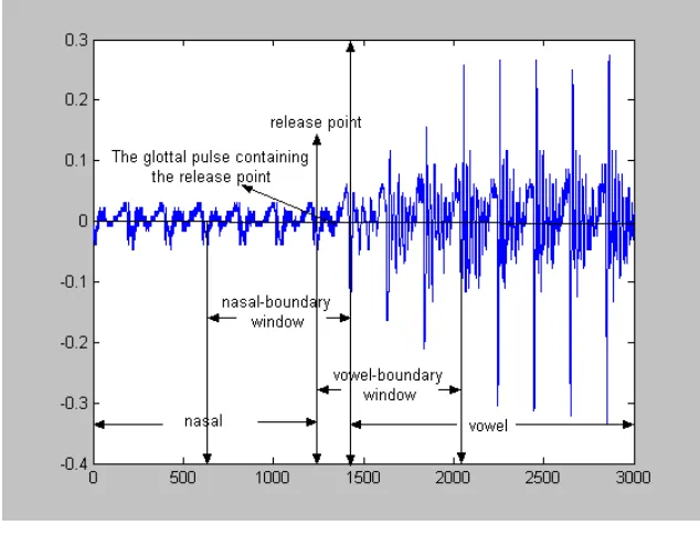
pattern of nasal pulses, and in the beginning of high-frequency components. Figure 3.1 shows

an example of the waveform display of /ma/. The release point is labeled using the arrow in

the middle of the figure. It is defined as the beginning of a pitch period that contains the first

glottal pulse (called GP1) with incipient high-frequency energy. In addition to using visual

inspection of the waveform display, LPC (Linear Prediction Coding) can help determine the

release point. If there is a change in the pattern of spectra, particularly in comparison to the

spectral pattern of the preceding nasal pulses, the current pulse is set to be the GP1 and its

starting sample to be the release point. Finally, perceptual testing can also be used to

double-check the results. In particular, the author listened to the recorded voices containing the

vowel transitions to determine whether a nasal consonant was perceived. For more details on

release point, refer to [2] and [3].

For most voice samples in the experiment, visual inspection and perceptual testing are enough to determine the release point. Moreover, the glottal pulse tracker described in [11] and [12] produces spikes wherever it goes through the release point, so it acts as an automatic way to locate release points.

The definitions of Hamming windows, such as nasal-boundary and vowel-boundary

windows, are also the same as those described in [1]. However, instead of using a fixed

length of 25.6 ms (512 samples) and 10 ms (200 samples) offset for every window, here the

windows are three glottal pulses long with one glottal pulse offset. Using fixed lengths and

offsets will result in considerable leakage when computing Fourier Transforms since the

period can be slightly incorrect. The sounds are segmented manually so that they have

Figure 3.1

Release Point, the Nasal-boundary and the Vowel-boundary Windows

1. Training and Testing

Before any statistical classification method can be implemented using the decision rules

based on (Gaussian) probability densities, the means and covariance matrices for each class

must be established. This is the training phase of the experiment. Having done this, the

model can be used to classify speech samples, which is the testing phase of the experiment.

Before the experiment, the researchers must know the class that each sound belongs to since

the result of the classification need to be verified to determine whether the model performs

well.

more details.

For each speaker, there are 200 voice files. The files were segmented carefully. Part of

the resulted sounds is taken to be the training sounds, and the rest to be the testing sounds.

Notice that the training data is required to contain equal number of different kind of

nasal-vowel combinations, such as /am/, /im/ and /um/.

2. Pre-emphasis

In 1971, Rosenberg did some perceptual experiments on glottal waveforms [25]. From his experiments, he found the spectrum falls at a rate of about 12 dB per doubling of frequency, or 12 dB/octave.

We also notice there are considerable losses to the acoustic energy in the vocal tract

during speech sound production. One type of loss, energy loss, results when the acoustic

energy radiates from the lips and nostrils in sound production. It causes a lowering of the

resonance center frequencies and an increase in the bandwidths, especially in higher

frequencies. Meanwhile, the loss produces one 6 dB/octave boost to the spectrum.

When the source spectrum is combined with the vocal tract (filter) to produce the

spectrum of the sound, peaks occur at those harmonics that are closest to the formant

frequencies of the vocal tract. The combination of the -12 dB trend caused by the source

spectrum and the +6 dB boost produces a net downward sloping spectrum of -6 dB/octave.

In the spectral analysis of voiced speech, the -6 dB/octave trend is often compensated

for by a pre-emphasis factor of +6 dB/octave to remove the downward trend. In this way, the

intensity of high frequencies will not be very low because of the downward sloping

spectrum.

The easiest way to do pre-emphasis is to subtract a scaled and delayed version of the

than 1. Typically, 0.96£a£0.99. Thus, if the signal isI(n), an approximate 6 dB/octave

rise can be obtained from the filter (3.1)

O(n)=I(n)-aI(n-1). (3.1)

Since no pre-emphasis was done in [1], however, we omit this step in this thesis. Another reason is that we mainly use the information derived from lower frequencies instead of higher ones in the computation. More specifically, the highest frequencies we consider are only in bark 22, which is centered at 8500 Hz (See the following section). Hence we ignore pre-emphasis.

For more details on pre-emphasis, refer to Chapter 3 and 6 of [25].

3. Bark Frequency Scale

This scale was developed to capture the sensation of pitch differences in terms of

"critical bands", which correspond linearly to length along the cochlea (1 critical band is

equal to a distance of 1.3mm along the basilar membrane).

In this scale, equal distances correspond with perceptually equal distances so the bark

scale represents the ability of the human ear to distinguish different tones at different

frequencies. The use of the bark scale has the effect of stretching the vowel space where the

human ear is most sensitive and contracting the space where tonal differences are difficult for

the ear to perceive. The bark scale ranges from 1 to 24 Barks, corresponding to the first 24

critical bands of hearing. The published Bark band edges are given in Hertz as [0, 100, 200,

300, 400, 510, 630, 770, 920, 1080, 1270, 1480, 1720, 2000, 2320, 2700, 3150, 3700, 4400,

5300, 6400, 7700, 9500, 12000, 15500]. The published band centers in Hertz are [50, 150,

250, 350, 450, 570, 700, 840, 1000, 1170, 1370, 1600, 1850, 2150, 2500, 2900, 3400, 4000,

4800, 5800, 7000, 8500, 10500, 13500].

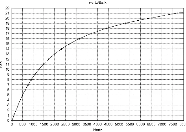
standard rounded bark scale. We can also notice that, above about 500 Hz, bark scale is similar to a logarithmic frequency axis; below 500 Hz, the scale becomes more and more linear.

The Traunmüller's approximation is defined as:

B=26.81/(1+(1960/ freq))-0.53 (3.2)

where Bis in bark, freq in Hertz.

Figure 3.2

Bark Scale VS Frequency in Hertz

We will use one example to illustrate more clearly the relationship between bark scale

and frequencies. Consider the following two figures. Figure 3.3 shows a spectrum; Figure 3.4

shows the bark scale counterpart of the spectrum. We can see that the shapes of the two

representations are not alike at all. Now let's look at the process to transform a frequency to a

bark scale. In Figure 3.3, when the coordinate of the horizontal axis takes 30 units, the

magnitude is about 75. Notice the Nyquist frequency is 2050*(1/2) =11025 Hz, and there are

128 units totally in this range (See the horizontal axis in Figure 3.3). Then, every unit in the

according to Figure 3.2. That explains the peak around bark 15. This peak is shown in Figure

3.4.

Amplitude

Frequency/86

Figure 3.3

A Spectrum of Length 128 under a Sampling Rate of 22050Hz

Amplitude

Bark

Figure 3.4

The 22 Bark-scale Representation of the Above Spectrum

PCA is widely used in data analysis and dimensionality reduction. It is a data-reduction

method that finds an alternative set of parameters for a set of utterances such that most of the

variability in the data is compressed down to the first few parameters. The transformed

dimensions in PCA are called principal components, and the new dimensions are guaranteed

to be orthogonal and uncorrelated. Briefly speaking, for a zero-mean random vector x of

dimension d, PCA tries to find k (k £d) orthonormal vectors so that the inner product of

the random vector and the individual othonormal vector will have the largest variance. It can

be shown that the k orthonormal vectors a1,a2,...,ak can be calculated by choosing the k

eigenvectors corresponding to the k largest eigenvalues of E(xxT), which is the covariance

matrix of x since E(x)=0. The k orthonormal vectors form a basis of a subspace of Rd,

and when x is projected to this subspace, it can be proved that the resulted random vector yis "closest" to x (the mean square error of y-x is minimum) over the projection of x on

any other subspace of Rd spanned by k orthonormal vectors. The PCA-derived vector

k

R Œ

w computed from xŒRd is referred to as the vector of k projection coefficients of x

on the k eigenvectors a1,a2,...,ak, so w =[a1,a2,...,ak]Tx. This PCA-derived vector has

components with the largest variances, so it can extract most of the randomness of the

original vector.

For more theory and graph representations about PCA, refer to Chapter 9.6 of [25].

In the next section, we will talk about the implementations of PCA for the Combined

Spectra method.

3.2 Algorithm, Result and Discussions

The following algorithm is based on Harrington [1]:

Calculate the spectra from the nasal-boundary windows and vowel boundary windows.

Apply no pre-emphasis. Normalize the resulting spectral values obtained from each separate

FFT by dividing them by the spectral value of the largest amplitude. Calculate the energy

values in the first 22 critical bands (in bark scale) from each amplitude-normalized spectrum

by summing all the spectrum values that fall within the separate critical bands.

2. Produce the combined spectra:

Create the combined spectra by concatenating 22 bark values from the nasal-boundary

spectra and another 22 bark values from the vowel- boundary spectra into a single vector of

length 44. Take these vectors of length 44 as the original feature representations. Let

n i

i, =1,...,

b be n such feature vectors for training purpose. Calculate their mean vector,

) ,..., ,

(fm₁ fm₂ fm₄₄

fm= , and standard deviation, fstd =(fstd₁,fstd₂,..., fstd₄₄).

Standardize the training data so that the resulted feature vectors, b'_i,i=1,...,n, have zero

mean and unit standard deviation. Transform the testing data h into h' using the mean and

standard deviation of the old training data, b_i,i =1,...,n, using the following formula:

44 ,..., 1 , ' = - i=

fstd fm

i i i i

h

h (3.3)

where h =(h1,h2,...,h44) is the original testing data; h =' (h'1,h'2,...,h'44) is the

standardized testing data.

Step 1 and 2 complete the process of Feature Extraction.

3. Implement PCA:

Training phase

Â

Â

j j j

N C N C ) 1 ( ) 1 (

, j =1,2 (3.4)

where Cj is the estimate of the covariance matrix of class j; Njis the number of sounds of

class j. Next, we calculate the corresponding eigenvalues. Discard a certain amount

(actually, 44-k, where k is the number of the largest eigenvalues defined in Section 3.1.4)

of the smallest eigenvalues and their corresponding eigenvectors. Regard the rest of the

eigenvectors as the columns of a matrix V . V =[a₁,a₂,...,a_k]. Here, a_i,i=1,...,k are the

eigenvectors we keep and k is the number of such vectors. We know that k can be any

number between 1 and 44. Then the PCA-derived feature vectors for training purpose can be

calculated as follows:

n i

VT _i i

PCA _{' , 1,...,} =

= b

b (3.5)

where bPCAi,i=1,...,n, are the PCA-derived training feature vectors. Calculate the class

centroids, mcentroidj ,j=1,2, for each nasal class by taking the mean for the PCA-derived

training feature vectors in this class. Note that the dimension of b'_i is 44, while that of bPCAi

is k.

Testing phase

Transform the testing data h' one more time using the same matrix V derived from the

training stage. Use the same transformation described in (3.5) to obtain PCA-derived testing

feature vector hPCA:

'

h

hPCA =VT (3.6)

Next, we will determine whether the sounds belong to class /m/ or class /n/ using the

4. Calculate Mahalanobis distance:

Assume our data are Gaussian distributed so that we can use the Mahalanobis distance measure [35].

The Mahalanobis distance ris defined as follows:

2 ( ) 1( centroid) j PCA j

T centroid j

PCA _{m C m}

r = h - - h - (3.7)

wherehPCA is the PCA–derived testing feature vector obtained from (3.6), mcentroid_j is the

centroid for class

j

5. Classify the testing sound:

We classify a testing sound the following way:

Calculate its Mahalanobis distance from its hPCA to each of the two class centriods; find the

smaller one; classify the sound to the class whose centroid is “nearer” to hPCA.

6. Apply experiments on different dimensions:

Repeat the above processes using different k, while k ranges from 1 to 44. Evaluate the

performance for each case.

In our experiments, we segment the data files carefully so that the experimental objects

have only 5 glottal pulses (two are nasal glottal pulses, two are vowel glottal pulses, and one

contains the release point between the nasal and vowel). In the current stage, syllable-initial

and syllable-final cases are tested separately so that the results can be more comparable to

those in [1]. After combining the sound files obtained from all the five speakers, we have 342

sounds for /m/ and 389 sounds for /n/. For each nasal consonant, 150 sounds were taken as

The result is shown in the following Figures:

Accuracy

0 5 10 15 20 25 30 35 40 45 0.4

0.5 0.6 0.7 0.8 0.9 1

Number of Dimensions Used in PCA

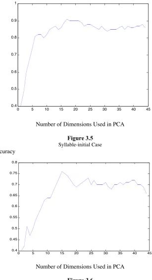
Figure 3.5 Syllable-initial Case Accuracy

0 5 10 15 20 25 30 35 40 45 0.4

0.45 0.5 0.55 0.6 0.65 0.7 0.75 0.8

Number of Dimensions Used in PCA

In the above figures, the horizontal axis is k, the number of dimensions used in PCA;

the vertical axis is the accuracy achieved when using the k eigenvectors corresponding to the k biggest eigenvalues with k between 1 and 44.

As seen, for syllable-initial case, when the first 17 eigenvectors are used, the

classification score, 91%, is the best; whereas for syllable-final case, when the first 15

eigenvectors are used, the classification score, 76%, is the best. Those results are compatible

with those of Figure 6 in Harrington [1]. We notice that the score in syllable-final case is not

as good as that in [1], which are 94% and 82%, respectively. This is probably because our

training data set is not as big as in [1] to produce a very accurate estimation of class

representation.

We also notice that when too many eigenvectors are added, the classification scores for

both cases become worse. There are two explanations:

1. When the number of eigenvectors increases, the dimension of the feature vector

increases accordingly. While the training data set does not expand, the usefulness of

each additional component is lessened. From a statistical perspective, the goodness of

fit of a Gaussian model depends on having a large number of training sounds to

estimate accurately the mean and covariance matrix. The model could be less

accurate if the number of sounds is not increased while the number of components is

increased since there could be more dependence between the components (See

chapter 9 of [25]);

2. Variations from the new added directions might not provide more information on the

identification; on the contrary, they may bring negative effects.

From this view, it is suggested that, given the fixed number of training data, we might

1. Calculate the correlations between the components and merge the highly correlated

ones in order to ensure the independence of the rest;

2. Add new, independent and useful parameters into the model so that we can have more

valuable information on the identification.

The validations of those two ideas involve discussions and theory supports on statistics,

which will be discussed in Chapter 5.

In the next chapter, Chapter 4, we will talk about some DSP methods. Those methods

extract reliable feature representations, which could be used as new parameters in the feature

Chapter 4

Feature Extraction

Using

Singular Value and Eigenvalue Tests

In the Combined Spectra Method, the classification model was established using a

feature vector of length 44, which is derived from the spectra around the transition regions of

the nasal sounds. In this chapter, new feature parameters will be extracted which could be

added into the feature vector as new components. We attempt to produce higher classification

scores. The theoretical support and implementation of this idea is introduced in the next

chapter. In this chapter, we discuss the extraction of the new features.

Our feature extraction approaches are based on singular-value and eigenvalue tests.

Those approaches can successfully extract useful information on differences between nasals.

4.1 Singular Value Tests

Definitions

The Singular Value Decomposition (SVD) of a rectangular n by m matrix A is defined as

T

USW

A= (4.1)

where U is an n by n left orthogonal matrix, W is an m by m right orthogonal matrix and S

is an n by m diagonal matrix of non-negative singular values. The columns of U form an orthonormal basis for the space spanned by the columns of A, while the columns of W form

an orthonormal basis for the space spanned by the rows of A. The columns u_i and w_i of

Uand W are called the left and right singular vectors, respectively. The singular values, s_j,

The properties of SVD are similar to those of the better-known eigenvalue decomposition. They both decompose the input matrix into a set of orthonormal basis matrices. SVD differs from the eigenvalue decomposition in that it is valid for any input matrix, while the eigenvalue decomposition is only defined for square matrices. Both SVD and the eigenvalue decomposition have been widely used to separate an input signal’s spectrum into signal and noised components. SVD has one more advantage in that it can always give a real valued solution if the input matrix is real, whereas the eigenvalue decomposition may give a complex solution.

The SVD has a variety of applications in scientific computing, signal processing,

automatic control, and many other areas. One important application on signal processing is

Matrix Approximation:

By neglecting the small singular values in the "middle matrix" S in the SVD, we can obtain matrix approximations whose rank equals the number of remaining singular values. Since the singular values appear in decreasing order, the formula for the matrix approximation becomes

T k k k T

k u s w u s w

A = 1 1 1 +...+ (4.2)

where kis the number of retained singular values. The terms u_is_iw_iT are called the principal

images. Often very accurate matrix approximations can be obtained with only a small fraction of the singular values.

Other applications of the SVD include computational tomography, image de-blurring, and geophysical inversion (seismology).

Application to Nasals

In this section, the SVD technique is used to try to distinguish nasals since the singular

values are alternatives to frequencies, and it is expected that they can perhaps show

Since the cues of place of articulation lie in the transition part between the vowels and

nasals, the algorithm is implemented in the transition regions of the voice samples.

In Chapter 3, the experiments were conducted on a set of data recorded from different speakers. In this chapter, we use voice samples recorded from only one speaker since the automated system requires nasal identification of a single speaker.

After we locate the release point, as we did in Chapter 3, we take only five glottal pulses around it for our experiment to avoid the huge computation caused by calculation for singular values of an N by N matrix (defined next), where N is a large number (We will see later that usually N> 150). Those five glottal pulses are: GP1, two glottal pulses before GP1 and two after it. They are segmented carefully by hand so that we can estimate periods of the glottal pulses accurately. See Figure 4.1.

0 500 1000 1500 2000 2500 3000

-0.4 -0.3 -0.2 -0.1 0 0.1 0.2 0.3

release point

nasal

vowel ma.wav

GP1 Beginning of GP1

5 glottal pulses

Figure 4.1

Release Point and the Five Glottal Pulses

If a glottal pulse contains approximately 200 samples, 5 glottal pulses is about 200*5/22050=0.045 seconds in duration where 22050 Hz is the sampling rate. Hence, we are

experimenting on a very short nasal-vowel transition signal.