Searching the Hyperparameter Space for
Tuning of Neural Networks
Aishwarya Radhakrishnan1
BE Student, Department of Information Technology, Mumbai University, Vivekanand Education Society’s Institute of
Technology, Mumbai, India 1
ABSTRACT: An experiment was performed using a two-layer neural network for pattern classification/character recognition.The learning cost for two-layer backpropagation networks is examined in the context of learning non-linear equations from examples. In particular, the relationship between the number of inputs, hidden units, regularization parameter , number of iterations and training set vectors is investigated. The networks, the training algorithm, and the tasks are described. The parameter variations and the set of simulations performed are detailed. Orthogonalization and early stopping method is discussed and then the hyperparameter space is explored to see if our model selection was correct and the simulation results are summarized.
KEYWORDS: Optical Character Recognition (OCR), Neural Network(NN), Amazon Web Services(AWS)
I. INTRODUCTION
The human visual system is one of the wonders of the world. Consider the following sequence of handwritten digits:
Figure 1 Handwritten digits
Most people effortlessly recognize those digits as 504192. That ease is deceptive. In each hemisphere of our brain, humans have a primary visual cortex, also known as V1, containing 140 million neurons, with tens of billions of connections between them. And yet human vision involves not just V1, but an entire series of visual cortices - V2, V3, V4, and V5 - doing progressively more complex image processing. We carry in our heads a supercomputer, tuned by evolution over hundreds of millions of years, and superbly adapted to understand the visual world. Recognizing handwritten digits isn't easy. Rather, we humans are stupendously, astoundingly good at making sense of what our eyes show us. But nearly all that work is done unconsciously. And so we don't usually appreciate how tough a problem our visual systems solve.
The difficulty of visual pattern recognition becomes apparent if you attempt to write a computer program to recognize digits like those above. What seems easy when we do it ourselves suddenly becomes extremely difficult. Simple intuitions about how we recognize shapes - "a 9 has a loop at the top, and a vertical stroke in the bottom right" - turn out to be not so simple to express algorithmically. When you try to make such rules precise, you quickly get lost in a morass of exceptions and caveats and special cases. It seems hopeless.
II. RELATED WORK
Perceptrons were developed in the 1950s and 1960s by the scientist Frank Rosenblatt, inspired by earlier work by Warren McCulloch and Walter Pitts. Today, it's more common to use other models of artificial neurons - in the book “Principles of neurodynamics”, and in much modern work on neural networks, the main neuron model used is one called the sigmoid neuron.Obviously, the perceptron isn't a complete model of human decision-making! But a perceptron can weigh up different kinds of evidence in order to make decisions. And it should seem plausible that a complex network of perceptrons could make quite subtle decisions.Since 2006, a set of techniques has been developed that enable learning in deep neural nets.Instead, we'd like to use learning algorithms so that the network can automatically learn the weights and biases - and thus, the hierarchy of concepts - from training data. Also, instead of training the model with many iterations and overfitting the training set we can use early stopping it stop the training before when the fit of the hypothesis to the data is “just right”.Most common learning algorithms feature a set of hyperparameters that must be determined before training commences.The choice of hyperparameters can significantly affect the resulting model’s performance, but determining good values can be complex. The combination of all the possible values of hyperparameter makes hyperparameter search a formidable optimization task.
III. THE GOAL OF THIS PAPER
In order to improve the generalization ability of neural networks, many algorithms have been devised such as adding a regularizer to the original criterion function with the aim to reduce the complexity of weight matrix and get sparse weight matrix of neural networks. In this paper we explore the hyperparameter space to get a sense of the behaviour of 2 layered Neural Network when it’s hyperparameters are changed.
IV. SIMULATION METHOD
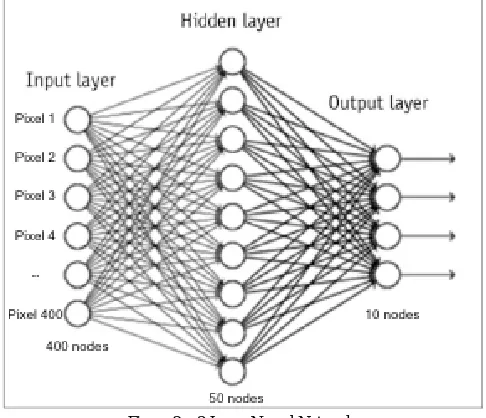
When we count the number of layers in a neural network, we only count the layers with connections flowing into them (omitting our first, or input layer). So the below figure is of a 2-layer neural network with 1 hidden layer.
Figure 2: 2 Layer Neural Network
When creating a machine learning model, you'll be presented with design choices as to how to define your model
of searching for the ideal model architecture is referred to as hyperparameter tuning.These hyperparameters might address model design questions such as:
1. What degree of polynomial features should I use for my linear model?
2. What should be the maximum depth allowed for my decision tree?
3. What should be the minimum number of samples required at a leaf node in my decision tree?
4. How many trees should I include in my random forest?
5. How many neurons should I have in my neural network layer?
6. How many layers should I have in my neural network?
7. What should I set my learning rate to for gradient descent?
The hyperparameter space is checked in by implementing Backpropogation algorithm using MATLAB and Octave. For continuous training, it’s possible to transfer the load of training the model on low memory pc to Amazon Web Services instance. Basically, any device with a screen and an Internet connection can access high-powered computing such as AWS. So in order to run MATLAB and Octave code on AWS instance, we need to install Octave on AWS instance.
Steps to install Octave on AWS instance and run octave code are as follows:
1. Install EPEL:
sudo yum install https://dl.fedoraproject.org/pub/epel/epel-release-latest-$(rpm -E '%{rhel}').noarch.rpm
2. List your repos :
sudo yum repolist
3. Search package in epel repository:
sudo yum --disablerepo="*" --enablerepo="epel" list available | grep 'octave'
4. Search and install Octave:
sudo yum search octave ## get more info, if found ## sudo yum info octave
sudo yum install octave
5. Copy files from local machine to AWS instance by running the command from local machine:
scp -i "/Users/local/machine/securitycertificate.pem file1.mat file2.m user@ec2hostname:/home/ubuntu/myproject
6. Invoking Octave from the Command Line:
octave
7. Run octave commands.
8. Exit the current Octave session:
exit #or quit
9. Exit AWS instance:
V. THEORETICAL FOUNDATIONS
The dataset is split into training set , cross validation set and test set. We then use the training set to fit our parameters using the Backpropogation algorithm. Once the parameters are fit, we then choose a model either using orthogonalization or early stopping method. But, later in this paper, we will see how we can check the hyperparameter space to see if our model selection was correct.Backpropagation is a method used in artificial neural networks to calculate a gradient that is needed in the calculation of the weights to be used in the network. It is commonly used to train deep neural networks,a term referring to neural networks with more than one hidden layer.Loss function sometimes referred to as the cost function or error function, the loss function is a function that maps values of one or more variables onto a real number intuitively representing some "cost" associated with those values. For backpropagation, the loss function calculates the difference between the network output and its expected output, after a case propagates through the network.The optimization algorithm repeats a two phase cycle, propagation and weight update. When an input vector is presented to the network, it is propagated forward through the network, layer by layer, until it reaches the output layer. The output of the network is then compared to the desired output, using a loss function. The resulting error value is calculated for each of the neurons in the output layer. The error values are then propagated from the output back through the network, until each neuron has an associated error value that reflects its contribution to the original output.Backpropagation uses these error values to calculate the gradient of the loss function. In the second phase, this gradient is fed to the optimization method, which in turn uses it to update the weights, in an attempt to minimize the loss function.
The concrete steps of backpropagation algorithm are composed of the following steps: 1. Forward pass from input layer to output layer.
2. Backward pass error signal from output layer to input-layer 3. Update the weights.
The basic steps after backpropagation as described above is only one important processing step that is added in the above description. This added step is described in detail as follows. After converging the parameters Theta using advanced optimization method, we can plot cost as a function of no of iteration for training and cross validation. If the training cost is less (i.e. does not underfit the data) but the gap between the training error and cross validation error is large, the learning algorithm fails to generalized to new examples. Thus, in order to deal with such over fitting problem we can use Regularization techniques. We can use Regularization parameter (lambda) and change this hyperparameter value to achieve a hypothesis that can generalize well on the cross validation set. Using Dropout Regularization will be another Regularization technique. Tuning these hyperparameter that let the training set converge is called Orthogonalization.
Another concept is, early stopping where we regularize without using orthogonalization i. e. we do not let the algorithm converge and without a converged algorithm we tune one of our hyperparameter. When we iterate over the training set and crossvalidation set, for training set initially the cost is high and as the number of iteration increases the cost decreases while for cross validation set initially the cost is very high but as the number of iterations increases, the cost decreases but does not reach close to training set cost. The gap between training set error and cross validation set error is large. There is a point where the gap between training set error and cross validation set error is close after which the training set error declines while the cross validation set error does not decline as steeply. This point is called early stopping. Conceptual if we stop at this point, then we should get the difference between training set error and cross validation set error to be small. But in early stopping, we do not let the algorithm to converge. Following steps can be performed to manually perform early stopping:
1. Run Neural Network (NN) for far more time 2. Save the model weights every N epochs
Validation can be used to detect when overtting starts during supervised training of a neural network; training is then stopped before convergence to avoid the overfitting (or perform early stopping). The exact criterion used for validation-based early stopping, however, is usually chosen in an ad-hoc fashion or training is stopped interactively.
VI.WHY EARLY STOPPING?
When training a neural network, one is usually interested in obtaining a network with optimal generalization performance. However, all standard neural network architectures such as the fully connected multi-layer perceptron are prone to overfitting. While the network seems to get better and better, i.e., the error on the training set decreases, at some point during training it actually begins to get worse again, i.e., the error on unseen examples increases. The idealized expectation is that during training the generalization error of the network evolves. Typically the generalization error is estimated by a validation error, i.e., the average error on a validation set , a set of examples not from the training set. There are basically two ways to prevent overfitting: reducing the number of dimensions of the parameter space or reducing the effective size of each dimension. Techniques for reducing the number of parameters are greedy constructive learning , pruning , or weight sharing. Techniques for reducing the size of each parameter dimension are regularization, such as weight decay and others, or early stopping. Early stopping is widely used because it is simple to understand and implement and has been reported to be superior to regularization methods in many case.
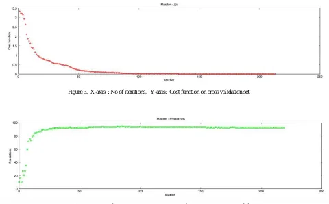
Figure 3. X-axis : No of iterations, Y-axis: Cost function on cross validation set
Figure 4. X-axis : No of iterations, Y-axis: Correct Prediction Percent on cross validation
claimed to show the evolution over time of the validation error on the validation set. Given this behavior, it is clear how to do early stopping usingvalidation error.
1. Split the training data into a training set and a validation set, e.g. in a 2-to-1 proportion.
2. Train only on the training set and evaluate the per-example error on the validation set once in a while, e.g. after every fth epoch.
3. Stop training as soon as the error on the validation set is higher than it was the last time it was checked. 4. Use the weights the network had in that previous step as the result of the training run.
This approach uses the validation set to anticipate the behavior in real use (or on a test set), assuming that the error on both will be similar. The validation error is used as an estimate of the generalization error.Figure 3 shows the cost function on cross validation set which seems to be same after 75 iteration and so does prediction percent on cross validation after 50 iteration. But if we zoom in to get the plot from 75 iteration to 220 iteration , we get the plots in figure 5 and figure 6 below.
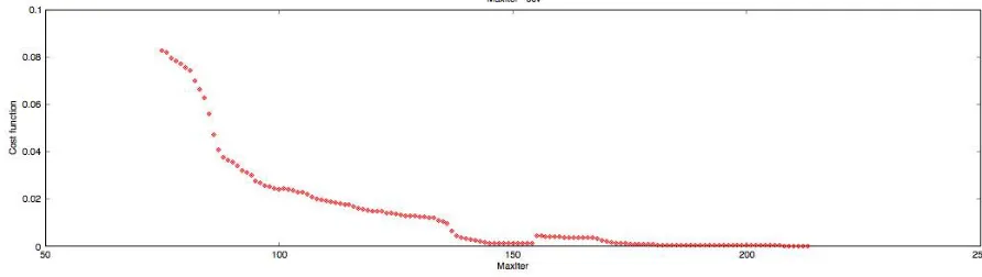
Figure 5. X-axis : No of iterations, Y-axis: Cost function on cross validation set
Figure 6. X-axis : No of iterations, Y-axis: Correct Prediction Percent on cross validation
It means that the training set has overfit the data. Instead of overfitting it till 220 iteration, we can achieve a good prediction error at an optimal stopping point of 75 iteration. Thus stopping the iteration at 75 would be called early stopping.Note that stopping in iteration 220 compared to stopping at iteration 75 trades an about threefold increase of learning time for an improvement of validation set error by 0.0827 and for a decrease inprediction percent on cross validation by 0.94%. This decrease in prediction percent is however indicative of overfitting as the model has overfit
the data and hence it’s prediction on new data becomes worse.Unfortunately, the above or any other validation error
curve is not typical in the sense that all curves share the same qualitative behavior. Other curves might never reach a better minimum than the first, or than, say, the third; the mountains and valleys in the curve can be of very different width, height, and shape. The only thing all curves seem to have in common is that the differences between the first and the following local minima are not huge. As we see, choosing a stopping criterion predominantly involves a tradeoff between training time and generalization error. However, some stopping criteria may typically find better tradeoff that others. So, we set the optimal stopping iteartion at 75 iteration.
VII. HYPERPARAMETER TUNING
The same kind of machine learning model can require different constraints, weights or learning rates to generalize different data patterns. These measures are called hyperparameters, and have to be tuned so that the model can optimally solve the machine learning problem. Hyperparameter optimization finds a tuple of hyperparameters that yields an optimal model which minimizes a predefined loss function on given independent data. The objective function takes a tuple of hyperparameters and returns the associated loss. Cross-validation is often used to estimate this generalization performance.
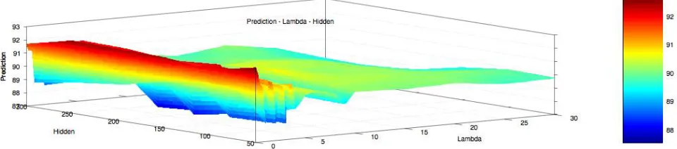
Figure 7. X-axis : Number of hidden nodes in layer 1, Y-axis: lambda, Z-axis: Cost function on cross validation set
Figure 8. X-axis : Number of hidden nodes in layer 1, Y-axis: lambda, Z-axis: Correct Prediction Percent on cross validation set
percentage is plot in figure 8. Searching the hyperparameter space keeping maximum number of iterations equal to 50 and number of training examples equal to 3750 and by iterating over possible values of lambda and number of hidden units of neural networks in figure 7 and 8, 50 hidden unites, lambda equal to 0 gives best prediction on cross validation set. This result is got by iterating over the 6 possible values of hidden units and 32 possible values of lambda giving a total of 186 combinations. In these, the prediction was equivalently high at 50 hidden units compared to 200 or 300 hidden units. And the cost was low at 50 hidden units. Both these properties i.e. low cost on cross validation set and high percentage of correct predictions made occur at lambda equal to 0. So if we vary cost on cross validation set as a function of number of hidden units and lambda, in this problem we get 50 hidden units and lambda equal to 0 as best hyperparameter values for a training set of 3000 examples and 400 features from a 20x20 image dataset. Worst performance is given by 3000 hidden unites and lambda 0 which seems valid since the number of hidden units increase will overfit the cross validation set if the regularization parameter is 0.
Figure 9. X-axis : Number of hidden nodes in layer 1, Y-axis: lambda, Z-axis: Cost function on cross validation set
Figure 10. X-axis : Number of hidden nodes in layer 1, Y-axis: lambda, Z-axis: Correct Prediction Percent on cross validation set
hyperparameter space and hence 50 hidden units and lambda as 0 can be used as a model having good predictive percentage.
Now we keep number of hidden units as 50 and lambda as 0, and vary maximum iteration and number of training examples used to get the cross validation error.
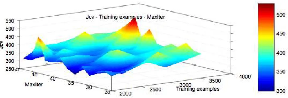
Figure 11. X-axis : Number of training examples , Y-axis: Number of Iterations, Z-axis: Cost function on cross validation set
Figure 12X-axis : Number of training examples , Y-axis: Number of Iterations, Z-axis: Correct Prediction Percent on cross validation set
Then iteration over the hyper parameter space by varying number of training examples and number of iterations is done to get the lowest cost over the cross validation set in figure 11 and highest prediction percentage over the cross validation set in figure 12. On varying the no of training examples from 2000 to 4000 and maximum iterations from 25 to 50, the prediction reaches it's peak when maximum iteration is 37 and training examples is 3500 as in figure 12 while cost on cross validation set is minimum when training examples is 2000 and maximum iterations is 35 as in figure 11. Thus, if we choose a training model having hyperparameter value of number of iterations within 30 to 50 and and training examples close to 3500 we can then get a good generalization from our model.
VIII. CONCLUSION
Thus, we can conclude that on searching the hyperparameter space we can get a glimpse of how the trained model
evolves from underfitting to “just right” fit to overfitting. And also we have seen how we can use early stopping to stop
values based on the experiments building models with various hyperparameter values and recording the model performance for each combination of hyperparameter.
REFERENCES
1. Mark Schmidt. Machine Learning Lecture 1 Introduction - Cs.ubc.ca. CS540University of British Columbia. January-April, 2018 2. Michael Nielsen. Using neural nets to recognize handwritten digits.neuralnetworksanddeeplearning.com Sep 2018
3. Szu, US Naval Res. Lab., Washington, DC, USA. “Gram-Schmidt orthogonalization neural nets for OCR”. Ieee Xplore Digital Library. September 4th, 2015
4. T. E. de Campos, B. R. Babu and M. Varma. Character recognition in natural images. In Proceedings of the International Conference on Computer Vision Theory and Applications (VISAPP), Lisbon, Portugal, February 2009.
5. Weishui Wan, Kotaro Hirasawa, Jinglu Hu. Enhancing the Generalization Ability Of Neural Networks By Using Gram-Schmidt Orthogonalization Algorithm. Volume 39 (2003) Issue 7. Jstage. 2003
6. Ian Goodfellow, Yoshua Bengio, Aaaron Courville; Deep Learning; MIT Press; p 1962016
7. Nielsen, Michael A. "Chapter 6". Neural Networks and Deep Learning.neuralnetworksanddeeplearning.com 2015 8. Andrew NG, Jngiam, Cyfoo, Watsuen. "Deep Networks: Overview - Ufldl". ufldl.stanford.edu. Retrieved 2017-08-04. 9. Claesen, Marc; Bart De Moor. "Hyperparameter Search in Machine Learning". arXiv:1502.02127 [cs.LG].2015
10. Bergstra, James; Bengio, Yoshua. "Random Search for Hyper-Parameter Optimization" (PDF). J. Machine Learning Research. 13: 281– 305.2012
11. Jeremy Jordan. Hyperparameter Tuning For Machine Learning Models. 2 November 2017