ABSTRACT
SATCHER, MELINDA RENEE. De-bottlenecking the Electrospinning Process Using
Superparamagnetic Particles. (Dr. Juan Hinestroza and Dr. Saad Khan.).
Nanocomposite polyethylene oxide (PEO) fibers containing magnetic domains were
produced using parallel plate electrospinning. The fibers were spun from solutions dosed
with nanoparticles of magnetite (Fe3O4) in 2wt% PEO in water. Solution parameters like
viscosity, conductivity, and surface tension were measured and correlated to final fiber
diameter. Increased amounts of magnetic nanoparticles produced higher conductivity,
higher viscosity, and lower surface tension solutions.
Transmission electron microscopy and energy dispersive spectroscopy were used to
analyze the diameters of the nanofibers as well as the distribution of the magnetic
nanoparticles inside the PEO matrix. A SQUID magnetometer was applied to determine
the AC and DC magnetic susceptibility of the fibers. The resultant nanofibers had
diameters as low as 100 nm and exhibited unique AC susceptibility patterns and magnetic
responses making them excellent for anti-counterfeiting applications.
DE-BOTTLENECKING THE ELECTROSPINNING PROCESS USING SUPERPARAMAGNETIC PARTICLES
by
Melinda Renee Satcher
A thesis submitted to the Graduate Faculty of
North Carolina State University
In partial fulfillment of the
Requirements for the degree of
Master of Science
In
Textile Engineering
Raleigh, NC
2006
Approved by:
Dr. Juan Hinestroza Co-Chair of Advisory Committee
Dr. Saad Khan
Co-Chair of Advisory Committee
Dr. William Oxenham Committee Member
DEDICATION
This work is dedicated to my father, the late Larry Satcher. My father passed away in
November of 2005 while I was working on this research. His love and encouragement
are the only reasons I finished this thesis.
BIOGRAPHY
Melinda Renee Satcher was born in November of 1979 in Macon, GA to Larry and
Barbara Satcher. Melinda is the youngest of three children; she has an older brother and
sister. After graduating from Southwest High School, Melinda enrolled in the Regent’s
Engineering Transfer program between Georgia Southern University and the Georgia
Institute of Technology. She completed two years at GSU, before transferring to Georgia
Tech pursuing a B.S. in Chemical Engineering. While in college, Melinda completed
undergraduate research for the Polymer Manufacturing Research Center, focusing on
post-consumer carpet recycling and polypropylene nanocomposites. After graduating in
December 2002, Melinda began a position as a Product/Process Improvement Engineer
for Milliken & Co. in the Automotive Division. At the Elm City Plant she has held two
positions, the dyeing manager for Decorative Fabrics and the dyeing manager for
Automotive Fabrics. Outside of work and school, Melinda enjoys watching football and
ACKNOWLEDGEMENTS
I would like to thank Dr. Juan Hinestroza for all of his guidance and support in
completing this project. Also I would like to thank Dr. Saad Khan and his research group
for their help. Dr. Lei Qian and Dr. William Oxenham were also important members of
my thesis committee. Dr. Carlos Rinaldi and his research group at the University of
Puerto Rico at Mayaguez were very influential in the magnetic field experiments and
magnetic characterization. Dr. Mark Walters and the Shared Materials Research Lab at
Duke University provided training and support with different microscopy techniques. Dr.
Gerardo Montero helped to train me on the electrospinning equipment and other analysis
techniques. Finally, I would like to thank the Institute of Textile Technology and
TABLE OF CONTENTS
LIST OF FIGURES... viii
LIST OF TABLES... xi
1. INTRODUCTION ... 1
1.1 BACKGROUND ... 1
1.2 MOTIVATION... 2
1.3 OBJECTIVES ... 2
2. LITERATURE REVIEW ... 3
2.1 ELECTROSPINNING... 3
2.1.1 CONCEPT ... 3
2.1.2 PARAMETER INVESTIGATION ... 6
2.1.2.1 VISCOSITY ... 6
2.1.2.2 CONDUCTIVITY ... 7
2.1.2.3 SURFACE TENSION... 8
2.1.2.4 APPLIED ELECTRIC FIELD ... 9
2.1.3 STABILITY ANALYSIS... 10
2.2 MAGNETIC NANOPARTICLES ... 11
2.2.1 CONCEPT OF MAGNETISM ... 11
2.2.2 MAGNETIC PROPERTIES... 12
2.2.3 FERROFLUIDS ... 15
2.4 FIBER ANALYSIS TECHNIQUES ... 17
2.4.1 SCANNING ELECTRON MICROSCOPY ... 17
2.4.2 TRANSMISSION ELECTRON MICROSCOPY ... 17
2.4.3 MAGNETIC ANALYSIS/ SQUID ... 19
3. EXPERIMENTAL PROCEDURE ... 20
3.1 MATERIALS... 20
3.1.1 PREPARATION OF PEO-MAGNETITE SOLUTIONS ... 20
3.1.2 VISCOSITY ... 22
3.1.3 CONDUCTIVITY MEASUREMENTS ... 23
3.1.4 SURFACE TENSION MEASUREMENTS ... 24
3.2 ELECTROSPINNING EXPERIMENTS... 25
3.3 MAGNETIC FIELD EXPERIMENTS ... 27
3.4 ANALYSIS METHODS ... 28
3.4.1 SCANNING ELECTRON MICRCROSCOPY... 28
3.4.2 TRANSMISSION ELECTRON MICROSCOPY ... 29
3.4.3 SUPERCONDUCTING QUANTUM INTERFERENCE DEVICE ... 30
4. RESULTS AND DISCUSSION ... 31
4.1 ELECTROSPINNING PHASE DIAGRAMS ... 32
4.2 FIBER CHARACTERIZATION... 35
4.2.1 FIBER DIAMETER ... 35
4.2.2 ENERGY DISPERSIVE SPECTROSCOPY ... 41
4.3.1 SQUID HYSTERESIS ... 44
4.3.2 SQUID AC SUCEPTIBILITY ... 47
4.4 ALTERNATING MAGNETIC FIELD... 49
5 CONCLUSIONS... 53
6 SUGGESTIONS FOR FURTHER RESEARCH... 54
7 REFERENCES ... 58
APPENDICES ... 63
APPENDIX A: CALCULATIONS ... 64
LIST OF FIGURES
Figure 1 Main components of electrospinning set-up... 4
Figure 2 Depiction of three phases of flow in electrospinning... 5
Figure 3 Hysteresis curve example ... 14
Figure 4 Transmission microscope schematic [45] ... 18
Figure 5 TEM micrograph of magnetite particles in the MSG W11 ferrofluid... 21
Figure 6 Distribution histogram of magnetite particle size in MSG W11 ferrofluid... 21
Figure 7 AR2000 Viscosity profiles for PEO/water, 0.01 v/v magnetite/ PEO, 0.10 v/v magnetite/PEO, and pure MSG W11 ferrofluid ... 23
Figure 8 Conductivity Measurements for PEO/water, 0.01 v/v magnetite/ PEO, and 0.10 v/v magnetite/PEO ... 24
Figure 9 Surface tension measurements for PEO/water, 0.01 v/v magnetite/ PEO, and 0.10 v/v magnetite/PEO ... 25
Figure 10 NCSU laboratory electrospinning equipment ... 26
Figure 11 Schematic of NCSU laboratory parallel plate electrospinning set-up... 27
Figure 12 NCSU/UPRM laboratory electrospinning schematic with alternating magnetic field capabilities ... 28
Figure 13 Duke University Shared Materials Instrumentation Facilities Hitachi HF-2000 TEM ... 29
Figure 14 UPRM chemical engineering laboratory SQUID Magnetometer ... 30
Figure 16 PEO/water electrospinning phase diagram depicting the flow rate and electric
field for dripping, stable, and whipping flow ... 32
Figure 17 Magnetite/ PEO (containing v/v 0.01magnetite) electrospinning phase diagram
depicting the flow rate and electric field for dripping, stable, and whipping flow... 33
Figure 18 Magnetite/ PEO (containing v/v 0.10 magnetite) electrospinning phase diagram
depicting the flow rate and electric field for dripping, stable, and whipping flow... 34
Figure 19 X-bar chart of electrospun magnetite/ PEO ( containing v/v 0.01magnetite)
average fiber diameter... 36
Figure 20 X-bar chart of electrospun magnetite/ PEO ( containing v/v 0.10magnetite)
average fiber diameter... 36
Figure 21 TEM micrograph of PEO nanofiber containing 0.01 v/v magnetite
nanoparticles ... 38
Figure 22 TEM micrograph of PEO nanofiber containing 0.01 v/v magnetite
nanoparticles ... 39
Figure 23 TEM micrograph of PEO nanofiber containing 0.10 v/v magnetite
nanoparticles ... 40
Figure 24 TEM micrograph of PEO nanofiber containing 0.10 v/v magnetite
nanoparticles ... 41
Figure 25 EDS spectrograph for PEO nanofiber containing 0. 01 v/v magnetite
nanoparticles ... 42
Figure 26 EDS spectrograph for PEO nanofiber containing 0. 10 v/v magnetite
Figure 27 Room temperature hysteresis curve for electrospun PEO nanofiber containing
0.01 v/v magnetite nanoparticles ... 45
Figure 28 Room temperature hysteresis curve for electrospun PEO nanofiber containing 0.10 v/v magnetite nanoparticles ... 46
Figure 29 Out-of-phase component of the AC susceptibility for PEO nanofibers containing v/v 0.01 and v/v 0.10 magnetite nanoparticles... 47
Figure 30 Out-of-phase component of the AC susceptibility for PEO nanofibers containing v/v 0.01 and v/v 0.10 magnetite nanoparticles... 48
Figure 31 Electrospinning set-up #1 with AC magnetic field capabilities ... 49
Figure 32 Electrospinning set-up #2 with AC magnetic field capabilities ... 50
Figure 33 Electrospinning set-up #3 with AC magnetic field capabilities ... 51
Figure 34 Backward Electrospinning Schematic ... 52
Figure 35 Magnetite/ PEO (containing v/v 0.10 magnetite) electrospinning phase diagram depicting the flow rate and electric field for dripping, stable, and whipping flow using glass tip... 55
Figure 36 Recommended solenoid enclosed in dielectric material for electrospinning with AC magnetic field ... 56
LIST OF TABLES
Table 1 Magnetite Particle Diameter Mean and Std. Deviation ... 21
Table 2 Magnetite/ PEO volume fractions used in electrospinning trials ... 22
Table 3 Hitachi HF-2000 Microscope settings ... 29
Table 4 EDS summary for PEO nanofiber containing 0. 01 v/v magnetite nanoparticles 42
1. INTRODUCTION
1.1 BACKGROUND
In recent years there has been increased interest in ‘smart’ materials that are sensitive to
environmental changes and respond to external fields. These materials can alter their
properties in response to changes in the surrounding environment. Of particular interest is
the use of magnetic particles in combination with polymeric materials. The processiblity,
noncorrosive nature, and light weight features of polymers make them excellent matrixes
for magnetic particle inclusion. Magnetic nanoparticles can be embedded in polymeric
matrices to impart the resulting nanocomposite with magnetic properties like unique AC
susceptibility and hysteresis. For example, in the medical field, synthesizing drugs coated
with magnetic nanocomposites provides a way for drugs to be released in a controlled
manner using an external magnetic field [1]. Polymer nanocomposites have potential uses
in producing magnetic recording media or high-frequency applications [2-4]. The
magnetic responsiveness of these composites makes them of interest to the polymer,
biomedical, and textile industries.
Electrospinning has been identified as a process able to produce polymeric fibers at the
nanoscale level with nanoscale features. A better understanding of the operating
parameters and solution parameters may help to de-bottleneck the electrospinning process
and translate it from the laboratory to the commercial scale. The main research question
process and produce fibers with magnetic properties such as characteristic AC
susceptibility spectra?
1.2 MOTIVATION
The production of fibers at the nanoscale level is of current interest to the textile industry.
Polymer nanofibers have potential uses in protective clothing, ‘smart clothing,’
biomedical applications including would dressings and drug delivery systems, and
anti-counterfeiting specialty fibers. The proposed research is expected to identify an
alternative procedure to lower the viscosity of a polymer solution without lowering its
concentration. In addition to de-bottlenecking the electrospinning process, the use of
superparamagnetic particles can be used to develop fibers with controllable magnetic
fingerprints. These fingerprints can aid in anti-counterfeiting devices and supply a
‘signature’ for the identification of textile raw materials and finished goods.
1.3 OBJECTIVES
1. To examine the factors that control final fiber diameter during the electrospinning
process
2. To understand the effect of superparamagnetic particles on the solution properties
and operating parameters of the electrospinning process
3. To examine nanofibers morphology and magnetic properties as a function of
2. LITERATURE REVIEW
2.1 ELECTROSPINNING
2.1.1 CONCEPT
Electrospinning is a process able to generate fibers with diameters smaller than 200
nanometers. The concept of electrospinning is not new to the textile industry as the first
patent dates back to the 1930s.With increased interest in smaller fibers, research efforts
have concentrated on optimizing the electrospinning process for large-scale commercial
production. As the knowledge base of the fundamentals of electrospinning expands, the
solution viscosity has been identified as a key parameter in controlling the final fiber
diameter [5-7]. The production of smaller fiber diameters often requires the use of dilute
solutions and high power requirements, thereby limiting the production rate and
commercialization of this process.
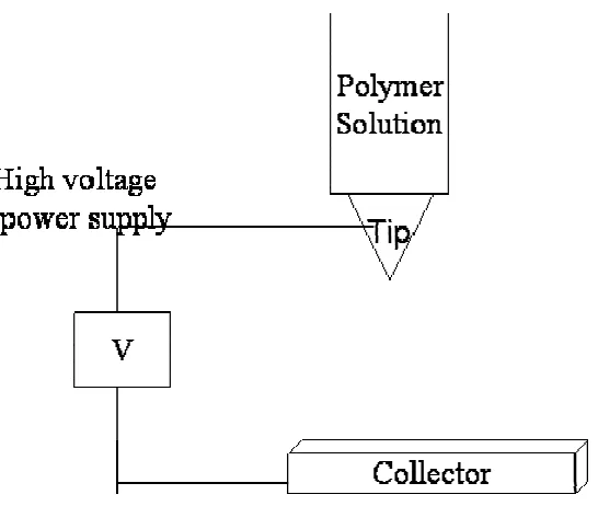
There are three major components in the electrospinning set-up: a high voltage power
supply, a solution container connected to a conductive tip, and a metal collector [5]. The
traditional process of electrospinning involves the application of high voltage to a
capillary tip [5, 7]. The positive electrode is connected to the tip and the negative
Figure 1 Main components of electrospinning set-up
The charged tip is connected to a polymer reservoir containing polymer solution. With
the use of a pump, the polymer solution is fed through the tip into the electric field
between the tip and the collector [7].
During the electrospinning process, a polymer solution is subjected to an electric field.
When the surface tension of the solution is overcome by the charge induced by the
electric field, a jet of polymeric solution is produced. As the jet leaves the tip, it takes on
the shape of a Taylor cone [7, 8]. The jet proceeds in a straight line until it begins to bend
in a zigzag pattern. During this time, the jet elongates, the solvent evaporates and
polymer nanofibers on formed [9, 10].
The process of electrospinning begins as a polymer solution is pumped into a capillary
forces elongate the jet of polymer solution, decreasing its diameter thousands or even
millions of times. After the solvent evaporates, fibers with diameters in the range of 50
-500 nanometers are then collected on an electrically grounded surface.
Unlike traditional fiber spinning techniques, electrospinning relies on electrical forces
instead of mechanical forces [6]. These forces provide the phenomenon that transforms a
drop into a jet as shown in Figure 1.
Figure 2 Depiction of three phases of flow in electrospinning
The jet thins as it heads toward the collector plate and it may experience a flow
instability, known as whipping [11, 12]. This instability leads to extensive stretching and
elongation of the jet. The whipping may decreases the fiber diameter up to 3 orders of
magnitudes [13].
The electrostatic forces are not the only forces that affect the electrospinning process.
Gravitational forces, columbic repulsive forces, viscoelastic forces, and surface tension
trajectories for the jet. For example, the columbic repulsive forces contribute to the
stretching of the jet, while the surface tension and viscoelastic forces act against it.
2.1.2 PARAMETER INVESTIGATION
As the investigation into the parameters that influence electrospinning nanofibers
continues, the following properties have been identified as the most influential in
controlling final fiber diameter: viscosity, conductivity, surface tension, and applied
electric field.
2.1.2.1 VISCOSITY
The viscous forces of a solution resist the electrical forces that attempt to stretch the fiber
during electrospinning [15]. It has been found that there exists an optimum viscosity
range for producing nanofibers [16]. At higher viscosities, the cohesiveness of the
solution prohibits the formation of fibers [16, 17]. On the contrary, lower viscosities are
more dilute and cause the production of droplets instead of fibers [5, 18, 19].
It is accepted that the viscosity of the polymeric solution influences the fiber diameter,
and the concentration is proportional to the viscosity; therefore, several researchers have
sought to establish relationships between the polymer concentration and the final fiber
diameter. All data appears to support the idea that higher viscosity solutions produced
fibers with larger diameters; however the disagreement occurs in developing a
suggested that the there exists a power law relationship between the fiber diameter and
the concentration [21]. Other researchers suggest a cubic power relationship between the
final fiber diameter and the polymer concentration [5, 12]. Similarly, Mit-uppatham et al.
proposed that for certain concentration ranges the average fiber diameter has an
exponential relationship with concentration [14].
2.1.2.2 CONDUCTIVITY
The conductivity of polymer solutions has also been identified as a key parameter in
controlling the electrospinning process [13, 22, 23]. The conductivity of a solution
describes the ability of a solution to carry an electrical current; therefore it affects the rate
at which charge can move through a solution during electrospinning [22]. Some
investigators have found that higher conductivity solutions created electrospun fibers
with smaller diameters [24, 25]. The smaller diameters were attributed to higher charge
density and increased fiber elongation.
However, some research supports the hypothesis that higher conductivity leads to larger
fiber diameters. For example, Shin et al. found that higher conductivity solutions
exhibited more stable fluid flow characteristics [26]. The increased stable flow led to less
whipping instability; therefore fibers with larger diameters were formed. Also it was
found that an increase in fiber diameter was sometimes observed when using solutions
with higher conductivities due to salt addition [14]. Salts were usually added to polymer
solutions because electricity passes easily through solutions with higher ion
electrical shearing force during the electrospinning process. However this increase in
fiber diameter was attributed to an increase in the viscosity due to the presence of the
higher loads of salts [14]. Finally, Demir et al. observed that adding salts to increase the
conductivity, did not have a significant effect on the fiber diameter [12].
2.1.2.3 SURFACE TENSION
Surface tension is a measure of the cohesive forces between molecules in a liquid. Atoms
on the surface of a solution prefer to be at the lowest energy state possible, so they
configure themselves to minimize surface area, thereby lowering the number of available
bonding sites on the surface. Molecules on the surface experience an attractive force
towards the interior molecules, this is called surface tension. In electrospinning, this
tension holds the solution droplet at the tip until the electric field provides enough force
to overcome the surface tension [27].
Surface tension has also been identified as one of the key parameters in the
electrospinning process [16, 23, 27]. A larger surface tension value signifies an increased
difficulty in extending the surface of a liquid from the interior molecules. The surface
tension is thought to be the force acting against the stretching of the charged jet; therefore
higher surface tension leads to larger diameters [28].This claim was also supported by
Wu et al., where it was found that lower surface tension samples produced thinner fibers
[27]. In considering the three phases of electrospinning, higher surface tension is thought
to act against the whipping instability [29]. Higher surface tension values favor a more
2.1.2.4 APPLIED ELECTRIC FIELD
The electrical field is defined as the applied voltage divided by the distance between the
tip and collector. Higher electric field values are obtained either through decreasing the
distance between the tip and collector or by applying higher voltages. There exists
controversy in the literature as to the effect of increasing the voltage on the final diameter
of the electrospun nanofiber. According to Huang, it is found that an increase in the
applied voltage leads to an increase in the fiber diameter due to the increase in the
amount of fluid ejected [5]. On the contrary, Shin et al. states that as the electric field is
increased, the jets thin more rapidly, leading to a smaller fiber diameter. This thinning
was attributed to the jet being more unstable and the higher field creating more whipping
oscillations [9, 26].
Doshi et al. observed that the jet diameter decreased with increasing distance between
the tip and the collector [23]. It was suggested that the increased distance led to a larger
amount of stretching of the jet before reaching the collector. Spivak et al. developed a
model of steady state electrospinning to predict the final diameter of an electrospun fiber.
The model took into account the inertial, hydrostatic, viscous, electric and surface tension
forces of the system. The model agreed with the experimental results and indicated that
the radius of the jet decreased with increasing distance from the capillary tip to the
collector [6]. An increase in distance from tip to collector at a constant applied voltage,
leads to a decrease in the electric field; therefore, the work of Doshi et al. and Spivak et
2.1.3 STABILITY ANALYSIS
Recent experimental observations have demonstrated that the thinning of a jet during
electrospinning is mainly caused by the bending instability associated with the electrified
jet [10, 30, 31]. At low field values, a single uniform fiber is reduced in size as it heads
toward the collector. At higher field values the jet becomes unstable. Shin et al.
pinpointed two modes of instability experienced during the electrospinning process. The
first mode is varicose instability, where the centerline of the jet remains straight; while
the radius of the jet changes. The second kind of instability is the whipping instability
where the centerline of the jet is changing [26, 30]. The whipping mode provides the
mechanism for nanofibers to occur. Controlling the transition between the instability
modes can lead to new avenues to control the final fiber diameter. The studies of Shin et
al. suggests that the growth of the ‘whipping’ region is the single most important factor in
electrospinning [30].
Under the influence of an external electric field, the positive ions in a solution move
toward the negative electrode in the electrospinning system. There exists a critical value
where the potential difference is high enough that the electrical forces experienced by the
jet overcome the surface tension, this value is known as the saturation value. Below the
saturation value a stable jet appears, above this value instability occurs. Reneker et al.
observed that the instability occurred in three repetitive phases. Stage one: smooth
segments of the jet develop bends; stage two: each bended segment elongates and the
loop size increases; stage three: the perimeter of the loops increase and the fiber diameter
2.2 MAGNETIC NANOPARTICLES
2.2.1 CONCEPT OF MAGNETISM
The spin of an electron along with orbital angular momentum are combined to create a
magnetic dipole moment Long range ordering of the spins of electrons creates regions
known as magnetic domains [32]. In non-magnetic materials there is no long range order,
because the spins of surrounding neighbors cancel each other out.
Magnetic materials can either be classified depending on their ability to be magnetized
and the state of the material after the external magnetic field has been removed [33]. Soft
magnets are materials that can be easily magnetized with a low strength external
magnetic field and after the external source is removed these materials quickly return
back to their original state. Of particular interest are paramagnetic materials, these are
soft magnetic materials that possess high permeability and low resistance to orientation in
the presence of an external field. Commonly used paramagnetic materials are iron, cobalt,
nickel, and steel.
Materials that have atoms with permanent magnetic dipole moments are classified as
either paramagnetic or ferromagnetic [32]. The difference between the two resides in the
magnetic susceptibility of the material. Ferromagnetic materials have permanent
magnetic dipole moments that will align parallel to each other in a weak external field.
the case of paramagnetic materials, it takes a stronger field to align the moments than that
required by ferromagnetic materials and when the field is removed the moments are again
randomly oriented. An extension of paramagnetism is superparamagnetism.
Superparamagnetism and paramagnetism differ only in the fact that superparamagnetic
materials are magnetized to a larger extent in moderate fields [34, 35]. These materials
possess a high magnetic susceptibility.
The ability of magnetic domains to be aligned in the presence of an external field is the
key in many technical applications for magnetic materials. The magnetic dipoles are
randomly oriented normally, but in the presence of an external magnetic field, the
particles can line up and orient in the direction of the applied field [36]. As the strength
of the field increases, the material approaches a saturation point, which signifies the
complete alignment of the dipoles [32]. The new field strength is equal to the applied
field plus the contribution of the magnetic particles dipole moments.
2.2.2 MAGNETIC PROPERTIES
Magnetic materials are classified according to their permeability, coercivity, or hysteresis
loss. Permeability is a measure of the degree of magnetization of a material when a field
is applied. Coercivity is a measure of the strength of the field required to reduce a net
magnetization to zero after a material has reached the saturation point, or the point where
A hysteresis curve is a plot of magnetic flux density as a function of magnetic field
strength. The hysteresis loop can reveal magnetic property information about the system.
Ferromagnetic materials will reach a point where an increase in the external magnetic
field strength, will not increase the magnetic flux density. This point is known as the
saturation point. The magnetization of the material will depend on the history of the
substance as well as the applied strength [32]. After an external source is removed, a
remnant magnetization is present, so that the next time an external field is applied, the
same field strength needed to reach the saturation point will be lessened due to the
remnant magnetization. When this occurs, the material is said to possess hysteresis.
To understand the concept of paramagnetic particles consider a region where there exists
a magnetic field Bo. If a magnetic substance is introduced into the region, the total
magnetic field strength increases by the field produced by the magnetic substance [32].
The total magnetic field in the region becomes
M B
B= o +
µ
(1)Where µM is the contribution of the magnetic substance’s moment. The total magnetic
field strength is specified by a variable, H. This quantity is defined by the relationship
M B
H =( /
µ
0)− (2)For paramagnetic substances the magnetization M is proportional to the magnetic field
strength H [34]. In these substances, one can write
H
M =χ (3)
The magnetic susceptibility of a material is the slope of the magnetization curve, or
hysteresis loop.
Figure 3 Hysteresis curve example
As shown in Figure 3, the magnetic flux (M) of a material increases as the magnetizing
force increases (H), thereby showing the magnetization of the fibers. The magnetic flux
continues to increase as the magnetic force increases until the saturation point, (Ms), is
reached [37]. This point denotes the alignment of the majority of the domains; therefore,
beyond this point, very little increase in the flux is accomplished by increasing the
magnetizing force. The force H is reduced back down to zero, but the flux of the material
has not returned back to zero. This point is a measure of the retentivity of the fiber (Mr).
2.2.3 FERROFLUIDS
A ferrofluid is a special suspension of nanosized magnetic particles whose flow can be
controlled by magnets or magnetic fields [38-40]. The magnetic fluids contain single
magnetic domain particles coated with a dispersant and suspended in a liquid carrier.
Brownian motion allows the particles to stay suspended and the surfactant layer prevents
the particles from agglomeration [39]. The particles within this fluid have permanent
magnetic dipole moments, exhibiting magnetic effects known as ferromagnetism. These
substances have magnetic moments that align parallel to each other in the presence of an
external magnetic field.
2.3 MAGNETIC FIELD EFFECTS
Paramagnetic substances have a positive but small magnetic susceptibility, or ability to
become magnetized [32]. This ability is due to the presence of atoms with permanent
dipole moments. These dipoles are oriented randomly in the absence of an external
magnetic field. When the substance is placed in an external magnetic field, the dipoles
tend to line up with the field [36, 38]. When a ferrofluid is exposed to an alternating
magnetic field, each magnetic nanoparticle experiences a torque causing the particles and
their surrounding fluid to spin [38]. Experimentally, it has been demonstrated that the
nanoscale force resulting from the spinning of the nanoparticles can increase or decrease
Zeuner used magnetite based ferrofluids to prove that the viscosity of the magnetic fluid
could be reduced by an alternating magnetic field. It was found that negative viscosities
were experienced at higher frequencies and the effect became stronger as the frequency
increased. The effect was documented at frequencies between 3005 Hz and 22321 Hz
[41]. Rosenthal showed that a rotating spindle submerged in ferrofluid could be used to
determine the effect of a magnetic field on the torque required to maintain a constant
speed. These experiments varied the magnetic field amplitude and frequency to determine
the required torque for speed consistency [42]. When the direction of the magnetic field
was opposite the direction of the spindle, more torque was required. Less torque was
required when the magnetic field direction was the same as the spindle rotation. This
work showed the ferrofluids exerted a force on the surrounding fluid to create the
negative viscosity effect.
An alternating magnetic field causes rotation of the magnetic particles but no direction is
preferred [43]. The magnetic energy acts to power the angular momentum of the
particles. If the field oscillates quick enough, or with a high enough frequency, the
particles rotate quicker than the surrounding fluid. Bacri’s work was in agreement with
that of Zeuner in showing that the negative viscosity effect is a function of the frequency
2.4 FIBER ANALYSIS TECHNIQUES
2.4.1 SCANNING ELECTRON MICROSCOPY
SEM uses the interaction of an electron beam with a sample to determine structural
features [44]. A scanning electron microscope takes a diverging beam of electrons and
converges it into a smaller beam using a series of lenses. The electron beam interacts with
the top layers of a sample surface producing backscattered electrons, secondary electrons,
and generated x-rays. The intensities of the secondary and backscattered electrons are
used to develop an image of the sample based on the intensities of the electron events
produced [44].
2.4.2 TRANSMISSION ELECTRON MICROSCOPY
Transmission electron microscopy relies on the transmission of electrons through a
Figure 4 Transmission microscope schematic [45]
The TEM reveals information about sample morphology, crystallographic data using
electron diffraction, and compositional analysis using energy dispersive or wavelength
dispersive spectroscopy.
This technique has been used by many researchers including Kroell et al. to prove the
homogeneity of magnetic domains inside a surrounding matrix material [46]. This
technique can also be used to determine the average particles size, dispersion, and shape
of nanoparticles in polymer matrices [47].
Elemental analysis is often combined with transmission electron microscopy by
nanometer spot size, the beam is intense enough to remove inner shell electrons from an
electron orbital [44]. The inner shell electron is replaced by a higher shell electron and
the differences in energy between the ejected and replacement electrons emit a
characteristic x-ray. EDS can be used to determine the concentration of magnetic
particles in a polymeric matrix [17]. Carpenter used this technology to determine the
concentration of iron in an iron/gold based nanoparticle system [48].
2.4.3 MAGNETIC ANALYSIS/ SQUID
Superconducting quantum interference device (SQUID) has the ability to measure
extremely small changes in the strength of a magnetic field. The SQUID measures the
magnetic flux of a material as a function of an applied magnetic field [49].
SQUID analysis can provide information on the susceptibility, saturation, and coercivity
of a sample[46, 50, 51]. Furthermore, an alternating current field can be applied and the
flux generated by the sample detected. The flux is a measure of the response of a
substance to an applied AC field. The change in flux as the field changes is called the AC
susceptibility. Chi’ (χ’) is a measure of the in-phase susceptibility of a material to a field
3. EXPERIMENTAL PROCEDURE
3.1 MATERIALS
3.1.1 PREPARATION OF PEO-MAGNETITE SOLUTIONS
Polyethylene oxide (PEO) from Sigma-Aldrich with a molecular weight of 2,000,000
g/mol was used to prepare PEO solutions. 2 grams of PEO pellets were added to 100 ml
of deionized water. The solution was stirred for 24 hours vigorously using a magnetic
stirring rod.
Ferrofluids were added to the PEO solution. Ferrofluid type MSG W11, a water based
suspension, produced by Ferrotec was used. This ferrofluid contained approximately
2.8-3.5 vol % magnetite (Fe3O4), 2-4 vol % dispersant and the remaining solution was water.
Some of the properties of the ferrofluid include: saturation magnetization 0.0203 Tesla,
low field magnetic susceptibility λ= 0.65, mass density 1204 kg/m3
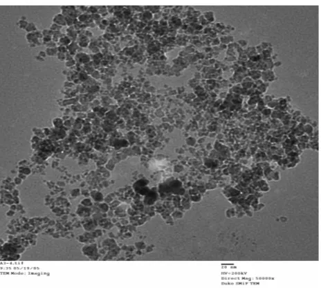
Using transmission electron microscopy, the average magnetite particle size was found to
Figure 5 TEM micrograph of magnetite particles in the MSG W11 ferrofluid
3 5
6
4
1 1 2
4 6
C
o
u
n
t
7.5 10 12.5 15 17.5 20 22.5
Figure 6 Distribution histogram of magnetite particle size in MSG W11 ferrofluid
Table 1 Magnetite Particle Diameter Mean and Std. Deviation
The nanoparticle diameters ranged from 7.5 nm to 22.5 nm.
Mean 13.5 nm
Std Dev 3.44 nm
A low and a high level loading of magnetite was selected, v/v 0.01 and v/v 0.10
respectively for the electrospinning solutions. Appendix A describes the calculations used
to determine the amount of ferrofluid needed to achieve the desired concentrations. The
calculations were based on the assumption that all of the water evaporates leaving only
PEO and magnetite in the resulting nanofiber.
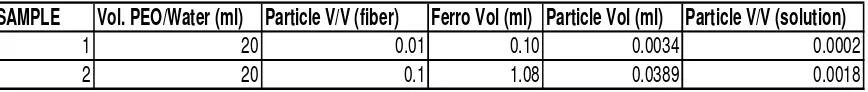
Table 2 Magnetite/ PEO volume fractions used in electrospinning trials
SAMPLE Vol. PEO/Water (ml) Particle V/V (fiber) Ferro Vol (ml) Particle Vol (ml) Particle V/V (solution)
1 20 0.01 0.10 0.0034 0.0002
2 20 0.1 1.08 0.0389 0.0018
3.1.2 VISCOSITY
An AR2000 rheometer (TA Instruments) was used to perform viscosity measurements of
the solutions. The concentric cylinder geometry was used to measure the stress and strain
profile of the pure PEO/water solution, electrospinning solutions, and the profile of the
pure ferrofluids. The Rheology Advance Instrument Control software was used to
0 500 1000 1500 2000 2500
V
is
c
o
s
it
y
(
c
P
)
1 10 100
Shear Rate (1/s)
Figure 7 AR2000 Viscosity profiles for PEO/water, 0.01 v/v magnetite/ PEO, 0.10 v/v magnetite/PEO, and pure MSG W11 ferrofluid
The viscosity of the PEO/water solution increased with increasing magnetite
concentration.
3.1.3 CONDUCTIVITY MEASUREMENTS
Conductivity Measurements were performed using a conductivity meter (Thermo) Orion
162A. 30ml aliquots of the PEO/water solution, PEO/magnetite (v/v 0.01), and
PEO/magnetite (v/v 0.10) were used for the conductivity measurements. The accuracy of
the meter is 0.5%.
Ferrofluid
PEO/Water
Magnetite/ PEO v/v 0.01
105.6 537.0 2050.0 0 500 1000 1500 2000 2500 C o n d u c ti v it y ( m ic ro S /c m )
0 0.01 0.1
Volume Fraction Magnetite Orion Conductivity Measurements
Figure 8 Conductivity Measurements for PEO/water, 0.01 v/v magnetite/ PEO, and 0.10 v/v magnetite/PEO
Figure 8 shows how increasing the loading of magnetite, increased the conductivity of the
electrospinning solutions.
3.1.4 SURFACE TENSION MEASUREMENTS
Surface tension measurements were performed using the Fisher Tensiomat Model 21. A
platinum-iridium ring was used. The force required to pull the ring out of the samples
was measured in dynes/cm. Normal laboratory temperature and humidity were used for
these measurements. Three repetitions of each measurement were performed and the
57.9
45.4
25.2
0.0 10.0 20.0 30.0 40.0 50.0 60.0
Surface Tension (dynes/cm)
PEO/Water PEO/Magnetite v/v
0.01
PEO/Magnetite v/v 0.10
Sample ID
Figure 9 Surface tension measurements for PEO/water, 0.01 v/v magnetite/ PEO, and 0.10 v/v magnetite/PEO
The inclusion of the magnetite particles produced a decrease in the PEO/water solution
surface tension.
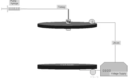
3.2 ELECTROSPINNING EXPERIMENTS
A parallel plate electrospinning apparatus was used to supply a uniform electric field for
the trials. Two aluminum plates with diameters of 12 inches were vertically aligned with
the distance between the two plates ranging from 15 cm- 25 cm. The solutions were
pumped at a specific flow rate using the NE 500 micro diaphragm pump by New Era
plastic syringe that was connected to the capillary tip using C-flex tubing with an inner
diameter of 0.125 inches. An electrical potential was applied using a Series EL DC High
Voltage power supply made by Glassman.
The plates were enclosed in a plastic enclosure. The bottom plate was positioned on an
adjustable lift that was used to set the plate to plate distance. The top plate had a 5 mm
hole in center of the plate to serve as the capillary tip entry point. The tip was aluminum
with an inner diameter of 0.75 mm and an outer diameter of 4 mm.
Figure 11 Schematic of NCSU laboratory parallel plate electrospinning set-up
3.3 MAGNETIC FIELD EXPERIMENTS
The magnetic field was supplied using an AC power supply connected to a solenoid of
magnetic wire. The solenoid had 30 turns of 13 gauge (1.8 mm diameter) copper magnet
wire. A Wavetek 2 MHz Sweep/Function Generator Model 19 was used to generate sine
wave functions. An AE Techron 5050 Linear Amplifier was used in conjunction with the
Wavetek Function Generator to supply alternating current. A glass capillary tip was used
with inner diameter of 1.5 mm. The solenoid was placed on the top plate and it
surrounded the glass capillary so that the magnetic field force would be downward
Figure 12 NCSU/UPRM laboratory electrospinning schematic with alternating magnetic field capabilities
3.4 ANALYSIS METHODS
3.4.1 SCANNING ELECTRON MICRCROSCOPY
A Hitachi SN 3200 variable pressure scanning electron microscope was used to retrieve
high resolution images of the fiber webs after electrospinning. The accelerating voltage
used varied from 0.3 kV- 30 kV with a working distance of 3-60 mm. The samples were
directly deposited on to aluminum foil during electrospinning. The fiber webs were
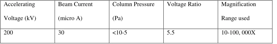
3.4.2 TRANSMISSION ELECTRON MICROSCOPY
A Hitachi HF-2000 Transmission Electron Microscope was used to analyze the fiber size
and particle distribution.
Figure 13 Duke University Shared Materials Instrumentation Facilities Hitachi HF-2000 TEM
The fibers were directly deposited onto 3 mm mesh copper TEM grids. The following
parameters were used as standard operating procedures.
Table 3 Hitachi HF-2000 Microscope settings
Accelerating
Voltage (kV)
Beam Current
(micro A)
Column Pressure
(Pa)
Voltage Ratio Magnification
Range used
200 30 <10-5 5.5 10-100, 000X
The HF-2000 is also equipped with a silicon x-ray detector for energy dispersive
spectroscopy. The analysis software used was INCA for elemental identification of the
3.4.3 SUPERCONDUCTING QUANTUM INTERFERENCE DEVICE
A superconducting quantum interference device (SQUID) was used to determine the
magnetic response of the fibers to an applied AC field. The Quantum Design
MPMS-XL7 SQUID magnetometer was used to determine the hysteresis behavior and the AC
out of phase component of the susceptibility of the fibers.
Figure 14 UPRM chemical engineering laboratory SQUID Magnetometer
Using the SQUID magnetometer, the susceptibility was measured as a function of the AC
4. RESULTS AND DISCUSSION
The values of the flow rate, applied voltage, plate to plate distance, and capillary tip size
were preliminarily screened to determine the operating parameters that would allow
whipping to occur. When whipping occurred PEO/magnetite fiber webs were formed
and collected on the bottom collector plate. Scanning electron microscopy was used to
examine the fibers.
Figure 15 SEM micrograph of magnetite/PEO electrospun fiber web containing 0.01 v/v magnetite particles
4.1 ELECTROSPINNING PHASE DIAGRAMS
Phase diagrams of three different solutions were developed: 2wt% PEO/water, PEO
solution with v/v 0.01 Fe3O4, and PEO solution with v/v 0.10 Fe3O4. The change in jet
flow was observed by lowering the laboratory lights and using a strobe lamp to illuminate
the electrospinning jet. The phase diagrams were completed to determine the electric
field and flow rate where dripping, stable flow, and whipping flow existed for each of the
three solutions. The electric field range was 0.4 kV/cm - 2 kV/cm and the flow rate range
tested was 0.1 ml/min to 0.3 ml/min.
0 0.5 1 1.5 2 2.5
0 0.05 0.1 0.15 0.2 0.25 0.3 0.35
Flowrate (ml/min)
E
F
ie
ld
(
k
V
/c
m
) Whipping
Stable Dripping
To transition from dripping to stable, an electric field of 1.25 kV/cm was required at all
flow rates. For pure PEO/water, the dripping and stable region were observed, but no
whipping phase was observed. Other researchers observed whipping phases in PEO/water
solutions; however, the solutions usually contained salts to increase the electrostatic
forces that promote whipping [9].
0 0.5 1 1.5 2 2.5
0 0.05 0.1 0.15 0.2 0.25 0.3 0.35
Flowrate (ml/min)
E
F
ie
ld
(
k
V
/c
m
)
Whipping Stable Dripping
Figure 17 Magnetite/ PEO (containing v/v 0.01magnetite) electrospinning phase diagram depicting the flow rate and electric field for dripping, stable, and whipping flow
For the PEO/water solution containing v/v 0.01 of magnetite, lower flow rates required a
higher field value to transition from dripping to stable than higher flow rates. In
comparison to pure PEO/water, the inclusion of the magnetite particles provided solution
Figure 18 illustrates a phase diagram for the PEO solutions containing v/v 0.10 of
magnetite. As with the v/v 0.01 solution, whipping occurred at field values between 1.6 -
1.8 kV/cm.
0 0.5 1 1.5 2 2.5
0 0.05 0.1 0.15 0.2 0.25 0.3 0.35
Flowrate (ml/min)
E
F
ie
ld
(
k
V
/c
m
) Whipping
Stable Dripping
Figure 18 Magnetite/ PEO (containing v/v 0.10 magnetite) electrospinning phase diagram depicting the flow rate and electric field for dripping, stable, and whipping flow
Several differences can be noted between the phase diagrams for the two solutions.
Lower applied fields were required to transition from dripping to stable for the solution
containing higher loads of magnetite. This difference may be attributed to the decrease in
surface tension. Lower surface tension implies a lower cohesiveness of the droplet;
therefore it is easier to transition from dripping to stable. Secondly, the shape of the
solution behaved more like solutions in the literature [9]. At higher flow rate, the fluid
carries less negative charge as it is headed toward the positive electrode; thereby
requiring higher field values at higher flow rates. The charge per unit volume is lower
with increasing flow rate; thereby higher fields are required for higher flow rates.
In evaluating the effects of the magnetite inclusion, it was shown that the magnetic
nanoparticles created solution properties favorable for whipping instability. The solution
containing higher loadings of magnetite had a higher conductivity, higher viscosity, and
lower surface tension. The magnetic particles lowered solution surface tensions and
increased conductivities to promote the transition from stable to whipping. . It was
observed that the whipping oscillations were more vigorous for the solution containing
more ferrofluid. The inclusion of the magnetite particles fashioned properties conducive
for nanofiber production.
4.2 FIBER CHARACTERIZATION
4.2.1 FIBER DIAMETER
Transmission electron microscopy was used to observe the fiber shape and size
distribution. Twenty fibers were measured to determine the average diameter size of the
fibers and the range of fiber sizes. Three measurements were taken of each fiber using
Image Tool software. The average diameter of the three measurements was plotted on a
50 100 150 200 M e a n F ib e r D ia m e te r (n m )
0 1 2 3 4 5 6 7 8 9 10 12 14 16 18 20 Fiber Number
Avg=86.85
Figure 19 X-bar chart of electrospun magnetite/ PEO ( containing v/v 0.01magnetite) average fiber diameter 150 200 250 300 350 400 450 500 550 M e a n F ib e r D ia m e te r (n m )
1 2 3 4 5 6 7 8 9 10 12 14 16 18 20 Fiber Number
Avg=275.08
Figure 20 X-bar chart of electrospun magnetite/ PEO ( containing v/v 0.10magnetite) average fiber diameter
The average diameter for the solutions having higher ferrofluids concentration (v/v 0.10)
was 275 nm in comparison to an average diameter of 87 nm for the lower concentration
solution. Including the variation in the diameter sizes, there was a statistical difference
between the two values. The higher magnetite loadings led to a larger fiber diameter.
both solutions. The difference exists in the solution parameters. The higher conductivity
solution and higher viscosity produced fibers with larger diameters. The solution surface
tension was lower, but the effect of the surface tension was outweighed by the effect of
the viscosity. Whipping occurred with an applied field of 1.8 kV in both cases, however
the higher loading solution produced fibers that were elongated less during the whipping
process.
Using transmission electron microscopy images of the PEO/magnetite fibers were
obtained. Fibers were deposited directly onto the TEM micrograph grids while whipping
occurred during the electrospinning process. Figures 21 and 22 are micrographs of PEO
Figure 22 TEM micrograph of PEO nanofiber containing 0.01 v/v magnetite nanoparticles
The dark regions in these fibers correspond to the magnetite nanoparticles dispersed
within the polyethylene oxide matrix. The micrographs show some particle
agglomeration within the fibers. The agglomeration could be attributed to the mixing
process during the preparation of the spinning solutions, or settling of the particles from
Figure 24 TEM micrograph of PEO nanofiber containing 0.10 v/v magnetite nanoparticles
Figures 23 and 24 are micrographs of the fibers containing 0.10 v/v magnetite particles.
From these micrographs it can be seen that the fibers containing larger magnetite loading
were concentrated with nanoparticles in comparison to the randomly dispersed particles
seen in the lower concentration fibers.
4.2.2 ENERGY DISPERSIVE SPECTROSCOPY
Energy dispersive spectroscopy was used to identify the elements present in the fibers
analyzed. The characteristic x-rays for iron, carbon, and oxygen were identified in all
samples. This quantitative analysis showed an increase in the relative intensities of the
Figure 25 EDS spectrograph for PEO nanofiber containing 0. 01 v/v magnetite nanoparticles
Table 4 EDS summary for PEO nanofiber containing 0. 01 v/v magnetite nanoparticles
Element Weight %
Carbon 94.4
Iron 5.6
Table 5 EDS summary for PEO nanofiber containing 0. 10 v/v magnetite nanoparticles
Element Weight %
Carbon 15.7
Oxygen 25.5
Iron 58.8
The iron alpha peak was identified in all samples at 6. 40 keV, the higher energy
K-beta peak was found at 7.06 keV. The iron L-series peaks were not resolved into
individual peaks, but combined into one peak at 0.71 keV. The K- alpha peak of oxygen
was identified at 0.52 keV. K and L denote the shells from which the electrons were
removed. Alpha transitions occur when an electron moves from L shell to the K shell;
beta transitions occur when an electron moves from the M shell to the K shell.
Oxygen is present in the polyethylene oxide matrix but also in the magnetite crystal
structure. At higher magnetite levels, the oxygen produced a more prominent and intense
spectra. Carbon’s K-alpha peak at 0.28 keV was found in both samples.
The weight percent of iron in the samples increased from 5.6% for v/v 0.01 of magnetite
fiber to 58.83 % for v/v 0.10 magnetite fibers. In Appendix A, calculations are shown
that determine the weight percent magnetite in the final fiber. The calculations predicted
that polyethylene nanofibers containing v/v 0.01 magnetite would have 4.5 wt%
magnetite. This designed value is similar to the 5.6% predicted by EDS. Also it was
calculated that the polyethylene nanofibers containing v/v 0.10 magnetite particles would
have 45.6 wt% magnetite. The differences in the EDS estimated value and the calculated
values reside in the fact that EDS must be calibrated using a standard to exactly quantify
During analysis of the 0.10 v/v magnetite fiber, the existence of a sulfur k-alpha peak
was identified. This peak was attributed to the surfactant layer of the ferrofluids. The
copper peak identified is due to the copper grid that the fibers were deposited on for TEM
analysis.
4.3 MAGNETIC CHARACTERIZATION
4.3.1 SQUID HYSTERESIS
The hysteresis curve revealed the magnetic properties of the fibers. The saturation point,
Ms, the amount of magnetization retained, Mr, and the coercivity Hc of the fibers are all
-0.025 -0.02 -0.015 -0.01 -0.005 0 0.005 0.01 0.015 0.02 0.025
-6.00E+04 -4.00E+04 -2.00E+04 0.00E+00 2.00E+04 4.00E+04 6.00E+04
H (Oe)
M
(
e
m
u
)
Ms
Mr
Hc
-20 -15 -10 -5 0 5 10 15 20
-6.00E+04 -4.00E+04 -2.00E+04 0.00E+00 2.00E+04 4.00E+04 6.00E+04
H (Oe)
M
(
e
m
u
/g
)
Ms
Mr
Hc
Figure 28 Room temperature hysteresis curve for electrospun PEO nanofiber containing 0.10 v/v magnetite nanoparticles
In Figures 27 and 28, it can be observed that the saturation magnetization increases with
increasing magnetite concentration. This is due to the fact that those fibers contained
more domains to contribute to the magnetic flux. The TEM micrographs of the fibers
with the lower concentration of ferrofluids showed clustering of particles. The clusters of
particles act to cancel out the magnetic moments of the surrounding particles; thereby
reducing the contribution of the particles to the magnetic flux.
The remnant magnetization of the lower concentration fiber was 0.0241 emu/g in
comparison to 0.0811 emu/g for the higher loading fiber sample. The remnant
after the applied field was removed, more domains remained aligned in the fiber
containing the higher concentration magnetite.
4.3.2 SQUID AC SUCEPTIBILITY
Figure 29 shows the out-of-phase component of the AC susceptibility for the two
samples of fibers.
0 0.000005 0.00001 0.000015 0.00002 0.000025
0 200 400 600 800 1000 1200
Wave Frequency (Hz)
C
h
i'
'/
d
V/V 0.01 V/V 0.10
0 0.000005 0.00001 0.000015 0.00002 0.000025
0 20 40 60 80 100 120 140 160 180 200
Wave Frequency (Hz)
C
h
i'
'/
d V/V 0.01
V/V 0.10
Figure 30 Out-of-phase component of the AC susceptibility for PEO nanofibers containing v/v 0.01 and v/v 0.10 magnetite nanoparticles
The two fiber samples tested had basically identical spectra pattern.
Distinct peaks were seen in both fibers at 30 Hz, 40 Hz, and 110 Hz. These distinct
4.4 ALTERNATING MAGNETIC FIELD
Experiments were performed to combine an alternating magnetic field with the parallel
plate electrospinning set-up. Initially the solenoid was placed on the top plate of the
electrospinning apparatus as shown in Figure 31. Prior to beginning electrospinning, an
amplitude value of 3-4 amps was supplied to the solenoid to create the alternating
magnetic field with a frequency of 1 kHz.
Figure 31 Electrospinning set-up #1 with AC magnetic field capabilities
Using a gauss meter, a magnetic field force of ~21 Gauss was measured at Point 1 on the
solenoid, but a force of only 0.3 Gauss was detected at the tip exit located on the
underside of the top plate. Aluminum is nonmagnetic, and its relative magnetic
permeability is approximately 1, therefore it is as permeable as air. The aluminum
permeability is such that it should not prevent the field from permeating to Point 2. It
was concluded that the distance from the solenoid to the tip exit was beyond the range of
Next a 30 gauge copper wire was used that would allow the solenoid to go through the
top plate aperture, as shown in Figure 32. The solenoid extended to the exit of the tip.
Figure 32 Electrospinning set-up #2 with AC magnetic field capabilities
This set-up allowed the field force to be perpetuated onto both sides of the solenoid
equally with a value of 21 Gauss. The amplitude of the current caused the wire to begin
to burn and disintegrate. It was discovered that the higher gauge wire could not support
the desired AC current amplitude.
Finally to supply the alternating magnetic field, the solenoid was placed between the two
Figure 33 Electrospinning set-up #3 with AC magnetic field capabilities
The set-up shown in Figure 33 allowed for the use of the original lower gauge magnet
wire capable of withstanding the desired current amplitude. The combination of the
magnetic field and the electrospinning voltage created arcing. Arcing occurs when an
electrical current discharge moves from one electrode to another. This prevented the
experiment form continuing without damaging the equipment. By switching the positive
and negative electrodes on the plates, arcing was avoided; however this led to
electrospinning to occur from the bottom up as demonstrated in Figure 33. The
Figure 34 Backward Electrospinning Schematic
create an attraction to the top plate. The fibers flowing from bottom up, interfered with
5 CONCLUSIONS
Nanocomposite polyethylene oxide (PEO) fibers containing individual magnetic domains
were spun using parallel plate electrospinning. The fibers were spun from solutions dosed
with nanoparticles of magnetite (Fe3O4) at various loading fractions in 2 wt% PEO in
water. A high (v/v 0.10) and a low (v/v 0.01) magnetite dosed solution were used to
determine how the processing parameters and fiber properties changed as a function of
nanoparticle concentration.
The inclusion of the magnetic nanoparticles produced solutions with higher conductivity,
lower surface tension, and higher viscosity. Phase diagrams were constructed to show
the three regions: dripping, stable, and whipping. Higher viscosity solutions were spun
without significantly higher electric field requirements due to the reduction in surface
tension and higher conductivity.
Electrospinning was used to produce fibers with diameters as low as 45 nanometers.
Transmission electron microscopy showed that the average fiber diameter increased with
increasing magnetite concentration. Energy dispersive spectroscopy showed an increase
in iron characteristic x-rays for the higher loading fiber samples. The saturation and
remnant magnetization was higher for v/v 0.10 fibers due to the contribution of the
domain alignment. Unique AC susceptibility signatures were identified using SQUID
6 SUGGESTIONS FOR FURTHER RESEARCH
Many possibilities exist for future work in the area of electrospinning nanofibers.
Currently energy requirements for the electrospinning process limit its feasibility as a full
scale production process. This work identified new avenues that future researchers can
use to lower the energy requirements.
The first suggestion involves analyzing the effect of the capillary tip. Two tips were used
during this research: a aluminum tip (i.d.0.75 mm) and a glass tip (i.d.1.5 mm). The
difference between the two reside in the materials of construction and the tip size. Phase
diagrams were constructed using the glass capillary tip and the applied voltage to achieve
stable and whipping flow was dramatically reduced compared to the energy requirements
Phase Diagram Commercial Ferrofluid 2wt% PEO Water
0.10 Vol Fraction Ferro Glass Capillary 0.3 0.4 0.5 0.6 0.7 0.8 0.9 1
11.5 12 12.5 13 13.5 14 14.5
Flowrate (ml//hr) E F ie ld ( k V /c m ) Whipping Stable Dripping
Figure 35 Magnetite/ PEO (containing v/v 0.10 magnetite) electrospinning phase diagram depicting the flow rate and electric field for dripping, stable, and whipping flow using glass tip
For identical processing parameters, 19 kV and 45 kV were required for whipping with
the glass and aluminum capillaries respectively. This reduction is attributed to the ease at
which the charge was able to contact the solution with the glass tip. The walls of the
glass tip were 0.3 mm compared to ~ 3mm for the aluminum tip. Future investigation is
suggested to explore the impact of the effect of tip size and material of construction.
The negative viscosity effect theoretically supplies a way to alter solution viscosity, the
most important factor in determining final fiber diameter. Modifications to the
(a) A top plate with larger aperture that can accommodate a solenoid of magnetic
wire insulated by a dielectric material to prevent arcing
Figure 36 Recommended solenoid enclosed in dielectric material for electrospinning with AC magnetic field
(b) Electrically connect the solenoid to the electrospinning plates to prevent arcing
Either suggestion (a) or (b) could allow for the incorporation of the alternating magnetic
field into the electrospinning set-up.
Finally, particle agglomeration occurred in samples with lower concentration of
magnetite. Functionalizing the particles with a layer of PEO could improve the dispersion
of the particles within the polymer solutions. The University of Puerto Rico at Mayaguez
synthesized thiolated nanoparticles with PEO. Below is a micrograph of v/v 0.01 loading
Figure 37 TEM micrograph of PEO nanofiber containing 0.01 v/v functionalized magnetite nanoparticles
This functionalization greatly improved the particle dispersion within the fiber matrix and
7 REFERENCES
1. Lubbe, A.S., C. Alexiou, and C. Bergemann, Clinical applications of magnetic drug targeting. Journal of Surgical Research, 2001. 95(2): p. 200-206.
2. Wilson, J.L., et al., Synthesis and magnetic properties of polymer nanocomposites with embedded iron nanoparticles. Journal of Applied Physics, 2004. 95(3): p.
1439-1443.
3. Verma, S. and P.A. Joy, Magnetic properties of superparamagnetic lithium ferrite nanoparticles. Journal of Applied Physics, 2005. 98(12).
4. Marchessault, R.H., P. Rioux, and L. Raymond, Magnetic Cellulose Fibers and Paper - Preparation, Processing and Properties. Polymer, 1992. 33(19): p.
4024-4028.
5. Huang, Z.M., et al., A review on polymer nanofibers by electrospinning and their applications in nanocomposites. Composites Science and Technology, 2003.
63(15): p. 2223-2253.
6. Spivak, A.F., Y.A. Dzenis, and D.H. Reneker, A model of steady state jet in the electrospinning process. Mechanics Research Communications, 2000. 27(1): p.
37-42.
7. Li, D. and Y.N. Xia, Electrospinning of nanofibers: Reinventing the wheel?
Advanced Materials, 2004. 16(14): p. 1151-1170.
8. Theron, S.A., E. Zussman, and A.L. Yarin, Experimental investigation of the governing parameters in the electrospinning of polymer solutions. Polymer, 2004.
45(6): p. 2017-2030.
9. Hohman, M.M., et al., Electrospinning and electrically forced jets. II. Applications. Physics of Fluids, 2001. 13(8): p. 2221-2236.
11. Li, D., T. Herricks, and Y.N. Xia, Magnetic nanofibers of nickel ferrite prepared by electrospinning. Applied Physics Letters, 2003. 83(22): p. 4586-4588.
12. Demir, M.M., et al., Electrospinning of polyurethane fibers. Polymer, 2002.
43(11): p. 3303-3309.
13. Duan, B., et al., Electrospinning of chitosan solutions in acetic acid with poly(ethylene oxide). Journal of Biomaterials Science-Polymer Edition, 2004.
15(6): p. 797-811.
14. Mit-uppatham, C., M. Nithitanakul, and P. Supaphol, Ultratine electrospun polyamide-6 fibers: Effect of solution conditions on morphology and average fiber diameter. Macromolecular Chemistry and Physics, 2004. 205(17): p.
2327-2338.
15. Reneker, D.H. and I. Chun, Nanometre diameter fibres of polymer, produced by electrospinning. Nanotechnology, 1996. 7(3): p. 216-223.
16. Zhao, Y.Y., et al., Study on correlation of morphology of electrospun products of polyacrylamide with ultrahigh molecular weight. Journal of Polymer Science Part B-Polymer Physics, 2005. 43(16): p. 2190-2195.
17. Zhao, Z.Z., et al., Preparation and properties of electrospun poly(vinylidene fluoride) membranes. Journal of Applied Polymer Science, 2005. 97(2): p.
466-474.
18. Ristolainen, N., et al., Poly(vinyl alcohol) and polyamide-66 nanocomposites prepared by electrospinning. Macromolecular Materials and Engineering, 2006.
291(2): p. 114-122.
19. Gupta, P., et al., Electrospinning of linear homopolymers of poly(methyl methacrylate): exploring relationships between fiber formation, viscosity,
molecular weight and concentration in a good solvent. Polymer, 2005. 46(13): p.
4799-4810.
20. Pornsopone, V., et al., Electrospinning of methacrylate-based copolymers: Effects of solution concentration and applied electrical potential on morphological appearance of as-spun fibers. Polymer Engineering and Science, 2005. 45(8): p.