Gene Subset Selection Approaches Based on Linear Separability

(1)

Scholarship at UWindsor

Electronic Theses and Dissertations Theses, Dissertations, and Major Papers

2011

Gene Subset Selection Approaches Based on Linear Separability

Amirali Jafarian

University of Windsor

Follow this and additional works at: https://scholar.uwindsor.ca/etd

Recommended Citation Recommended Citation

Jafarian, Amirali, "Gene Subset Selection Approaches Based on Linear Separability" (2011). Electronic Theses and Dissertations. 7908.

https://scholar.uwindsor.ca/etd/7908

(2)

by

Amirali Jafarian

A Thesis

Submitted to the Faculty of Graduate Studies

through Computer Science

in Partial Fulfillment of the Requirements for

the Degree of Master of Science at the

University of Windsor

Windsor, Ontario, Canada

2011

(3)

**1*1**

Published Heritage Branch

395 Wellington Street OttawaONK1A0N4 Canada

Direction du

Patrimoine de I'edition

395, rue Wellington OttawaONK1A0N4 Canada

Your file Votre reference ISBN: 978-0-494-81742-1 Our file Notre r6f6rence ISBN: 978-0-494-81742-1

NOTICE: AVIS:

The author has granted a

non-exclusive license allowing Library and Archives Canada to reproduce, publish, archive, preserve, conserve, communicate to the public by

telecommunication or on the Internet, loan, distribute and sell theses

worldwide, for commercial or non-commercial purposes, in microform, paper, electronic and/or any other formats.

L'auteur a accorde une licence non exclusive permettant a la Bibliotheque et Archives Canada de reproduire, publier, archiver, sauvegarder, conserver, transmettre au public par telecommunication ou par I'lnternet, preter, distribuer et vendre des theses partout dans le monde, a des fins commerciales ou autres, sur support microforme, papier, electronique et/ou autres formats.

The author retains copyright ownership and moral rights in this thesis. Neither the thesis nor substantial extracts from it may be printed or otherwise reproduced without the author's permission.

L'auteur conserve la propriete du droit d'auteur et des droits moraux qui protege cette these. Ni la these ni des extraits substantiels de celle-ci ne doivent etre imprimes ou autrement

reproduits sans son autorisation.

In compliance with the Canadian Privacy Act some supporting forms may have been removed from this thesis.

Conformement a la loi canadienne sur la protection de la vie privee, quelques

formulaires secondaires ont ete enleves de cette these.

While these forms may be included in the document page count, their removal does not represent any loss of content from the thesis.

Bien que ces formulaires aient inclus dans la pagination, il n'y aura aucun contenu manquant.

1+1

(4)

I. Co-Authorship Declaration

I hereby declare that this thesis incorporates material that is result of joint research, as

follows:

This thesis also incorporates the outcome of a joint research undertaken in collaboration

under the supervision of Professor Dr. Alioune Ngom. The collaboration is covered in

Chapter 3 and 4 of the thesis. In all cases, the key ideas, primary contributions,

experimental designs, data analysis and interpretation, were performed by the author, and

the contribution of co-authors was primarily through the provision of advice when

needed.

I am aware of the University of Windsor Senate Policy on Authorship and I

certify that I have properly acknowledged the contribution of other researchers to my

thesis, and have obtained written permission from each of the co-authors to include the

above materials in my thesis.

I certify that, with the above qualification, this thesis, and the research to which it

refers, is the product of my own work.

II. Declaration of Previous Publication

This thesis includes 3 original papers that have been previously published/submitted for

publication in peer reviewed conferences, as follows:

(5)

3 and 4

A New Gene Subset Selection Approach Based on Linear Separating Gene Pairs, IEEE International Conference on Computational Advances in Bio and medical Sciences (ICCABS 2011), Orlando FL, Feb 3-5, 2011,pp.l05-110.

A Novel Recursive Feature Subset Selection Algorithm, 11th IEEE International Conference on Bioinformatics & Bioengineering, Taichung, Taiwan, October 24-26 2011

New Gene Subset Selection Approaches Based on Linearly Separating Genes and Gene-Pairs, the 6th International Conference on Pattern recognition in Bioinformatics, Delft, Netherlands, November 2-4 2011

published

submitted

1 certify that I have obtained a written permission from the copyright owners to

include the above published materials in my thesis. I certify that the above material

describes work completed during my registration as graduate student at the University of

Windsor.

1 declare that, to the best of my knowledge, my thesis does not infringe upon

anyone's copyright nor violate any proprietary rights and that any ideas, techniques,

quotations, or any other material from the work of other people included in my thesis,

published or otherwise, are fully acknowledged in accordance with the standard

referencing practices. Furthermore, to the extent that I have included copyrighted

(6)

owners to include such materials in my thesis.

1 declare that this is a true copy of my thesis, including any final revisions, as

approved by my thesis committee and the Graduate Studies office, and that this thesis has

not been submitted for a higher degree to any other University or Institution.

(7)

We address the concept of linear separability of gene expression data sets with

respect to two classes, which has been recently studied in the literature. The problem is to

efficiently find all pairs of genes which induce a linear separation of the data. We study

the Containment Angle (CA) defined on the unit circle for a linearly separating gene-pair

(LS-pair) as an alternative to the paired t-test ranking function for gene selection. Using

the CA we also show empirically that a given classifier's error is related to the degree of

linear separability of a given data set. Finally we propose gene subset selection methods

based on the CA ranking function for LS-pairs and a ranking function for linearly

separation genes (LS-genes), and which select only among LS-genes and LS-pairs.

Overall, our proposed methods give better results in terms of subset sizes and

classification accuracy when compared to well-performing methods, on many gene

(8)

To my beloved mother

for all your love, support and faith

I love you

(9)

First of all, I would like to convey my sincere gratitude to my supervisor, Dr.

Alioune Ngom for his excellent supervision, advice and guidance throughout this thesis.

Without his help and guidance this thesis would not have been completed. Also, he

provided me unflinching encouragement and support in various ways.

Besides, I would also like to thank my internal reader, Dr. Luis Rueda, who has

contributed in our research and gave us precious ideas to improve the quality of this

research. Also, I would like to thank members of my master committee, Dr. Kemal Tepe,

Department of Electrical and Computer Engineering, Dr. Luis Rueda, School of

Computer Science, and Dr. Jianguo Lu, the chair of the committee for their constructive

(10)

DECLARATION OF CO-AUTHORSHIO AND PREVIOUS PUBLICATION iii

ABSTRACT vi

DEDICATION vii

ACKNOWLEDGEMENTS viii

LIST OF TABLES xii

LIST OF FIGURES xv

CHAPTER

I. INTRODUCTION

1. Problem Statement 3

2. Outline 5

II. REVIEW OF LITERATURE

1. Filter Methods 6 1.1. Univariate methods 7

\.\.\.t-test 7

1.1.2. Fisher Criterion 8 1.1.3. Signal to noise statistics 8

1.1.4.x2 Statistics 8 1.1.5. Relief Algorithm 9 1.1.6.T-NOM 10 1.2. Multivariate methods 10

1.2.1. Minimum Redundancy and Maximum Relevancy

(mRMR) 11 1.2.2. Pair based method based with /-test [2] 12

2. Wrapper Methods 12 2.1. Forward Selection and Backward Selections 13

2.2. Floating Search 14 2.3. TAFS Algorithm 15 3. Embedded methods 15

3.1. SVM-RFE 16 4. Linearly Separability of Gene Expression Datasets 16

4.1. Algorithm of Linear Separability [1]: 20

(11)

Separating Genes and Pairs of Genes 21

1.1. LS-Pair Ranking Criterion 21 1.2. LS-Genes Ranking Criterion 25 1.3. Search strategies for selecting LS genes and LS pairs.25

1.3.1.LS Approach 27 1.3.2. LSGP Approach 28 1.3.3. Graph-Based Methods 29 2. Recursive Feature Subset selection 33

2.1. LS samples vs. non-LS samples 35 2.2. Recursive Feature Selection Algorithm 36

2.2.1. Ranking criteria 38

IV. COMPUTATIONAL EXPERIMENTS

1. Comparison of the pair based algorithms with the

greedy pair method of [2] 39 2. Comparison of the pair based algorithm with mRMR [6]43

3. Comparison between our pair based approaches 46

4. Comparison of the Recursive Algorithm with baselines

and mRMR [6] 47 5. Train and Test Procedure 50

5.1. Reporting a single subset of genes 54

5.1.1. Frequent Genes Reporting 54 5.1.2. Best Subset Report 58

6. Summary 62 7. Comparison of running time 63

V. DATASETS AND MATERIALS

1. Datasets 65 2. Pre-Processing Steps 65

VI. CONCLUSIONS AND FUTURE W O R K

1. Conclusion and Discussion 68

2. Future Work 69

APPENDICES

Gene Report 70

(12)

(13)

TABLE 1. DEGREE OF SEPARABILITY OF DATASETS 19

TABLE 2. AVERAGE OF CLASSIFIERS' PERFORANCES ON BOTTOM 10 (B) AND TOP 10 (T) LS

PAIRS 23

ON BEST-S'S

46

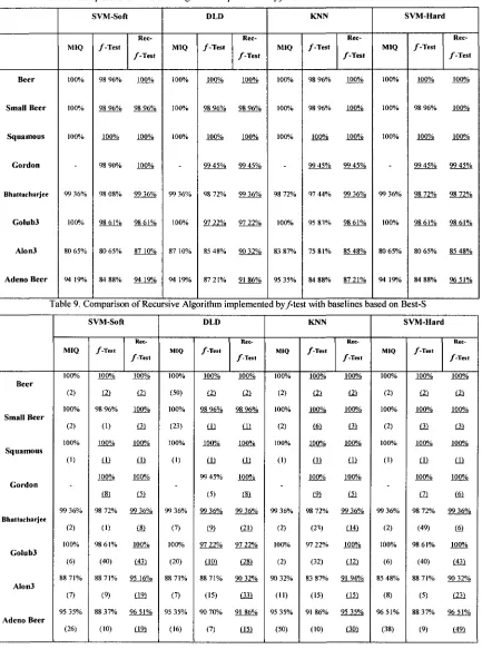
TABLE 8. COMPARISON OF RECURSIVE ALGORITHM IMPLEMENTED BY F-TEST WITH

BASELINES BASED ON SUBSETS S 48

TABLE 9. COMPARISON OF RECURSIVE ALGORITHM IMPLEMENTED BY F-TEST WITH

BASELINES BASED ON BEST-S 48

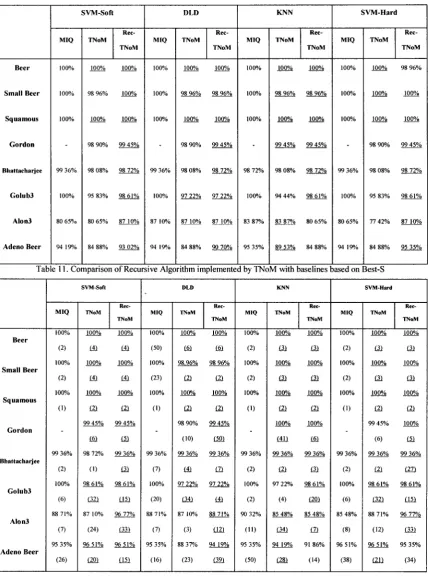
TABLE 10. COMPARISON OF RECURSIVE ALGORITHM IMPLEMENTED BY T N O M WITH

BASELINES BASED ON SUBSETS S 49

TABLE 11. COMPARISON OF RECURSIVE ALGORITHM IMPLEMENTED BY T N O M WITH

BASELINES BASED ON BEST-S 49

TABLE

12.

ACCURACY OF

S

FOR

[XX]-LSGP,

WITH RANKING AND SELECTION ON TRAINPWG

SETS 51

TABLE

13.

ACCURACY OF BEST-S FOR

[XX]-LSGP,

WITH RANKING AND SELECTION ON

(14)

BASELINES, WITH RANKING AND SELECTION ON TRAINING SETS 53

TABLE

23 BF-LSGP

APPROACH

60

TABLE 24PERFORMANCE OF THE BEST SUBSETS OF GENES WITH F-TEST VS. REC- F-TEST..60

TABLE 25 PERFORMANCE OF THE BEST SUBSETS OF GENES WITH T N O M VS REC-TNOM...61

TABLE 26. SUMMARY OF ATTRIBUTES OF ALGORITHMS 62

TABLE 27. SUMMARY OF THE BEST ACCURACIES ACHIEVED WITH DIFFERENT INTRODUCED

APPROACHES 63

TABLE 28. COMPARISON OF RUNNING TIMES OF PAIR SELECTION AND THE RECURSIVE

LAGORITHM 6 4

APPROACH 76

TABLE 37. TOP 50 BEST GENES WITH SVM-SOFT FOR ALON DATASET USING REC-TNOM

(16)

FIGURE 1. AN LS PAIR TAKEN FROM GOLUB (LEUKEMIA) DATASET 17

FIGURE 2. ANON-LS PAIR TAKEN FROM GOLUB (LEUKEMIA) DATASET 17

FIGURE 3. A SET OF FOUR NON-SEPARABLE POINTS, (A) THE CONSTRUCTION OF THE

VECTORS, (B) THEIR PROJECTION ONTO THE UNIT CIRCLE [1] 18

FIGURE 4. A SET OF FOUR SEPARABLE POINTS PRODUCING VECTORS ON THE UNIT CIRCLE

THAT ARE CONTAINED IN A SECTOR OF ANGLE B < 180° [1] 18

FIGURE 5. A SET OF POINTS CAUSING LINEAR SEPARABILITY (LEFT PANEL) VS. NON

LPWEAR SEPARABILITY (RIGHT PANEL) 25

FIGURE 6. THE PROJECTION OF VECTORS OF LS POINTS IN THE ZERO-SPHERE (LEFT PANEL)

Vs. NON LINEAR SEPARABILITY (RIGHT PANEL) 25

FIGURE 7. RANKING CRITERION FOR LS GENES 25

FIGURE 8. EXAMPLES OF LS-SAMPLES VS. NON-LS SAMPLES 34

FIG 9. PERFORMANCE OF SVM-HARD ON GOLUB2 41

FIGURE 10. PERFORMANCE OF SVM-SOFT ON GOLUB2 41

FIGURE 11. PERFORMANCE OF KNN ON GOLUB2 41

FIGURE 12. PERFORMANCE OF DLD ON GOLUB2 41

FIGURE 13. PERFORMANCE OF QDA ON GOLUB2 41

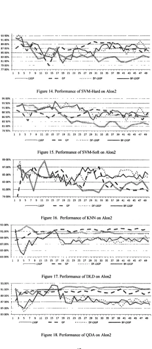
FIGURE 14. PERFORMANCE OF SVM-HARD ON ALON2 42

FIGURE 15. PERFORMANCE OF SVM-SOFT ON ALON2 42

FIGURE 16. PERFORMANCE OF KNN ON ALON2 42

FIGURE 17. PERFORMANCE OF DLD ON ALON2 42

(17)

(18)

INTRODUCTION

DNA microarrays give the expression levels for thousands of genes in parallel either for a

single tissue, condition, or time point. In the former the snapshot of the expression of

genes for different samples is taken, whereas the latter shows the expression for a period

of time. Microarray data sets are also usually noisy with a low sample size given the large

number of measured genes. Such data sets present many difficult challenges for sample

classification algorithms. Since many genes are irrelevant to the target classes,

considering them would not only introduce noise and degrade the classification

performance, but also increase the computational time. Furthermore, with this huge

number of genes, we have the problem of curse of dimensionality and the classification

algorithms trained upon the data would be prone to the problem of over-fitting. The small

number of samples makes it even worse. Hence in order to avoid the problems of

over-fitting and curse of dimensionality, feature selection algorithms are applied to reduce the

dimension of data to have at least faster and satisfactory classification accuracy with far

less numbers of features selected. In addition, with filtering irrelevant genes, the

biological information which was already hidden will be manifested. The feature subset

selection problem is to find a smallest subset of genes, whose expression values allow

sample classification with the highest possible accuracy; however Chen et al. [17]

showed that finding the smallest feature subset selection is an NP-hard problem and some

heuristic algorithms are needed to search for the optimal subset of genes. Feature subset

selection methods have received considerable attention in recent years as better

(19)

dimensionality reduction methods than feature extraction methods, which yield features

that are difficult to interpret. Many approaches have been proposed in the literature to

solve this problem. A simple and common method is the filter approach, which first

ranks single genes according to how well they each separate the classes and then selects

the top r ranked genes as the gene subset to be used; where r is the smallest integer,

which yields the best classification accuracy when using the subset. Also many feature

ranking criteria are proposed based on different (or a combination of) principles,

including redundancy and relevancy [2], [6]. Filter methods are simple and fast, but they

do not necessarily produce the best gene subsets. Filter methods often deal with each

gene separately and when each gene is considered individually, features' dependencies

may be ignored, which may lead to unsatisfactory classification performance. Hence, in

order to overcome this problem, a few multivariate filter techniques and wrapper

methods have been introduced; multivariate filtering approaches can distinguish the

target function better and model features' dependencies. Other methods introduced in

literature are the wrapper approaches, which evaluate subsets of genes irrespective of

any possible ranking over the genes. Such methods are based on heuristics which directly

search the space of gene subsets and are guided by a classifier's performance on the

selected gene subsets [9]. The best methods combine both gene ranking and wrapper

approaches but they are computationally intensive.

Beside gene subset selection, in the context of microarray data many other analyses

have been intensively studied, one of which is clustering; the problem in clustering is to

find genes, which share similar patterns; the motivation of finding these genes is that they

(20)

1. Problem Statement

As already mentioned better approaches in filter methods are multivariate methods,

modeling features' dependencies. However there are still only a few works for

multivariate filtering approaches (eg., Selection of pairs of genes, triplets of genes or

even group of genes) and most of the filtering approaches are categorized as univariate

filtering approaches, where genes are ranked separately and the dependencies are

ignored; therefore we believe gene subset selection, more specifically multivariate

filtering approaches deserve more consideration.

In this thesis first we present gene subset selection methods based on the concept of

linear separability of gene expression data sets as introduced recently in [1]. We use their

geometric notion oi linear separation by pairs of genes (where samples belong to one of

two distinct classes termed red and blue samples in [1]) to define a simple criterion for

selecting (best subsets of) genes for the purpose of sample classification. It has been

suggested that an underlying molecular mechanism relates together the two genes of a

separating pair to the phenotype under study, such as a specific cancer. Recently, some

authors have considered pairs of genes as features to be used in filtering methods rather

using than single genes. The motivation for using gene-pairs instead of single genes is

that two single genes considered together may distinguish the classes much better than

when they are considered individually; this is true even if one or both of the genes have

low ranks from a ranking function defined for single genes. In other words, when we

select only top-ranked single genes using such ranking function, some subsets of genes,

which have greater class distinguishing capability (than the subset of top-ranked genes),

(21)

will not be selected due to the presence of low-ranked single genes. The authors of [2]

devised the first gene selection method based on using pairs of genes as features. Given a

gene-pair, they used diagonal linear discriminant (DLD) and compute the projected

coordinate of each sample data on the DLD axis using only the two genes, and then take

the two-sample ^-statistic on these projected samples as the pair's score. The authors then

devised two filter methods for gene subset selection based on the pair ^-scores. Our

approach in this thesis is to use both linearly separating single genes (LS-genes) and

linearly separating gene-pairs (LS-pairs) as features for the purpose of finding the best

gene subsets. We propose ranking criteria for both LS-genes and LS-pairs in order to

evaluate how well such features separate the classes then devise methods that select

among top-ranked LS-genes and LS-pairs.

Also as already mentioned univariate filter methods, which rank single genes

according to how well they each separate the classes, are widely used for gene ranking in

the field of microarray analysis of gene expression datasets. These methods rank all of

the genes by considering all of the samples; however some of these samples may never

be classified correctly by adding new genes and these methods keep adding redundant

genes covering only some parts of the space and finally the returned subset of genes may

never cover the space perfectly. In this thesis we also introduce a new gene subset

selection approach which aims to add genes covering the space which has not been

(22)

2. Outline

The rest of this document is organized as follows. Chapter 2 provides a literature review

in the field of gene selection approaches. The fundamental part of this document is

chapter 3, where our approaches for gene subset selection are described. Chapter 4

discusses the computational results obtained with our approaches and different

experiments conducted to test the performance of our proposed approaches. Chapter 5

presents the details of datasets and pre-processing steps used in this thesis. Finally in

chapter 6 we conclude and cite some possibilities for future works.

(23)

REVIEW OF LITERATURE

The main aim of this chapter is to provide the reader with a literature review of the

previous important works done in the field of gene selection. Currently three major types

of feature selection techniques, depending on how the feature selection search combines

with the construction of the classification model, have been intensively employed in the

field of gene selection and dimension reduction in microarray datasets. They are filter

methods, wrappers methods, and embedded methods [18]. The three first sections of this

chapter are categorized based on these three types of gene selection techniques

mentioned, while the last part gives an overview of the recent work of Unger and Chor

[1], who introduced the concept of linear separability of gene expression datasets.

1. Filter Methods

Filter methods attempt to select features based on intrinsic nature of the data. In these

methods the gene selection process and classification process are separated; that is, first

features' scores are calculated and then low-scoring features are filtered out, finally the

remaining top ranked features will be used as input to machine learning classification

algorithms. This kind of selection is faster, simpler and the selected genes give better

generalization to unseen samples' classification [12]. Filter methods often treat mostly

each gene separately and when each gene is considered individually, features'

(24)

performance [12]. Hence, in order to cope with this problem, a number of multivariate

filter techniques and wrapper methods have been introduced; in the latter one (discussed

in section 2 of this chapter) gene selection is directed by a classifier's performance in

order to obtain the optimal subset of gene [9]. In this section, we discuss some univariate

filter methods, followed by multivariate filter methods.

1.1. Univariate methods

As already mentioned univariate methods consider each gene separately and due to high

dimension of microarray datasets, fast univariate techniques of filter methods have

attracted the attention of many researchers.

1.1.1. t-test

One of the most used statistical filter methods is t-test. For a dataset 5* consisting of n

features and m samples, the label of which is either +1 or -1 (2 class problem), the t-test

criterion is calculated by the eq.l, in which for each gene the mean [i* (resp., jutr) and the

standard deviation a* (resp., oj~) of samples of positive class (resp., negative class) are

used [22].

T(xi)-.

W

-^ (Eq.l)

-J

n+ n

-Also, in the eq.l, n+ (resp., «-) is the number of samples labeled as +1 (resp., -1).

(25)

1.1.2. Fisher Criterion

Similarly, Fisher's criterion [26] evaluates the degree of separation between two classes,

being defined as follows:

Jigd = H^r (

Ec

i-

2 )

ai +al

Hedenfalk et al. [26] used /-test and Fisher Criteria in gene expression profiles of

breast cancer. The experimental results showed 51 genes as the best that differentiated the

three classes of tumours, returned by the Fisher criterion.

1.1.3. Signal to noise statistics

Golub et al. [4] introduced the modified ranking criterion called Signal-to-noise

statistics (also called "MITcorrelation"). Their modified ranking criterion is as follows:

MIT(x0

JAztI\ (Eqj)

1.1.4. x

2

Statistics

Another example of statistical method used in microarray gene expression analysis is the

work of Liu et al. [28]. In their work each gene is evaluated by measuring the

(26)

* (Aij-Ejj)

2

Where m is the number of intervals; number of classes is shown by k; A^ is the

number of observations in the ith interval, jt h class; the expected frequency Etj is

calculated by:

«£* (

E

q-

5 )

Where Rt is the number of observations in the ith interval, C,- the number of

observations in theyt/tclass and iVthe total number of observations.

Liu et al. [22] used this method for ranking genes. Experimental results with several

statistics, included the t-test, indicate that this heuristics yields sometimes the most

discriminatory features.

1.1.5. Relief Algorithm

Another univariate method to select relevant features is Relief algorithm, which does not

depend on heuristics. The algorithm is very simple; that is, for each sample, the closest

sample of a different class, called {nearest miss) and the closest sample of the same class,

{nearest hit) are selected. Then the score of each feature is calculated as the average over

all samples of magnitude of the difference between the distance to the nearest hit and the

distance to the nearest miss, in the projection on the respective feature. Finally, Relief

selects those features, whose scores, "relevance level", are above the given threshold T

[23].

(27)

Relief algorithm has been explored in gene selection by Wang and Makedon [27];

experimental results do not show outstanding results, although the performance of the

algorithm is comparable with other algorithms.

1.1.6. T-NOM

TNOM [15] is an example of a simple univariate method introduced by Ben-Dor et

al.(2000); they believe that informative genes have quite different values in the two

classes (normal Vs. tumour), and by defining a threshold these two classes should be

separated. Thus they set a threshold minimizing the number of training sample

misclassification and define the number of errors, made based on the threshold, as quality

of that gene and call it "p-value". Finally genes are sorted according to their p-values and

the highest ranked (with less number of errors) genes are selected. The idea of TNoM,

also, was inspired by Sinha [24], who chose a classifier to find discriminative genes.

1.2. Multivariate methods

As already discussed, multivariate methods, which model feature dependencies, may

distinguish the classes much better than univariate filter methods, where genes are

considered individually; in other words, when we select only top-ranked single genes

using a ranking function, some subsets of genes which have greater class distinguishing

capability (than the subset of top-ranked genes) will be lost due to the presence of

(28)

univariate methods but still much faster than wrapper methods. In this part we review

some multivariate filter methods.

1.2.1. Minimum Redundancy and Maximum Relevancy (mRMR)

Most of the approaches in feature selection rank top genes according to their power of

distinguishing between classes and select the top-ranked genes one by one at a time;

however these techniques can bring along certain redundancy; Ding and Peng [6] believe

while genes have high correlation to the target, they can be mutually far away from each

other; hence, they proposed a very efficient feature selection method based on the

minimum redundancy and maximum relevancy optimization approach; "Genes selected

via mRMR provide a more balanced coverage of the space and capture broader

characteristics of phenotypes" [6].

Let S be a subset of features or genes we are looking for. The minimum redundancy

condition is given by:

min

s

w

s

,w

s

= ^^gjesKShdj) (Eq.6)

Where gi and gj denote two genes. This expression tries to select all genes that are

not correlated with each other, removing unnecessary genes, whose information could be

expressed by other genes. Furthermore, to measure discriminative power of genes with

respect to the target class, the following expression is used:

max

s

W

sc

, W

sc

= ^Zg&Iigo Q (Eq.7)

(29)

Where / (g

t

; C) is the MI between g

t

and label or target class. Genes (features) are

incrementally selected in order to optimize both (Eq.6) and (Eq.7) simultaneously.

They did extensive experiments on six different gene expression datasets and high

accuracies were achieved based on their method, but all of their experiments were based

on whole dataset not train and test procedure; that is, they select their genes on whole

dataset and applied Leave-One-Out-Cross-Validation on whole of the dataset with only

selected genes; however this set of experiment may inflate the results.

1.2.2. Pair based method based with Hest [2]

B0 and Jonassen in [2] proved that genes in pairs can present some useful information

which is not discovered when genes are considered individually. They proposed two

different methods for feature selection; in their fast method, first they select the

top-ranked gene g, and then find gene g, such that the pair g,y has maximal pair /-score on the

DLD axis. In addition, they proposed another search strategy, which is more

computationally expensive, but yielding better performance, which iteratively selects top

disjointed ranked pairs. They experimented on two most used gene expression datasets

Golub [4] and Alon [5] and got their highest accuracies by selecting only 15-30 genes.

2. Wrapper Methods

Different and better, but more computational expensive, methods are wrapper methods,

(30)

drawback of filter methods, which is the fact that they do not take into account the effect

of the selected feature subset on the posterior performance of the classifier, has been

solved by introducing wrapper methods. Hence in these methods a search algorithm is

"wrapped" around the classification model. However it should be noted that wrapper

approaches have been criticized for having a high risk of over-fitting [12]; in other words,

the classifier performance is the only criterion in these methods and the gene selection is

directed by the classifier's performance blindly on training data, which may give poor

estimation and generalization on unseen data [12]. In addition, the computational time of

wrapper methods is another reason why filter methods have been mostly favoured in

microarray gene expression datasets; in other words, for each subset examined, a

classifier is trained m times in a m-fold cross validation or B times in a 5-bootstrap

approach, which makes the wrapper methods very computational expensive.

Since the space of feature subsets grows exponentially with the number of genes

increasing, heuristic search methods are exploited to guide the search for an optimal

subset. Classical wrapper methods include forward selection and backward selection.

Also, recently evolutionary based algorithms such as Genetic Algorithms (GA) have been

introduced in microarray datasets as a better alternative than forward selection and

backward selection algorithms.

2.1. Forward Selection and Backward Selections

In these strategies usually the greedy hill-climbing method is utilized to generate the

subset of features. In Forward Sequential Selection, the search is started with an empty

(31)

subset of features (resp., in backward Sequential Search with all features selected) and

add (resp., remove) one feature at a time (guided by the performance of a classifier) [20];

hence these algorithms avoid checking all possible subset of features to speed up the

procedure but they do not find the optimal subset of genes. Instead of starting from an

empty subset of features in Forward Selection or full subset of features in backward

selection, the search can also be started with a randomly selected subset, and then

forward search or backward search can be employed. Another approach is

"plus-/-Minus-r" search strategy which adds (Resp,. removes) n features at a time instead of adding

(Resp,. removing) one feature at a time [21].

2.2. Floating Search

As already mentioned classical wrapper methods, including sequenctial backward

selection (SBS) and sequenctial forward selection (SFS) suffer from the so-called "nested

effect"; consequently plus-/-Minus-r search strategy was introduced to overcome the

problem of "nested effect" [21]; "plus-/-Minus-r" procedure consists of applying after

each / forward steps r backward steps and then again / forward steps. The plus-/-Minus-r

method needs the parameters "/" and "r" to be specified, whereas Sequential Floating

Search identifies the number of forward steps (resp., backward steps) dynamically during

the method's run by considering conditional inclusion and exclusion of features. That is,

in the sequential Floating Forward Selection (SFFS), after each forward step a number of

backward steps is considered, as long as the resulting subsets are better than previously

(32)

2.3. TAFS Algorithm

Thermodynamic Annealing Feature Selection (TAFS) is a new algorithm for Feature

Selection proposed by Gonzalez et al. [29]. Given a suitable objective function, the

algorithm uses simulated annealing technique to find a good subset of features

maximizing the objective function. One of the advantageous of TAFS is its probabilistic

capability to accept momentarily worse solution, which at the end may result in better

hypotheses. In TAFS the notation of an £ -improvement was introduced; that is, a feature

is accepted if it has a higher value of the objective function or a value not worse than £%;

this mechanism is taken into account for the noise in the evaluation of the objective

function. Hence as well as the initial and final temperatures the value of £ should be set.

Gonzalez [29] also compared the performance of TAFS algorithm with the

Sequential Forward Floating Search (SFFS) introduced by pudil et al. [25]; they showed

that although TAFS selects more features, it achieves better performance. In addition,

SFFS needs the desired subset size to be specified, which is difficult to estimate in many

practical situations.

3. Embedded methods

The third category of feature selection is embedded techniques, in which the search for

finding optimal subset of genes is embedded into the classifier construction. Hence,

embedded techniques take advantage of: 1) including the interaction with a classifier to

(33)

find a subset with better performance, and 2) being less computational expensive than

wrapper methods.

3.1. SVM-RFE

Guyon [14] introduced a new subset selection method, SVM Recursive Feature

Elimination (SVM-RFE) for the purpose of gene selection, using the weights of the

features in the SVM formulation to discard features with small weights. From the time of

introducing SVM-RFE on, variant methods of this popular method have been proposed;

one of these methods is the work of Mundra and Rajapakse [13], which is based on the

concept of Support Vectors; they defined training samples as relevant (Support Vectors)

and irrelevant data points (Non-Support Vectors) and they proved by considering only

relevant data points they can get better results; although the SVM-RFE approach is very

accurate and high classification accuracy is achieved in the experimental results of [14], it

is quiet slow.

4. Linearly Separability of Gene Expression Datasets

Recently, [1] proposed a geometric notion of linear separation by gene pairs, in the

context of gene expression data sets, in which samples belong to one of two distinct

classes, termed red and blue classes. The authors then introduced a novel highly efficient

algorithm for finding all gene-pairs that induce a linear separation of the two-class

(34)

blue. A gene-pair g

v

= (g„ g

;

) is a linearly separating pair (LS-pair) if there exists a

separating line L in the two-dimensional (2D) plane produced by the projection of the m

samples according to the pair g,/, that is, such that all the ni\ red samples are in one side

of L and the remaining mi blue samples are in the other side of L, and no sample lies on L

itself. Figures 1 and 2 show examples of LS and non-LS gene pairs, respectively.

3 25

2

16 1

as

o

•05

1

-/

+ +

GohA Oaiaset j p m i s M W

+

o

+

+ ,

•t- + /

/ 0

» 0

o o 0 ° O

43at ami

/

0

o o

o

ootif o ° ° ° o <%P

X96/35at

O

o

-o .

0 f 1& 2 2 5

Exprassiuo Vatoss o$ Getw D42M3st

Figure 1. An LS pair taken from Golub (Leukemia) dataset.

G o t o DaiasM, genes D63135aS and HG4938-HW8Sitt

2 5

2

1 8

-1

0 5

0

-05

1 5 1 -05 0 0 5 1 Estpresston Vslu«s ©f Gsns D63135at

T 1 t '1 1' •*""

o+ + °

O c, f

•?*-*» ,+ +

+ 0 o o +%

o o +

+

o +

-Figure 2. A non-LS pair taken from Golub (Leukemia) dataset.

(35)

(a) <P)

Figure 3. A set of four non-separable points, (a) The construction of the vectors, (b) Their projection onto the unit circle [1].

(a) (b)

Figure 4. A set of four separable points producing vectors on the unit circle that are contained in a sector of angle P < 180° [1].

In order to formulate a condition for linear separability, [1] first views the 2D points

in a geometric manner. That is, each point of an arbitrarily chosen class, say red class, is

connected by an arrow (directed vector) to every blue point. See Figures 3a and 4a, for

example. Then the resulting m\rri2 vectors are projected onto the unit circle, as in figures

3b and 4b, retaining their directions but not their lengths. The authors then proceed with a

theorem proving that: a gene pair gy = (g„ gj) is an LS pair if and only if its associated

unit circle has a sector of angle /? < 180°, which contains all the m\m2 vectors. Figures 3

(36)

Table 1. Degree of separability of Datasets

Dataset

Name

Small Beer

Squamous

Gordon

Bhattacharjee

Beer

Golub

Alon

Adeno Beer

Degree

of Separability

Very High

High

Border Line

No

gij one only needs to find the vector with the smallest angle and the vector with the largest

angle and check whether the two vectors form a sector of angle /? < 180° containing all

m\m2 vectors.

Using the theorem above, [1] proposed a very efficient algorithm for finding all

LS-pairs of a data set. Next, they derived a theoretical upper bound on the expected number

of LS- pairs in a randomly labeled data set. They also derived, for a given data set, an

empirical upper bound resulting from shuffling the labels of the data at random. The

degree to which an actual gene expression is linearly separable, (in term of the actual

number of LS-pairs in the data) is then derived by comparing with the theoretical and

empirical upper bounds. Seven out of the ten data sets, they have examined, were highly

separable and very few were not (see Table 1).

(37)

4.1. Algorithm of Linear Separability [1]:

The complete algorithm to find LS-Pairs is as follows:

Initialize the min and max of right and left part of the unit circle as follows:

• Min right part of Unit Circle= INFINITY

• Max right part of Unit Circle= -INFINITY

For each such pair of points (plx,ply) and (p2x,p2y): 1. Calculate deltaX (p2x — plx) and deltaY (p2y — ply).

2. Test whether they have the same X value (that is whether deltaX==0), and if so

-handle this case:

2.a) If deltaY=0 - two points of both groups have exactly the same coordinates - no separation.

2.b) If deltaY > 0 - set max refering to the right part of the unit circle, to INFINITY

2.c) If deltaY < 0 - set min refering to the right part of the unit circle, to -INFINITY

3. Otherwise - calculate the slope of the line containing the vector. Please note that this

is safe ONLY if deltaX != 0, thus 'step 2' above was needed.

4. Handle 2 cases separately

-1) deltaX < 0 - maintain min and max for a line representing the LEFT part of the unit circle.

2) deltaX > 0 - maintain min and max for a line representing the RIGHT part of the unit circle.

5. Finally, and most importantly - test whether all the vectors so far can still be grouped

into a <180 degrees wedge. If so - continue, otherwise - declare the pair of groups as

non-separable. That is - if both maxima are at least as large as the minima of the other side of

(38)

PROPOSED METHODS

This chapter is intended to introduce our proposed methods in the field of gene subset

selection. In the first part of this chapter we introduce our proposed methods for selecting

subset of LS-genes and LS-pairs of genes and in the second part we propose our recursive

feature subset selection algorithm, the aim of which is to cover the space which has not

been covered by already selected genes.

1. Gene Subset Selection approaches based on Linearly Separating Genes and Pairs of Genes

In this method we use LS-genes and LS-pairs as features to select from, and for the

purpose of finding a minimal number of such features such that their combined

expression levels allow a given classifier to separate the two classes as much as possible.

Our approach is to first obtain all the LS-genes and LS-pairs of a given data set, rank

these features according to some ranking criteria, and then apply a filtering algorithm in

order to determine the best subsets of genes.

1.1. LS-Pair Ranking Criterion

The LS pairs for given data sets were used as classifiers in [1], using a standard

training-test process with cross-validation. The authors compared the performance of these new

classifiers with that of an SVM classifier applied to the original data sets without gene

(39)

selection steps. They found that highly separable data sets exhibit low SVM classification

errors, while low to non-separable data sets exhibit high SVM classification errors.

However, no theoretical proof exists showing the relation between SVM performance and

the degree of separability of a data set.

In this section, we study the relationship between the performance of a classifier

applied to an LS pair of a given data set and the angle of the /?-sector, discussed in

chapter II (e.g, Fig. 4b). We call /?, the Containment Angle. Intuitively, the smaller is /?

for an LS pair then the higher will be the accuracy of a classifier using the LS pair as

input. That is, for LS pairs the generalization ability of the classifier decreases when/? is

close to 180°, since some samples from the two classes are very close to the separating

line.

First, we used the algorithm of [1] to find all the LS pairs of a given data set. Second,

we ranked the LS pairs in increasing order of their angles ft; that is from small to large

angles. For a data set D, we considered the top 10 LS pairs (i.e., smallest angles) and the

bottom 10 LS pairs (i.e., largest angles), and then proceeded as follows. For each LS pair

gij = (g„ gj) ofD, we applied a classifier with 10 runs of 10-fold cross-validation on D but

using only gj and gj as features. We applied this to the separable data sets examined in

[1]. The data were pre-processed in exactly the same manner as in [1]. Table 2 shows the

results for 5 classifiers, Diagonal Linear Discriminant (DLD), Support Vector Machine,

k-Nearest Neighbour, Quadratic Diagonal Linear Discriminant (QDA) and SVM-Hard

Margin. An entry in columns B (resp., T) is the average of the classification accuracies

(40)

than those in columns T. This enforces our intuition above while suggesting that one can

use the Containment Angle as a measure of the quality of an LS pair.

Table 3 (resp., Table 4) shows the performance of SVM used on each of the top 3

(resp., bottom 3) LS pairs for each data set, and compares with SVM used on all genes of

the data sets (last column). In Table 3, we can see that applying SVM on the best LS pairs

yields at least better performance than on the full gene set, in majority of cases. Table 4

shows that LS pairs with largest containment angles /? indeed yield worse classification

performance than pairs, having smallest angles. Also, the accuracies increase (almost)

monotonously in general from bottom to top LS pairs. There are few examples in Table

3, where there is a decrease of accuracy, say, from the second best pair to the best pair

(see last row, for instance). These experiments also show that using LS pairs is a better

alternative than using the full set of genes for sample classification purpose, since

classifying using pairs is much faster than using the gene set while still giving

satisfactory performances.

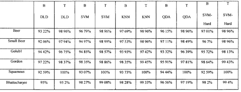
Table 2. Average of classifiers' perforances on bottom 10 (B) and top 10 (T) LS pairs.

Beer Small Beer Golubl Gordon Squamous Bhattacharjee B DLD 93 22% 92 06%

94 4 2 %

97 22%

92 59%

9 5 %

T DLD 98 96% 97 94% 96 75% 98 37% 100% 95 2% B SVM 96 79% 94 97% 94 85% 98 35% 93 07% 98 27% T SVM 98 96% 98 99% 98 57% 98 86% 100% 99 08% B KNN 97 69%

97 5 3 %

93 9 3 %

98 3 5 %

93 7 3 %

98 2 8 % T

KNN

98 96%

97 42%

99 4 5 %

100%

99 3 3 % B

QDA

96 15%

97 11%

93 32%

95 9 1 %

94 44%

96 56% T

QDA

98 96%

98 4 9 %

96 39%

97 8 1 %

100%

97 19% B

SVM-Hard

97 0 1 %

96 7%

95 72%

98 64%

92 5 9 %

98 2 % T SVM-Hard 98 96% 98 96% 98 13%

99 4 3 %

100%

99 4%

(41)

Table 3. Accuracy on the top three LS-pairs versus accuracy on the full gene set, using SVM with hard margin.

Small Beer

Beer

Squamous

Bhattacharjee

Gordon

Golubl

TP1

98 96%

100%

99 23%

99 83%

95 42%

TP2

98 96%

100%

99 56%

100%

TP3

98 96%

100%

99 74%

99.94%

100%

Full Data 100%

99.06%

100%

98 08%

99 28%

98 61%

Table 4. Accuracy on the bottom 3 LS pairs versus accuracy on the full gene set, using SVM with hard margin.

Small Beer

Beer

Squamous

Bhattacharjee

Gordon

Golubl

BP1

96 88%

96 46%

93 17%%

98.21%

98 78%

96 39%

BP2

96 98%

96 77%

92 93%

98 01%

98 56%

96 11%

BP3

96 15%

97 08%

92 68%

98 14%

98 45%

95 28%

Full Data

100%

99.06%

100%

98 08%

99.28%

(42)

<

A A O O O A O

< - * " <

A B

Figure 5. A set of points causing Linear Separability (Left Panel) Vs. Non Linear Separability (Right Panel)

^ o ) $S o 3 ^

A B

Figure 6. The projection of vectors of LS Points in the Zero-Sphere (Left Panel) Vs. Non Linear Separability (Right Panel)

1.2. LS-Genes Ranking Criterion

In mathematics, an n-sphere is a generalization of the surface of an ordinary sphere to an

arbitrary dimension. For a natural number, n, an n-sphere is defined as the set of points in

(n+l)-dimensional Euclidean space. As an illustration, a 0-sphere is a pair of points on a

line, a 1-sphere is a circle in the plane, and 2-sphere is an ordinary sphere in

three-dimensional space [30]. A single gene is an LS-gene if and only if all the m\ni2 vectors in

the corresponding 0-sphere point are in the same direction (See Fig. 5 and 6 for a non

LS-gene, a LS-gene and their projections in the 0-sphere). We use a simple ranking criterion

illustrated in Fig. 7: for each LS-gene, we compute the quantities A and B and use the

ratio AIB as the score of the LS-gene.

1.3. Search strategies for selecting LS genes and LS pairs

Gene subset selection approaches based on gene pairs have been proposed in [2]. For a

given gene pair, the authors used a two-sample ^-statistic on projected data samples as the

A

Rar*=A/B A A A A . _ Q O Q Q_

Figure 7. Ranking Criterion for LS Genes

(43)

score of pairs (pair /-score), and then pairs are ranked according to their /-scores for the

purpose of subset selection. They devised two subset selection algorithms, which differ in

the way gene pairs are selected for inclusion in a current subset. In their fastest method,

they iteratively select the top-ranked gene g, from the current list of genes, then find a

gene g, such that the /-score of the pair g,y = (g„ gj) is the maximum given all pairs g« =

(g„ gk), and then remove any other gene-pairs, containing either gt or g,; this continues

until r genes are selected. In their best, but very slow method, they generate and rank all

the possible gene pairs, and then select the top r ranked gene-pairs. The gene-pairs in [2]

are not necessarily LS-pairs.

In this section, we propose gene subset selection approaches based on selecting only

LS-genes and LS-pairs. The problem with this is that, initially, a data set may have a low

degree of linear separability, and hence, not enough LS-Pairs to select from. To overcome

this problem, we first apply SVM with soft margin on the initial given data set before

performing any gene selection method, and then sort the support vector (SV) samples in

decreasing order of their lagrange coefficients, obtained by training SVM; lagrange

coefficients are non-zero for support vector samples, which are farthest from the

separating maximum margin hyperplane and are probably misclassified. When there are

no more LS-features to select from during the process of gene selection, we then

iteratively remove the current SV sample having the largest Lagrange coefficient, until

the resulting data set contains LS-features; we devised three filtering methods to be

(44)

1.3.1. LS Approach

Our first gene subset selection method [11] proceeds by iteratively selecting disjoint

LS-pairs until a subset S of r genes is obtained. The LS-LS-pairs are ranked according to the

ranking criterion, which is already discussed. Given a gene expression data set D, our

first method is as follows:

LS; LS-Pair Selection on D;

1. S+-{}

2. r*— desired number of genes to select

3. d^-0

4. IfJ<rThen

a. P <— set of LS-pairs of D

b. P^P-igyS.t.g^SorgjcS}

c. Repeat

i. S <— S + {gy <— top-ranked LS-pair in P} ii. Apply a classifier on S and update Best-S iii. P *- P - {giJ s.t. g, e S or & e S}

iv. d *— d + 2

Unti\d>rorP= {}

5. IfJ<rThen

a. Repeat

i. D <— D- {SV sample with largest Lagrange coefficient} Until D contains LS-features

b. Repeat from 4 with the resulting D 6. Return S, Best-S, and their performances

In the LS algorithm, S is the subset to be found, r is the desired size of S, and P is the

sets of LS-pairs. In line 4.c.ii, we apply classifiers to the currently selected subset S to

keep track of the best subset Best-S of size < r. We use ten runs of ten-fold

cross-validation on S, and the algorithm returns subsets S and Best-S and their performances.

SV samples with largest Lagrange coefficients are iteratively removed from data set D, in

line 5.a.i, whenever there are not enough LS-pairs in the current D.

(45)

1.3.2. LSGP Approach

In the LS approach we only considered LS-pair, whereas our second gene subset

selection method proceeds by iteratively, selecting in this order, from the set of LS-genes

and then from the set of LS-pairs until a subset S of r genes is obtained. The LS-genes are

ranked according to the ranking criteria discussed above. Given a gene expression data

set D, our LSGP method is as follows:

LSGP: LS-Gene and LS-Pair Selection on D:

1. S « - { }

2. r <— desired number of genes to select

3. d+-0

4. G <— set of LS-genes of D

5. G<— G - {g, s.t. g, £ S}; ' - ' = set-difference 6. Repeat

a. S <— S + {g, *— top-ranked LS-gene in G} ; ' + ' = union

b. Apply a classifier on S and update Best-S c. G<-G-{g,}

d. d<-d+l

Until d=r or G={} 7. If d<r Then

a. P *— set of LS-pairs of D

b. P+-P-{g,Js.t.g,£SoTgleS}

c. Repeat

i. 5 <— 5 + {g,, <— top-ranked LS-pair in P} ii. Apply a classifier on 5 and update Best-S

iii. / > « - P - {gw s.t.g,eS or g,cS}

iv. d <— d + 2

Until <sf > r or P = { } 8. If<5?<rThen

a. Repeat

i. D <— Z> - {SV sample with largest Lagrange coefficient} Until D contains LS-features

b. Repeat from 4 with the resulting D

(46)

The difference between LS algorithm and LSGP algorithm is in lines 4 up to 7, in

which LSGP selects LS-genes. Moreover when a LS-gene g, (resp., LS-pair gab) is

selected, we also remove all LS-pairs containing g„ (resp., ga or gb); see lines 7.b and

7.c.iii. This deletion is in order to minimize the redundancy. That is, when LS-gene g, is

selected then any LS-pair containing g, will be redundant.

1.3.3. Graph-Based Methods

In [2] the authors first select the top-ranked gene g, and then find a gene g, such that the

pair g,j has maximal pair /-score. Also in their slow approach (which yields better

performance than their fast method) they iteratively select the top-ranked pairs in such a

way that the selected pairs are mutually disjoint from each other. That is, they delete all

of those pairs which intersect the currently selected subset of genes. Assume a LS-pair

gab = (ga, gb) is selected and assume LS-pair gbc - (gb, gc) £ P not yet selected. If we

remove gbc, then the possible LS-triplet g0*c = (ga, gb, gc), which may yield a better subset

S or a shorter subset Best-S, will be lost. Hence, we devised a third selection method for

selecting LS-features.

Let G be the set of genes, we generalize the definition of linear separation to apply to

any /-tuple gi , = (g,i, ga, • • •, gn) of genes where 1 < t < \G\, 1 <j < t, and i} e {1, ..., |G|},

and say that: g\ , is a linearly separating /-tuple (LS-tuple) if there exists a separating

(/-1 )-dimensional hyperplane H in the /-dimensional sub-space defined by the genes in g\ ,.

It remains open to generalize the theorem of [1] to /-tuples of genes, / > 1, by considering

projecting the m\Tti2 vectors obtained from the /-dimensional points onto a unit

(47)

sphere, and then determine a test for linearly separability of a Muple from the ( M )

-sphere. Clearly, the theorem is true for t=\: since a 0-sphere is a pair of points delimiting

a line segment of diameter 2, and that the m\m2 vectors point in the same direction (i.e.,

they form a sector of angle 0) if and only the single gene is linearly separable. Therefore

in our third method we consider the intersection graph N = (P, E) where, the vertex set is

the set of LS-pairs, P, in D and edges (v„ v,) £ E if v, and v, have a gene in common. We

then perform a graph traversal algorithm on N, which selects LS-pairs as the graph is

(48)

DF-LSGP: Graph-Based LSGP Selection on D

1. S ^ { }

2. r <— desired number of genes to select 3. rf<-0

4. G <— set of LS-genes of D

5. G*— G — {g, s.t. g, E 5}; ' - ' = set-difference ; remove already selected LS-genes 6. Repeat

a. S" <— 5 + {g, <— top-ranked LS-gene in G] ; '+ ' = union

b. Apply a classifier on 5 and update Best-S c. G*-G-{g,}

d. d<-d+\ Until rf = /• or G= {} 7. Ifrf<rThen

a. P <— set of LS-pairs of D

b. /,^ /,- { g , s . t .S£ G o r&e G }

; remove LS-pairs containing LS-genes c. />«-/>-{g„s.t.geSandgjeS}

; remove already selected LS-pairs d. Construct intersection graph N=(P,E) e. For each vertex gy: set visited [g,y] <— false

f. While there are un-visited vertices and d < r Do: i. Stack <-{}

ii. gy <— top-ranked vertex in TV

iii. Push g,j onto StocA:

iv. While Stack ± {} and d < r Do: 1. Pop g,y from Stack 2. If gy is un-visited Then

a. w's;ted[gy] <— true

b. rf^|S+{g„}| c. S^S+{glJ}

d. If S has changed Then

i. Apply a classifier on S and update Best-S e. P<- P - {g,6 s.t.g, eSandg*eS}

; cfe/e/e already selected vertices from N

f. Push all un-visited neighbors of gy onto Stack starting from the least-ranked ones.

8. Ifrf<rThen a. Repeat

i. D <— D- {SV sample with largest Lagrange coefficient} Until the resulting D contains LS-features

b. Repeat from 4 with the resulting D 9. Return S, Best-S, and their performances

(49)

2. r <— desired number of genes to select 3. d*-0

4. G <— set of LS-genes of£>

5. G<— G - {g, s.t. g, E 5}; ' - ' = set-difference

; remove already selected LS-genes

6. Repeat

e. S <— S+ {g, *— top-ranked LS-gene in G} ; '+ ' = union

f. Apply a classifier on S and update Best-S g. G - G - { » >

h. rf<-rf+1 Until rf = r or G={} 7. Ifrf<rThen

a. P <— set of LS-pairs of D b. i> < - P - {gy s.t. g, EGorg, t G j

; remove LS-pairs containing LS-genes c. / > « - / > - { g , s . t .ae . S and g,eS}

; remove already selected LS-pairs d. Construct intersection graph N = (P,E) e. For each vertex g,y. set visited [g,J <— false f. While there are un-visited vertices and d < r Do:

i. queue *— {}

ii. g,! <— top-ranked vertex in N iii. En-queue g,y onto ^«e«e

i v. While queue # {} and d<rT>o: 1. De-queue gv from queue 2. If gy is un-visited Then

a. rfHS+{g„}| b. S^S+t&j) c. If 5 has changed Then

i. Apply a classifier on 5 and update Best-S d. P <-P-{ga (, s.t. g.eS'and gj £S }

; cfetoe already selected vertices from N

e. En-queue all un-visited neighbors of g,y onto queue starting from the high-ranked

ones and change visited[gv] <— true

8. Ifrf<rThen c. Repeat

ii. D *— D- {SV sample with largest Lagrange coefficient} Until the resulting D contains LS-features

d. Repeat from 4 with the resulting D

(50)

The differences between our LSGP method and LSGP are in lines 7. In

DF-LSGP, the LS-genes are selected first as in the LSGP method. Then we iteratively select

the best LS-pair vertex and its un-selected neighbors in a depth-first manner; see line 7.f

and thereafter. This continues until the desired number of genes, r, is obtained. We have

also implemented a breadth-first traversal of the graph, BF-LSGP, where the neighbors of

a selected LS-pair are sent to a queue starting from the top-ranked ones. In practice, we

do not create an intersection graph N (line 7.d) given that P may be very large for some

data sets; we simply push or enqueue the top-ranked LS-pair from the initial P onto the

stack or queue (line 7.f.iii) then simulate the graph-traversal algorithm.

2. Recursive Feature Subset selection

Univariate filter methods, which rank single genes according to how well they each

separate the classes, are widely used for gene ranking in the field of microarray analysis

of gene expression datasets. These methods rank all of the genes by considering all of the

samples; however some of these samples may never be classified correctly by adding

new genes and these methods keep adding redundant genes covering only some parts of

the sample space and the returned subset of genes may never cover the sample space

perfectly. In this section we introduce a gene subset selection approach which aims to add

genes covering the sample space which has not been covered by already selected genes in

a recursive fashion.

(51)

_ A 4 A M A 4 _ _ o g Q Q 0 2 £ £ .

A. Samples of an LS Gene

Non-LS Samples

O O O O O O O C

A A A A A A A

B. Samples of a Non-LS Gene

Non-LS S a m p l e s

< < \ • *

_{0 2 0 0 , , , O Q O O Q Q p o}

Mm C 1

. - A

ttaxCI

C. Samples of a Non-LS Gene

N o n - L S S a m p l e s

poooooooo oo o o oo

t\Z\ ZI\Zi

Win C ? Max C 2

Min C 1 M W C 1

D. Samples of a Non-LS Gene

(52)

Our algorithm, first selects gene gt which can be selected by any gene ranking criteria

and then partition samples to those causing non-linear separablility and those causing

linear separablility based on the selected gene gt; then the algorithm recursively selects

gene gj causing good degree of separation based only on non-LS samples. The

motivation is that when some samples are linearly separable with gene #;, they will still

remain linearly separable by adding any other genes to gene gt. Hence our algorithm

focuses on those non-LS samples to find good degree of separation by adding gene gj.

Here first we introduce the definition of linear and non-linear separable samples and then

we propose our recursive algorithm.

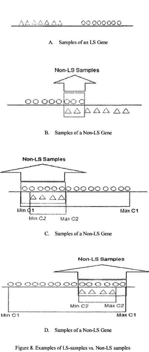
2.1. LS samples vs. non-LS samples

As said earlier we apply the ranking criterion on non-LS samples in a recursive fashion.

We partition the samples to LS samples and non-LS samples as shown in figure 8; the

intersection of classes is considered as non-LS samples (see fig 8.B for instance);

however when the intersection of two classes' samples is one of the classes (see fig 8.C

and 8.D for example), in this case, the non-LS samples are defined as follows:

If (Max (C2)- Min (CI)) < (Max (CI) - Mln(C2))

non-LS Points= Min (CI) <samples< Max (C2)

Else

non-LS Points= Min (C2) <samples< Max (CI)

End