Experimental Sensitivity Analysis of a Network Controlled Unmanned Ground Vehicle in iSpace

ABSTRACT

PELENTRIDES, IOANNIS. Experimental Sensitivity Analysis of a Network Controlled Unmanned Ground Vehicle in iSpace. (Under the direction of Mo-Yuen Chow.)

Experimental Sensitivity Analysis of a Network Controlled Unmanned Ground Vehicle in iSpace

by

Ioannis Pelentrides

A thesis submitted to the Graduate Faculty of North Carolina State University

in partial fulfillment of the requirements for the Degree of

Master of Science

Electrical Engineering

Raleigh, North Carolina 2007

APPROVED BY:

_______________________ _______________________ Dr. Liu Xun Dr. James J. Brickley

DEDICATION

To my parents Christos and Myroulla

for their continuous love and support

BIOGRAPHY

Ioannis Pelentrides was born in Limassol, Cyprus on November 9th, 1978. He finished his secondary education studies in 1996 and he was admitted in the Electrical and Computer Engineering Department of the National Technical University of Athens, Greece in 1998.

He joined the Cyprus National Guard in July 1996, where he was selected to serve as a cadet and he was promoted to second Lieutenant in May 1998.

ACKNOWLEDGMENTS

I would like to express my deepest appreciation to my advisor, Dr. Mo-Yuen Chow, for his invaluable guidance and support throughout this work. His deep knowledge and expertise on this subject were priceless assets for my research. I would also like to thank my committee members, Dr. James J. Brickley and Dr. Xun Liu, for their willingness to discuss my work and their useful feedback. My sincere appreciation also goes to all members of the ADAC Lab; the discussions we had helped me overcome issues that emerged during my work and implement my ideas in a useful manner.

I am very grateful to Dr. Yannis Viniotis for the financial support he provided me during the last months of my studies.

The basic knowledge of Control Theory and the experience I gained during my studies at the National Technical University of Athens, Greece are solely attributed to Prof. Paraskevas Paraskevopoulos. I consider myself privileged to have attended his lectures and learned from him.

TABLE OF CONTENTS

LIST OF FIGURES ... vii

LIST OF TABLES ... viii

SECTION I: INTRODUCTION...1

SECTION II: SENSITIVITY ANALYSIS AND NETWORKED CONTROL SYSTEMS...6

2.1 SENSITIVITY ANALYSIS... 6

2.1.1 APPLICATIONS – IMPORTANCE... 8

2.2 NETWORKED CONTROL SYSTEMS... 10

2.2.1 HISTORY... 10

2.2.2 APPLICATIONS – ADVANTAGES... 11

2.2.3 CURRENT RESEARCH... 12

SECTION III: SA OF A UGV IN ISPACE...14

3.1 SYSTEM DESCRIPTION... 14

3.2 PROBLEM DESCRIPTION... 18

3.3 PROBLEM FORMULATION... 20

SECTION IV: DESIGN OF EXPERIMENTS...22

4.1 MEASURABLE OUTPUTS... 23

4.2 INPUT FACTORS... 26

4.3 RANGE OF TREATMENT VARIATION... 32

4.4 FACTORIAL DESIGNS... 33

4.5 PILOT EXPERIMENT... 36

SECTION V: DATA ANALYSIS AND DISCUSSION...38

5.1 EXPERIMENTAL SETUP... 38

5.2 REGRESSION ANALYSIS... 40

5.2.1 REGRESSION MODELS FOR THE DEVIATION ERROR... 43

5.2.2 REGRESSION MODELS FOR THE COMPLETION TIME... 45

5.3 RESULTS AND DISCUSSION... 48

5.3.1 MODELS FOR THE DEVIATION ERROR... 48

5.3.2 MODELS FOR THE COMPLETION TIME... 51

5.3.3 MODELS FOR THE ROOT ERROR-TIME PRODUCT... 52

SECTION VI: CONCLUSION...55

REFERENCES ...57

APPENDICES ...62

APPENDIX A: ANA2 SPEED CHARACTERISTICS...63

APPENDIX B: FRACTIONAL FACTORIALS...67

LIST OF FIGURES

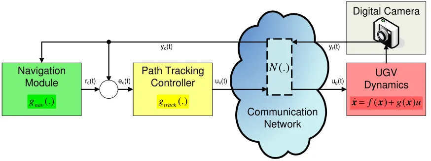
FIGURE 1 NETWORK CONTROLLED UGV SYSTEM...15

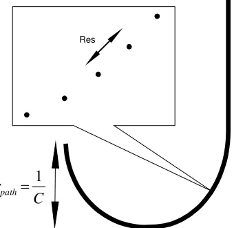
FIGURE 2 PRE-DEFINED PATHS’ SHAPE...16

FIGURE 3 DEFINITION OF TRACKING ERROR...19

FIGURE 4 DISTANCES OF THE VEHICLE FROM THE PATH...24

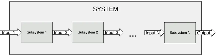
FIGURE 5 ABSTRACT REPRESENTATION OF A SYSTEM...27

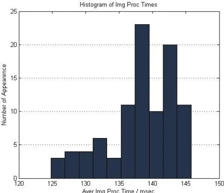
FIGURE 6 HISTOGRAM OF IMAGE PROCESSING TIMES...31

FIGURE 7 ISPACE IN ADAC LAB AT NCSU...39

FIGURE 8 DIFFERENT POSITIONS OF THE UGV ON THE PATHS...39

FIGURE 9 ANA2, ONE OF THE UGVS IN ISPACE...63

LIST OF TABLES

TABLE 1 IDENTIFIED SOURCES OF VARIATION...27

TABLE 2 FACTORS AND RESPECTIVE TREATMENT LEVELS...34

TABLE 3 FULL 34 FACTORIAL DESIGN...36

TABLE 4 PILOT EXPERIMENT’S RESULTS...37

TABLE 5 EXPERIMENTAL RUNS AND MEASUREMENTS...42

TABLE 6 MODELS FOR THE DEVIATION ERROR...49

TABLE 7 MODEL FOR THE COMPLETION TIME...51

TABLE 8 MODEL FOR THE COMPLETION TIME...53

TABLE 9 TIME, DISTANCE MEASUREMENTS FOR 6 SPEED LEVELS...65

TABLE 10 AVERAGE SPEED AND MAXIMUM DEVIATION ERROR...65

SECTION I: I

NTRODUCTION

Globalization once thought of as the expansion of human population and the growth of civilization[48] was “re-defined” by Theodore Levitt, a professor at Harvard Business School, in 1983[25]. The term now is used to express the establishment of communications, information exchange and human relationships on a global level and in many different forms. In virtually all areas of human activity, from business and industry to academia, politics and even religion, one can find several situations where this term can describe the way people trade, share, interact and communicate. The most influential scientific areas, whose advances led to the current globalization state, are networks and

communications. These, combined with the remarkable advances in computer systems, software, database design and management and the Internet, support Thomas Friedman’s words: “Globalization 3.0 (which started around 2000) is shrinking the world from a size small to a size tiny and flattening the playing field at the same time”[15].

Networked Control Systems (NCS) are currently deployed in many industrial facilities to enhance their functionality[45]. Industrial automation and intelligence is accomplished based on the introduction of networked control loops in the factory production lines[50]. Military and aerospace research focuses on NCS, as these systems provide many advantages to benefit from[51]. Tele-operations are now extended into the biological and the biomedical fields[46], while applications of NCS in many aspects of human activity are constantly studied and developed.

whose defining characteristic is the existence of a communications network in the control loop, parameters like network delay, data drop-rate congestion, bandwidth limitations and security protocols applied are of special interest. The performance of such systems, that is how well they serve the application that uses them, depends on the parameters mentioned and also on its operating conditions, environment, etc.

globe, the SA issue discussed in this thesis has not yet been explored to the level that it deserves.

Viewing the system from a sensitivity perspective can provide insight into the effect exerted by the network on the system under different operating conditions. We utilize the DOE (Design Of Experiments) methodology to design an appropriate experiment and, through regression analysis, to analyze the sensitivity of the system with respect to some of its parameters. Considering parameters from the network and different operating conditions, we draw quantitative and comparative conclusions about the NCS’s sensitivity.

We first define three performance measures (cost functions), which are used to characterize the system. They are the deviation (or tracking) error, which indicates the accuracy of the vehicle path tracking, the completion time (or system’s runtime), which measures the time needed for the vehicle to reach its destination and complete its task and the error-time product, which reflects the existing trade-off between path-tracking accuracy and system’s quickness.

Regarding the tracking error, it is shown that a linear model cannot sufficiently represent the system’s behavior. A more complex model, which includes second-order interactions between the four parameters studied, is developed instead. Independent data processing indicates a quadratic relation between the deviation error and the maximum look-ahead distance. We include the corresponding quadratic term in our model and, through regression analysis, we show that such a relation can well explain part of the system’s observed behavior. It is shown that due to the higher order effects involved in the model, the sensitivity of the system to its parameters can be described by a set of linear equations. These equations can provide local information about the relative importance of the parameters studied on the deviation error at a given operating condition.

The completion time cost function measures how fast the vehicle completes a given task. The derived model supports our initial assumptions on the impact of the vehicle’s speed, the look-ahead distance and the network’s delay. The sensitivity values derived for these parameters are much larger than the one derived for the curvature, and thus, we can conclude that the latter does not have any major effect on the completion time.

almost equal, but opposite, effect that the network delay and the look-ahead distance have on the product value. We elaborate on this observation in the last section of our work.

SECTION II: S

ENSITIVITY

A

NALYSIS AND

N

ETWORKED

C

ONTROL

S

YSTEMS

2.1

Sensitivity Analysis

It is a common practice for engineers to model the systems they design and then simulate their operation before the actual implementation of their designs. Scientists working in many different scientific disciplines undertake similar actions in order to prove new theorems or to establish their ideas. Models are usually used when running experiments on actual systems is expensive, when the systems are not easily reachable, or when the system is in the design process and not completed yet.

The importance of models, which are developed to mimic the behavior of a system, can be further emphasized if we consider all the economic, sociological and biological models, which are developed in order to explain the current situation of the respective systems but most importantly predict how these systems will evolve in the future, what issues may arise during their evolution, and which are the most effective ways to resolve them. Strongly related to modeling, SA provides the tools through which understanding and explaining real systems is achieved. “Sensitivity Analysis is the study of how the variation in the output of a model (numerical or otherwise) can be apportioned, qualitatively or quantitatively, to different sources of variation and how the given model depends upon the information fed into it”[32].

a. If the model resembles the system under study. SA results may suggest that the model exhibits strong dependencies on factors that were supposed to be non-significant. In this case, the model should be considered inappropriate to reflect the system’s operation and it should be revised.

b. Which factors cause most of the output’s variability? Identifying the factors that have the most “dominant” effects on the output of the model, can lead to minimizing measurement errors on computational results by optimizing the most influential factors in the model.

c. Which are the insignificant parameters in the model. Non-significant factors, in the sense of not causing important variation in the output, can be neglected from the model so that its complexity is reduced and its study becomes easier.

d. If there exist optimal regions within the input ranges. Defining optimal regions for the factors can provide the means for calibrating the system and also predict to which extend the model’s results effectively reflect the real system’s behavior.

2.1.1 Applications – Importance

Viewing sensitivity analysis as a generalized tool, which is utilized to provide important information about a system, one can speculate that it can be applied in many different fields. This is actually a rather conservative assumption. Applications of sensitivity analysis can be found in almost every aspect of human activity, and if there exist areas in which SA is not applied, it shouldn’t be due to the lack of appropriate methods but most probably because necessity for SA did not occur. The wide range of areas, which benefit from sensitivity analysis, can be demonstrated by the abundance of relevant papers in the literature. Sensitivity analysis studies have been performed in order to optimize an ultrasonic linear motor[14], separate chemical compounds in hypertension drug studies[2], develop robust, insensitive to manufacturing tolerances induction motors[5], retrieve soil moisture from a microwave emission model[8] and make decisions in a multi-objective evolutionary optimization problem[3]. SA in other scientific areas, such as economics[9], education[16] and political science[18] may also be found.

in addition, the inputs and the available data are affected by uncertainty, quantitative SA can be performed to provide confidence levels for each parameter included in the model. These result in reducing the efforts made in system tuning procedures.

When used to validate an already existing model, SA can provide information on the effectiveness of the model in replicating the system’s behavior. Modeling a system requires consideration of certain parameters as non-significant and exclusion of them from the final model. The results of a SA study might suggest, however, that the hypotheses made for these parameters are not correct. This would lead to deriving a more realistic model. On the other hand, if a model is more complex than it should be, SA can pinpoint the non-significant factors, which can be excluded from the model through “mechanism reduction”.

2.2

Networked Control Systems

Our work has been conducted in a networked environment. This implies that any analysis related to the performance of the system should include parameters imposed by the communications network. There exist many similar definitions of the NCS. A descriptive definition, found in[47] states that: “When a traditional feedback control system is closed via a communication channel, which maybe (sic) shared with other nodes outside the control system, then the control system is called a Networked Control System (NCS)”.

Considering the system we have studied, we should note that the path-tracking problem has been studied for years, and several control methodologies have been successfully developed and implemented to improve the performance of such systems. Based on adaptive[12] or robust[1] theory, on fuzzy[20][26] or predictive[22][36] algorithms and other control methodologies, several designs assuring good levels of tracking performance have been developed. However, under a networked control environment, methodologies designed for traditional systems usually fail to achieve the desired performance levels. The existence of the communications channel in the feedback loop introduces several constraints on the system’s functionality, which are discussed in later paragraphs.

2.2.1 History

first attempt to interconnect systems using a dedicated communications network. A CAN protocol was then implemented in hardware, using Intel’s 82525 chip, which found use in many different applications. The CAN, although successfully implemented, did not cause any major changes in communications because of its local usage. Deployment of wireless networks and the Internet, however, changed dramatically the way communications were made or even understood. Accessing and sharing information from remote locations very soon created new, exciting and challenging research fields, and many opportunities for advanced applications. The advantages of wireless communications over the traditional networks were obvious from the beginning, while accessing the Internet through the wireless infrastructure was a promising feature.

2.2.2 Applications – Advantages

the two technologies with control theory can result in very exciting, high-tech applications[34].

Industrial automation has undoubtedly absorbed much of the NCS development impact[4]. Production lines in manufacturing plants are transformed into NCS, and they are monitored and controlled by designated personnel through the Internet. In the medical field, simulations of robotic equipment performing tele-surgeries are currently being studied[6], so that real-time operations will be feasible in the future. With the development of the human-machine interface (HMI), specially designed robots can perform several tasks in response to minimal movements of an impaired person’s body [37]. Military operations can benefit from the use of unmanned ground or aerial vehicles in specific missions[21][39]. The list of potential applications of NCS is very long.

2.2.3 Current research

In[27], the emergence of industrial networks for control, diagnostics and safety are explored and the impacts of the devices’ performance in assessing the network performance are developed. Networks’ data-rate constraints on feedback control are examined in[28]. Similar research is conducted in[19] along with other open research fields like state estimation over imperfect communications channels, the closed-loop stability of NCS in the presence of sampling, delays and packet dropouts and the effect of system’s architecture on the performance of NCS. A deeper study for network architectures can be found in[7].

SECTION III:

SA

OF A

UGV

IN I

S

PACE

This thesis focuses on the Sensitivity Analysis study for the UGV path-tracking problem in a network based control environment. The study conducted in ADAC iSpace, a platform that provides necessary modules for the analysis, aims to identify the parameters that affect the performance of such a system in terms of tracking error and time taken for completion of a task. This study can provide information about the dependencies existing within similar systems and therefore, the conclusions can be representative for applications involving similar forms of navigation systems. Being aware of the parameters that have the most significant effect can help in the design process of such systems. More emphasis can be given in controlling parameters, which have major effect in performance degradation, while less influential parameters can be given less consideration, at least during the first phases of the design process.

3.1

System description

perform a SA study, all these system components must be analyzed so that all possible influential parameters can be extracted from them.

Digital Camera

yr(t)

Navigation Module (.) nav g Path Tracking Controller (.) track g UGV Dynamics ec(t)

rc(t)

(.)

N

uc(t) ug(t)

yc(t)

Communication Network

( ) ( )

x=_f x +_g x _u

Figure 1 Network Controlled UGV System

This study involves a specific type of unmanned ground vehicles, namely the differential drive UGVs. The dynamics of such vehicles are governed by[42]:

Τ

1 2 1 2

( )

( )

[

]

x

x

x

x

f

g

u

x y

θ θ ω ω

=

+

=

(3.1)

where (x,y) are the coordinates of the vehicle, θ_1,θ_{2 are the displacements of the left and}

right driving motors respectively and ω_1,ω_{2 are the rotational speeds of the left and right}

wheels. Control of the vehicle is achieved by sending appropriate control signals to the vehicle. These signals consist of two integer values, the first corresponding to the desired forward speed of the vehicle and the second corresponding to its desired rotational speed. These values are translated into pulse-width modulated voltage signals by the vehicle’s microcontroller, which are used as the motors’ input signals.

parameters. If security is included in the data transmission protocol, then it should also be included in the list of network parameters.

The navigation module is used to determine the reference point on the path towards which the vehicle should be driven. In order to determine this, it considers the current position of the vehicle (x0,y0), the path’s curvature (C) and the maximum

look-ahead distance (dmax). The path defined in this study is a straight line followed by a

semi-circular curve. In our implementation these two segments were not defined as two continuous lines. Instead, we defined the path as a sequence of points, where consecutive points where a constant distance apart from each other (Figure 2). Considering this information the path is described by:

( ,

, )

Path

p s Res C

where s is the length of the straight-line segment, Res is the distance between two adjacent points (resolution) and C, is the curvature of the semi-circular segment.

Res

1

path r

C =

Figure 2 Pre-defined paths’ shape

The maximum look-ahead distance, dmax, is a user-defined parameter, which

commanded to travel during the next iteration of the control algorithm. Referring to eq. 3.3, ds is the distance on the path that the vehicle is planned to travel. C is the path’s curvature and α_{1 is a positive constant. For a given value of} α_{1, the planned distance will} be equal to the maximum look-ahead distance only if the path’s curvature is zero. As the curvature of the path increases, the look-ahead distance will decrease. The next reference point is then determined considering both the calculated look-ahead distance and the current position of the vehicle.

max

1

1

*

d

ds

a

C

=

+

Considering the above we describe the function of the navigation module as:

(

)

(

,

,

,

,

)

(

,

)

nav ref ref ref

g

x y

d

α

C

→

r

=

x

y

The path-tracking module is responsible to generate appropriate control signals, which will drive the vehicle towards the reference point. The quadratic path-tracking algorithm used in ADAC iSpace can be represented by:

(

)

(

,

,

,

)

,

track x y ref ref

g

ε ε

V

α

→

V

Tr

where (ε_x,ε_{y) is the error between the current and the reference position in the x- and}

y-dimensions, Vmax, is a controlled variable representing the maximum allowable speed of

the vehicle and α_{2is a control variable used to adjust the vehicle’s speed according to the}

path’s curvature, Vref and Trref are the calculated reference speed and turn rate that would

3.2

Problem description

As mentioned in the introductory Section of this study, sensitivity analysis is a statistical tool, utilized to extract information about the dependencies that exist between the inputs and the outputs of a system. In the UGV path-tracking problem, an autonomous vehicle is controlled over a network in order to follow a predefined path. Ideally, the vehicle would move right on the path. In practice, however, due to measurement errors, physical constraints and other uncontrolled parameters, some deviation error occurs. Several control variables are included in the control algorithm designed to guide the vehicle along the desirable path. These variables can affect the performance of the system, as they are involved in the calculation of the control signals sent to the vehicle. While parameters involved in the algorithm can be easily controlled, other factors also inherent in the system, however random in nature, constitute a set of uncontrollable variables that also affect the system’s performance. The communications network used in iSpace, Ethernet and Wireless UDP, is the source of these random parameters. Time-delay, data dropout and limitations on the available bandwidth can be responsible for the system’s degradation or even, under certain circumstances, destabilization.

should be straightforward; by definition, the path-tracking problem involves controlling a vehicle to follow a desirable path. The deviation error can provide information about how well the vehicle tracks the path. It can be defined as:

( )

( )

dev s

E

=

∫

p x

−

t x dx

where s represents the range of the vehicle’s movement along the x-axis and p(x) and t(x)

are functions describing the equations of the designed path and the actual path tracked by the vehicle respectively.

-0.2 -0.1 0.1 0.2 0.3

-0.2 -0.1 0.1

x

y

Tracked Path: t(x)

De signed Path: p(x)

Figure 3 Definition of Tracking Error

Driven by the time-sensitive applications of NCS, we define a second performance measure, which considers the total time taken for the vehicle to reach the end of the path. This is defined by eq. 3.7:

tot end start

T

=

t

−

t

between tracking accuracy and system’s quickness. This measure (eq. 3.8) can be generally used for comparing different systems, which have similar functionality but are implemented following different approaches.

*

ET dev tot

Prod

=

E

T

3.3

Problem formulation

This section provides a formulation of the SA problem in a mathematical framework, to establish the basis for the rest of our study.

Let A = [a1, a2, … , ak]T be the kx1 vector of the input parameters that are believed

to have some effect on the system’s performance. For example, if it is believed that the vehicle’s speed and mass and the network delay and bandwidth are the only four parameters that effect the system’s performance, the vector A would be defined as:

A

V

M

T

BW













=













Let us now define Si = Hi(A), i=1, 2, …, n to be the ith-performance characteristic

for the system. This characteristic is described by the function Hi(.) of the input

parameters’ vector, A. In general, this function can belong to any set of the real-valued functions; however, to avoid any mathematical implications, we consider Hi(A) to be a

2

1

(

,

,

,

)

H V

M

T

BW

=

x

+

x V

+

x V

+

x M

+

x T BW

where xi’s are the real-valued coefficients of the parameters.

In this experimental sensitivity study the functions Hi(A) are not known. Let us

consider the function,

ˆ

_{ˆ ( )}

A

_1,2,...,

i i

S

=

H

i

=

n

to be an estimated expression for the ith-performance characteristic. Taking partial derivatives of this expression with respect to the input parameters we get:

( )

1 2

ˆ

ˆ

ˆ

ˆ

ˆ

ˆ

_,

_,

_,

_,

_1,2,...,

T

i i i i

k

S

S

S

S

V S

i

n

A

a

a

a





∂

∂

∂

∂

=

=

_

…

_

=

∂

_

∂

∂

∂

_

We consider

ˆ

S

a

∂

∂

with respect to its ith-performance characteristic based on the following reasoning:

When the estimations,

S

ˆ

partial derivatives, with respect to inputs aj, are constant values, which represent the rate

of change of

S

ˆ

outputs by unitary changes in its inputs, which in turn, is the definition of a system’s sensitivity.

In case the estimated functions of Si’s are not linear, their partial derivatives will

SECTION IV:

D

ESIGN OF

E

XPERIMENTS

We utilize DOE methodology to design and implement an experimental procedure, whose results will be used to derive the desired estimations of the system’s performance measures (eq. 3.10). Design of experiments is a methodology developed for researchers, professionals and other individuals, who are involved in developing systems’ models or in identifying systems’ characteristics. These procedures usually involve running simulations or experiments, gathering appropriate data and then analyzing them to draw conclusions. It is important for the experimenter, to spend sufficient time, prior to experimentation, to organize his/her activities so that a simple and condensed experiment is designed. It is the goal of experimental design to minimize the allocated resources spent during the experiments, these being time consumed, personnel involved or raw material used. From an academic point of view, research and experiments might not be very time-critical. However, when it comes to applications in industry where time is a very important recourse, design of experiments can be used as a tool for extracting the desired information while minimizing the overall cost of doing so. In the following paragraphs, all considerations made during this experimental design will be analyzed and the final experiment will be described.

to be extracted. For this, we first identify all possible sources of variation. Treatment factors, which are the set of parameters of interest, are extracted out of the population of the sources of variation and then, respective ranges of variation are defined for each treatment. The experimental units, which would be subjected to the treatments’ levels and noise factors, which are random variables inherent or external to the system, are also defined prior to experimentation. The experimental procedure, the measurements to be made and some anticipated results are considered as well. In general, DOE suggests running pilot experiments if the system’s behavior or characteristics are not precisely known to the experimenter. Such experiments can provide information about the effectiveness of the procedure used, a suitable model for the system and also elicit any latent issues. Finally, based on the assumed model, appropriate data analysis should be performed. For the SA study we are concerned, regression analysis is utilized to provide the desired information for the sensitivity functions. We start the experimental design by defining the output measurements we intend to collect. Then we discuss the input factors considered, their ranges of variation and we also describe the pilot experiment along with its outcomes in the following paragraphs.

4.1

Measurable Outputs

cannot be achieved. Therefore, at every instant, the vehicle would be some distance away from the desired path. To find the shortest distance of the vehicle from the path, we consider the perpendicular to the path, which passes through the vehicle’s center. The point at which this line intercepts the actual path defines the shortest distance of the vehicle from the path. In Figure 4, the vehicle is shown at two different positions with respect to the path. D1 and d2 are the shortest distances of the vehicle from the path when it tracks the straight and the semicircular segments respectively.

d1

d2

Figure 4 Distances of the vehicle from the path

1 1 1 1

(

)*(

)

2

k k k k

k

path

d

d

s

s

S

L

− −

=

+

−

=

∑

where S1 is the normalized total error, dk is the shortest distance at the kth-iteration, sk is

the path point closest to the vehicle at the kth-iteration, Lpath is the total length of the path

measured in meters and kt measures the times the control algorithm is repeated.

The total time taken for the vehicle to reach its destination is the second output of interest (eq. 3.7). We expected this performance measure, however, to be tightly dependent on the delay of the network, which is random in nature. In order to design a controllable experiment, our algorithm should be able to compensate for the network’s randomness. To design a more robust algorithm we first considered that the network’s effect is mostly reflected in the image processing time. This is the time taken for the sensors to capture, process and send the images to the controller. In our algorithm we:

measure the image-processing time for every iteration of the algorithm measure the total time taken for the vehicle to reach its destination subtract the total image-processing time from the system’s total run time Having these in mind the completion time is calculated as:

2

end start img

path

t

t

S

L

τ

−

−

=

∑

where, S2is the system’s run time and Στimg is the total image processing time. Dividing

We then define a third performance measure, the error-time product. This is a function that represents the existing trade-off between tracking accuracy and system’s run time. To decrease the run time we need to drive the vehicles at higher speeds. However, we can intuitively assume that this would result in increased deviation error. On the other hand, to increase the accuracy we might need to use more complex image processing algorithms. The additional computational burden imposed by them might require the vehicles to be driven at lower speeds. This in turn would increase the system’s run time.

The above reasoning supports our selection of the error-time product as a third performance measure. As this is a heuristic measure, no direct measurement of some system’s output could be utilized to provide information about its value. However, according to eq. 3.8 we can calculate its values by multiplying the tracking error and the system’s runtime at every experimental run. We describe this measure as:

3 1

*

S

=

S

S

4.2

Input factors

SYSTEM

Subsystem 2

...

Subsystem 1 Input 2

Input 1 Input 3

Figure 5 Abstract representation of a system

In this case, the output of one entity (sub-system) serves as the input to the following one. When conducting sensitivity analysis, it is these input (treatment) factors’ effects that we are interested to study. Depending on the complexity of the system, the process of identifying input factors can be fairly easy or maybe very challenging. For the particular problem several input factors are identified (Table 1). Because of the relatively large number of factors some of them were considered as “non-interesting”, so that the experimental runs needed are kept to a minimum. The selection is based on criteria like the nature of the input factors, the dependencies among them and some assumptions made to simplify the system’s model.

Table 1 Identified sources of variation

# Candidate sources of variation # Candidate sources of variation 1 Time delay (τ_{net) 6 Vehicle’s speed (Vmax)}

2 Available bandwidth (BD) 7 Look-ahead distance (Dmax)

3 Data dropout rate (δ_{d) 8} α_{1 (path-tracking variable)} 4 Path resolution (Res) 9 α_{2 (path-tracking variable)} 5 Path curvature (C) 10 Image processing time (τ_img)

The first three sources of variation are related to network QoS. The assumptions made for these parameters are:

Network time delay is constant

Data dropout rate is constant

Under these assumptions, a simple model for the network can be derived. In specific, a time-delay parameter, representing both the effect of the actual delay and the data dropout rate, can be assumed. Availability of bandwidth, although not guaranteed, is assumed to be sufficient and to support this assumption all experiments were scheduled during evening hours, when the local network in ADAC lab had less traffic. Therefore, the first input factor defined for the experimental design is the network’s combined delay, τ_del.

The resolution of the path was chosen to be equal to the resolution of the camera sensors, which capture images of the working area. Since one image’s pixel corresponds to 7.5mm, increasing the resolution on the path would not provide any additional accuracy on the measurements. The assumption that the path’s resolution does not have a major effect on the performance was then made and this source of variation was not included in the treatment factors.

On the other hand, path’s curvature is assumed to be a major source of variation. It is expected that paths with higher curvatures will have increased deviation error. The effect of the curvature on the completion time was not expected to be significant. This is the second treatment factor considered for the SA.

The third input factor considered in the analysis was the maximum speed of the vehicle, Vmax. Similar to the path’s curvature, it was expected to observe more deviation

obvious reasons. Considering the third performance measure, the product of the deviation error with the completion time, we anticipated some nonlinear relation for the speed. As this measure represents the tradeoff between tracking accuracy and time to completion, we can assume an optimal speed value, Vopt, to exist. Speeds lower than Vopt would

sufficiently increase the completion time, while higher ones would increase the deviation error in a way such that their product would always be higher than the one observed for the nominal value.

The maximum look-ahead distance, Dmax, is a parameter inherent in the quadratic

curve, path-tracking method used for guiding the vehicle. It defines the maximum distance on the path towards which the vehicle should be driven. The algorithm considers this distance and then provides the coordinates of the next reference point to be tracked. The expected effect is increased tracking error as Dmax increases. The look-ahead distance

can be seen as a straight line used to approximate a circular arc. The longest the line the worse the approximation would be, thus explaining our assumption for this factor’s effect. On the other hand, the further away the vehicle is sent, the faster it would reach its destination. This will result in shorter completion times. Therefore, similar to Vmax

regarding the third performance measure, a non-linear effect for the look-ahead distance can be anticipated.

non-significant for the analysis because in a real implementation, their values would be calculated once, perhaps based on some optimization method, and then remain unchanged. Additionally, we could assume that maximum speed and look-ahead effect could be combined with these parameters’ effect thus, making unnecessary any additional computational efforts.

to random disturbances occurred in the network, which were assumed insignificant enough to be ignored from the analysis.

Figure 6 Histogram of Image Processing Times

Based on the above results and to compensate for its effect, we considered the image processing time to be constant at 150ms throughout the experiments. When applying the desired value for the combined time delay, τ_{del, the following logic was} implemented:

(

150

)

del img

while

T

do

increase T

τ

τ

<

+

−

4.3

Range of treatment variation

The four treatment factors of interest, defined in the previous section, are: a combined time-delay, τ_{del, the vehicle’s maximum speed, Vmax, the maximum look-ahead} distance, Dmax and the path’s curvature, C. For these four parameters specific ranges of

variation were specified in order to design a fixed-effects factorial experiment.

The range defined for the time delay was based on data acquired in previous experiments[38] involving the control of a UGV in Japan from USA. Because of the long distance between the two locations, we assumed that the measured time-delays could be representative of many applications, which use similar technology and are run under similarly controlled conditions. A maximum value of 186ms was sufficient to model the network delay in IP communications while 124ms and 62ms were used to assure equally spaced levels within the treatment.

The maximum speed of the vehicle was assigned three levels as well. The selection process started with a small experiment designed to provide information about the speed range of the vehicle used in the experiments (Appendix A). As the results from this experiment suggested, a linear region of operation exists between 5cm/s and 15cm/s (Figure 10). Using these values as the two extremes, the third level for Vmax selected was

10cm/s. This value also provided equally spaced treatment levels for Vmax.

were highly distorted towards the edges we considered using only the central 1.5x1.0m part of the area. Then considering the paths’ shape we defined the smallest curvature to be 1.33m-1 (radius of 75cm) so that the longest distance between any points on that path would be 1.5x1.05m. The biggest curvature was defined to be 4m-1 (radius 25cm). We concluded on this value considering the size of the vehicle used for the experiments. The axis connecting the driving wheels of the vehicle is 19cm long and the rear wheel is located at about 18cm away from the axis. Therefore, setting the radius at 25cm was expected to provide some good information about the system’s performance at high curvatures and it also allowed us to define the mid-level for this treatment at 2m-1 (radius of 50cm).

Finally, the decision on the levels of the maximum look-ahead distance was taken considering the lengths of the paths. The longest path would be about 2.66m and the shortest one about 1.09m long. We have set the three treatment’s levels at 10, 20 and 30cm. The maximum value corresponds to about ⅓ _{of the shortest path, whereas the} minimum value is about 27 times smaller than the length of the longest path. Although these values are not calculated based on some constraints, we assume that they suffice to capture the effect of the look-ahead distance both on the tracking accuracy and the completion time.

4.4

Factorial designs

V (max. robot speed), D (max. look-ahead distance) and C (path curvature), they are all studied at 3 levels; the two extreme values defining the range of operation and their midpoint (Table 2).

Table 2 Factors and respective treatment levels Factor Time-delay

(T)

Max. speed (S)

Max. look-ahead (D)

Curvature (C)

Level1 62ms 9cm/s 10cm 1.33m-1

Level2 124ms 12cm/s 20cm 2m-1

Level3 186ms 15cm/s 30cm 4m-1

In a factorial experiment, all different combinations of treatments must be considered and experimental runs for each treatment should be conducted. The number of experiments needed is calculated as the number of the levels for each factor powered to the number of factors. Doing this results in 34 = 81 different combinations. As this number is relatively large and much time might be needed to conduct all the experiments, a fractional factorial design was investigated (Appendix B) in order to decrease the number of experiments to 27.

However, due to the relatively small amount of treatment factors, such a design would result in confounding of main effects with 3rd order ones and of 2nd order effects between them. This means that we wouldn’t be able to isolate the main effects from some important 3rd order interactions, or we wouldn’t be able to determine which 2nd order interactions are important. As a result, there was no other choice but to proceed with the full factorial experiment.

the 81 treatment combinations. Two measurements for each combination were scheduled, summing to a total of 162 experimental runs. The time taken for the experiments could be estimated considering the defined parameters’ values. The longest run would occur at maximum speed of 9cm/s and path curvature of 1.333m-1. The pilot experiment showed that an overall average of 8.6s per run could be anticipated. The time taken to record the results and reconfigure the vehicle was estimated to be about 60sec. Therefore, an estimate of the total duration of the experiments was calculated to be about 3hours. Using a 1/3 fractional factorial design might require only 1hour of experimenting, however, the

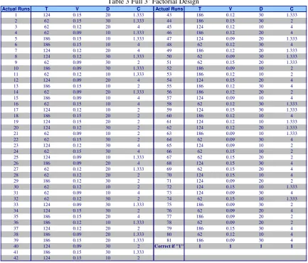
Table 3 Full 34 Factorial Design

Actual Runs T V D C Actual Runs T V D C

1 124 0.15 20 1.333 43 186 0.12 30 1.333

2 62 0.15 30 1.333 44 186 0.15 30 2

3 62 0.12 20 4 45 124 0.12 10 4

4 62 0.09 10 1.333 46 186 0.12 20 4

5 186 0.15 10 1.333 47 124 0.09 20 1.333

6 186 0.15 10 4 48 62 0.12 30 4

7 124 0.12 20 4 49 186 0.12 20 1.333

8 124 0.12 30 1.333 50 62 0.09 30 1.333

9 62 0.09 30 2 51 62 0.15 20 1.333

10 186 0.09 30 1.333 52 186 0.09 10 2

11 62 0.12 10 1.333 53 186 0.12 10 2

12 124 0.09 20 4 54 124 0.15 20 4

13 186 0.15 10 2 55 186 0.12 30 4

14 62 0.09 20 1.333 56 186 0.12 20 2

15 186 0.09 10 4 57 124 0.09 10 4

16 62 0.15 10 4 58 62 0.12 30 1.333

17 124 0.12 10 2 59 124 0.15 30 1.333

18 186 0.15 20 2 60 186 0.12 10 4

19 124 0.15 20 2 61 124 0.12 10 1.333

20 124 0.12 30 2 62 124 0.12 20 1.333

21 62 0.09 10 2 63 186 0.09 10 1.333

22 62 0.15 30 2 64 62 0.09 30 4

23 124 0.12 30 4 65 124 0.09 10 2

24 62 0.15 30 4 66 62 0.15 10 2

25 124 0.09 10 1.333 67 62 0.15 20 2

26 186 0.09 20 4 68 124 0.15 30 4

27 62 0.12 20 1.333 69 62 0.15 20 4

28 62 0.12 20 2 70 124 0.15 10 4

29 186 0.12 30 2 71 124 0.09 20 2

30 62 0.12 10 2 72 124 0.15 10 1.333

31 62 0.09 10 4 73 124 0.09 30 4

32 62 0.12 30 2 74 62 0.15 10 1.333

33 124 0.09 30 1.333 75 186 0.09 30 2

34 124 0.15 30 2 76 62 0.09 20 4

35 186 0.15 20 4 77 186 0.09 20 2

36 186 0.12 10 1.333 78 62 0.09 20 2

37 124 0.12 20 2 79 186 0.15 30 4

38 186 0.09 20 1.333 80 62 0.12 10 4

39 186 0.15 20 1.333 81 186 0.09 30 4

40 124 0.09 30 2 Correct if "1" 1 1 1 1

41 186 0.15 30 1.333

42 124 0.15 10 2

4.5

Pilot Experiment

this procedure. The first one had to do with the hardware part of the system and the other occurred during the data analysis.

At first, we observed that when the vehicle was operated with a maximum speed of 0.05m/s it would slow down and stop before reaching its destination. This occurred because the path-tracking algorithm reduces the speed of the vehicle according to the path’s curvature. Driving the vehicle at a low maximum speed, at high curvature regions the value of the input speed was insufficient to drive the vehicle.

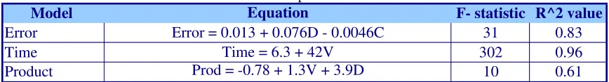
The data analysis results (Table 4) showed that the system is insensitive to the network’s time-delay. The most surprising result was that, even with respect to the run time, a simple linear model involving only the maximum speed of the vehicle was proven to be extremely accurate. Although, these might suggested that for the range of time-delays used the system could be insignificant to the network’s delay we decided to increase the range of this parameter to understand how it would affect the system’s performance when its values become larger.

Table 4 Pilot Experiment’s Results

Model Equation F- statistic R^2 value

Error Error = 0.013 + 0.076D - 0.0046C 31 0.83

Time Time = 6.3 + 42V 302 0.96

Product Prod = -0.78 + 1.3V + 3.9D 10 0.61

Considering the above we decided to modify the ranges for both parameters. The final ranges of variation were set as:

SECTION V: D

ATA

A

NALYSIS AND

D

ISCUSSION

Our goal in this study is to find some estimators, Si* = Hi*(A), of the performance

characteristics, Si = Hi(A). These estimators should provide the information necessary to

draw conclusions about the sensitivity of the system with respect to the studied parameters relevant to each of the performance measures we defined. We planned to extract the functions Hi*(A) using linear regression analysis. To do this, a 34-factorial

experiment was designed and the collected data was processed and analyzed accordingly. In the following sections we provide details of the procedures we followed during the experiments and the data analysis.

5.1

Experimental setup

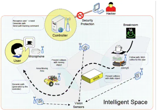
The sensitivity analysis experiments were run in ADAC iSpace (Figure 7). This intelligent space is comprised of four cameras, personal computers with appropriate software and several unmanned ground vehicles. The cameras, the computers and the vehicles are connected together through Ethernet and a wireless network.

(Figure 8) and when it reaches its destination the program terminates, providing measurements of the deviation error and the completion time. These two values are recorded in an Excel spreadsheet and the actual path tracked by the vehicle is plotted in MATLAB (Appendix C).

Figure 7 iSpace in ADAC Lab at NCSU

The procedure is repeated again by placing ANA2 at its initial position and setting the values of the input parameters for the next treatment combination (Table 5).

Figure 8 Different positions of the UGV on the paths

guaranteed, we assume that the actual error for that part of the path will be negligible compared to the deviation error measured for the curved part of path. Therefore, the lengths for each path were calculated as the product of their radius with pi (π_).

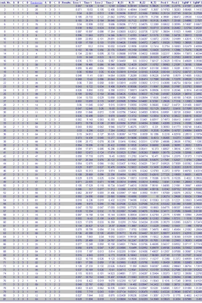
In Table 6, the first five columns populate the 81 different treatment combinations studied and the next five show the actual sequence of treatment combinations used in the experiments. The actual sequence was extracted by randomizing the original one to avoid any systematic errors. The following eight columns show the raw data recorded from the experiments and their normalized values. The following two columns show the values of the product of the normalized error with the normalized time, which will be used to extract the unknown model for the third performance measure of the system. The square root of this product is shown in the last two columns of the table.

5.2

Regression Analysis

Regression analysis is a well-defined simple to conduct and extensively used variance based method for statistical inferences. It involves fitting experimental data on a straight line, when one parameter is involved, on a plane for two parameters and on a “linear” hyper-surface when applied in the multi-dimensional space. The fit is achieved based on least square methodology.

5.2.1 Regression Models for the Deviation Error

Linear Model

As a first approach, the model equation, relating the dependencies between the four parameters of interest and the deviation error, was assumed linear:

tot 0 1 del 2 max 3 max 4

E

= +

b

b

τ

+

b V

+

b D

+

b C

The five unknown coefficients, b0 – b5, were to be estimated from the linear regression of

the independent variables on the error variable. The values used for the error were the average of the two measured values obtained from each of the 81 experimental runs. The significance of each coefficient was determined by inspecting the respective p-value obtained by the analysis. Considering significance level of 0.05, the coefficients whose p-value was higher than 0.05 were assumed insignificant. The least significant factor, denoted by the coefficient with the highest p-value, was then excluded from the model and another regression was run over the remaining factors. The same procedure was repeated until all the remaining factors were significant. The final outcome of the regression suggested the following linear model:

max

0.054 0.028

0.0029

Error

=

−

D

−

C

Full regression model

these terms was run over the measured error values and following the same elimination procedure as above the analysis provided the following model:

del max del max

del max max del max max

0.11 0.23

0.43

0.0089

2.3

4.6

1.4

Error

V

C

V

V

D

V

D

C

τ

τ

τ

τ

=

−

−

−

+

−

−

+

Conceptual model

Finally, a third model was derived based on a more intuitive approach. The error, as explained previously, was expected to increase as the values of the input parameters increase. Assuming a linear relationship, we conclude in eq. 5.2. However, if in addition we assume higher order interactions, then it might be possible to extract some non-linear relations between the deviation error and some of the input parameters. To do that, we first consider the interactions of the path’s curvature with the rest of the parameters. We expect that at high curvature points increased values of either τ_{del, Vmax or Dmax can lead} to higher deviation error. Considering the interactions of the look-ahead distance and either τ_{del or Vmax, we can assume that they will not be significant. These parameters may} independently affect the deviation error, however, we cannot justify a more severe effect due to their combination. On the other hand, the time-delay – speed interaction can be considered significant. Intuitively we can assume that the effect of τ_{del will be more} severe if the speed of the vehicle is higher.

In addition to the above, we wished to include another non-linear term in this model. Observing the effect of Dmax in the linear model we were surprised to see its

and for this reason we filtered a second copy of our data to get more information about the independent effect of the parameters. That analysis suggested a possible second order relation between the deviation error and the look-ahead distance. If we consider a sufficiently small Dmax, then at each iteration, the vehicle will be sent towards a point on

the path close to it. Due to the physical size of the vehicle it might be necessary to loop around itself for some time in order to reach its destination point. This will result in oscillations and thus, increased error. Since high look-ahead distances are expected to also increase the error, an optimal point within the range of variation may exist. According to our data, this point could be close to the value of 0.2m and therefore assuming a quadratic relation between this parameter and the error output may be worth-investigated. We included all the above effects in a regression table and run multiple analyses, dropping each time the least significant factor. We concluded in the following model, which seams to prove our assumption, as the D2max term is one of the most

significant ones:

del max max

2

del max max max

0.15 0.23

0.43

0.47

0.011

2.1

0.040

0.87

Error

V

D

C

V

D

C

D

τ

τ

=

−

−

−

−

+

+

+

+

5.2.2 Regression Models for the Completion Time

Linear model

collected from the experiments and gradually reduced the model based on the parameters’ significance. The following equation corresponds to the best, in the least square sense, linear relationship that can be derived based on the measurements:

del max max

14 35

68

22

1.0

Time

=

+

τ

−

V

−

D

+

C

Full regression model

Considering higher order interactions, as we did for the deviation error model, a completion time model was derived based on full regression of the fifteen possible effects of the four input parameters. Based on a one-at-a-time elimination procedure the resulting full regression model is:

max max del max del max max del max max del max

17 120

19

450

13

230

1400

60

Time

V

D

V

C

V

D

V

D

V

C

τ

τ

τ

τ

= −

−

+

+

+

+

−

−

Conceptual model

An intuitive approach, relating the system’s run time with the four input parameters and their interactions could not be easily developed. In order to see if any important second interactions existed between the parameters, we decided to include all of them in a regression table and run the analysis. Using successive reductions in the model we concluded with the following:

del max del max del max

11 60

67

160

2.5

2.75

Time

V

D

C

D

C

τ

τ

τ

=

+

−

−

+

5.2.3 Regression Models for the Root Error-Time product

Linear model

A linear model was also considered as an initial assumption for the product of the total error and the time to completion. This performance measure provides some information about the trade-off existing between accuracy on tracking and speed on task completion. Regression analysis results provided the following model:

del max max

2.3 1.8

4.2

1.7

0.34

Prod

=

+

τ

−

V

−

D

−

C

Full regression model

As in the case of the first two performance measurements, a full regression model was derived for the error-time product. The elimination procedure resulted in the following model:

max del max max del max max del max del max max

2.8 13

0.53

66

2.4

200

14

49

Prod

V

C

V

V

C

V

D

V

C

V

D

C

τ

τ

τ

τ

=

−

−

+

+

−

−

−

+

Conceptual model

considered τ_del-Vmax, τ_{del-Dmax and Dmax-C interactions in the product model. The} quadratic effect of the look-ahead distance was also included in the table and repeated regression of these effects on the product values resulted in the following model:

max max del max 2

del max max max

3.9 10

11

0.55

33

11

1.1

20

Prod

V

D

C

V

D

D

C

D

τ

τ

=

−

−

−

+

−

−

+

+

5.3

Results and Discussion

In the previous paragraph, three different models were derived for each performance measure. The first was based on the assumption that the four input parameters are linearly related to the system’s output, the second one considered all possible interaction effects and the third one was proposed based on an intuitive approach. It is our goal to select the “best” model for each performance measure and use it as the estimation of Si so that sensitivity values can be extracted for the four input

parameters. We use two criteria to define the “best” model. The first one is the value of the F-statistic provided by the regression analysis. Models with higher F-statistics are considered to be superior to the others. In the case the derived models have similar F-values, our decision is then based on the simplicity of the model.

5.3.1 Models for the Deviation Error

exists while the second model includes many higher order interaction effects that cannot be easily explained or comprehended. Based on the above we define:

1 del max max

2

del max max max

ˆ

_{0.15 0.23}

_0.43

_0.47

_0.011

2.1

0.040

0.87

S

V

D

C

V

D

C

D

τ

τ

=

−

−

−

−

+

+

+

+

to be the estimation of the deviation error of the vehicle.

Table 6 Models for the Deviation Error

Model Error F- statistic R^2 value

Linear Error = 0.054 - 0.028D - 0.0029C 6.8 0.15

Full Regression

Error = 0.11 - 0.23T - 0.43V - 0.0089C + 2.3TV

- 4.6TVD + 1.4TVDC 9 0.42

Conceptual

Error = 0.15 - 0.23T - 0.43V - 0.47D - 0.011C +

2.1TV + 0.040DC + 0.87D^2 13 0.55

According to this equation, the error is a function of all the four input parameters. Applying eq. 3.11 we get:

max del 1 max max

0.23 2.1

0.43 2.1

ˆ

ˆ ( )

0.47 0.04

1.74

0.011 0.04

V

V S

C

D

D

τ

−

+







₋

₊







=



−

+

+





₋

₊





