Exploring Correlation for Indirect Branch Prediction.

(1)

Abstract

PANIRWALA, CHINTAN DIPAKCHANDRA. Exploring correlation for Indirect Branch Prediction. (Under the direction of Dr. Huiyang Zhou.)

History-based branch direction predictors for conditional branches are shown to be highly accurate. Indirect branches however, are hard to predict as they may have multiple targets corresponding to a single indirect branch instruction. With the state of the art predictors like Indirect Target Tagged Geometric length predictor (ITTAGE) which uses long history buffers to predict indirect branches, we still have some branches that are very hard to predict. We observed that in case of some of these branches, the branch target directly depends on the load address which is then used by the branch instruction. Based on this observation we propose Address Target Correlation for prediction of indirect branches.

This work explores two implementations. The first is a hardware only solution and the second is the combined hardware-software solution. In both cases we use ITTAGE as our baseline predictor. In hardware only solution we use a small table termed Address Target Table to predict the targets of hard to predict indirect branches during address generation stage of the load instruction. During the Address Generation (AGEN) stage of load we check if there is some dependent indirect branch and if there is one we provide prediction for that branch. During the execution stage of the indirect branch, we update the address target table based on the actual outcome of the branch. We showed that though hardware only solution is useful, we cannot get much improvements in terms of Misprediction Penalty per Kilo Instruction (MPPKI).

(2)

Exploring Correlation for Indirect Branch Prediction

by

Chintan Dipakchandra Panirwala

A thesis submitted to the Graduate Faculty of North Carolina State University

in partial fulfillment of the requirements for the Degree of

Master of Science

Computer Engineering

Raleigh, North Carolina 2012

APPROVED BY:

____________________________ Dr. Huiyang Zhou

(Committee Chair)

(3)

ii

Dedication

To my beloved parents and sisters

(4)

iii

Biography

(5)

iv

Acknowledgements

First of all, I would like to thank my parents Dipakchandra Panirwala and Rita Panirwala. Through my journey they were a great support and motive for me to succeed. Many thanks to my two twin sisters Hunny and Dimpy for their support.

I would like to have special thanks to my Advisor Prof. Huiyang Zhou. His non-stopping help, attention, and guidance kept me going forward even during the rough times. During my two years at graduate school I learned a lot from him. My grad school journey was not an easy one, but sure after finishing now, I am proud of what we have achieved.

I would like to acknowledge my committee members: Dr. Greg Byrd and Dr. Eric Rotenberg. Thanks for your comments during my defense, they helped to improve the quality of my final thesis.

(6)

v

List of Figures

Figure 1 Indirect Branch Generated by "switch" Statement __________________________ 3 Figure 2 Assembly code for switch-case statement ________________________________ 4 Figure 3 Indirect Branch Generated by Pointer to a Function ________________________ 5 Figure 4 Assembly code for pointer to a function call ______________________________ 6 Figure 5 Indirect Branch Generated by Virtual Function Call ________________________ 7 Figure 6 an entry in ITTAGE predictor ________________________________________ 12 Figure 7 ITTAGE Predictor _________________________________________________ 13 Figure 8 Code example of address-target correlation ______________________________ 15 Figure 9 Address Target Table to exploit ATC __________________________________ 16 Figure 10 Trace for SERVER01 when target = 0x409080 __________________________ 17 Figure 11 Trace for SERVER01 when target = 0x40908f __________________________ 17 Figure 12 MPKI for ITTAGE ________________________________________________ 21 Figure 13 MPPKI for ITTAGE _______________________________________________ 21 Figure 14 Total MPKI for ITTAGE + ATT configuration __________________________ 23 Figure 15 Percentage Improvements in MPPKI for ITTAGE + ATT configuration ______ 24 Figure 16 Comparison of MPKI between ITTAGE and ITTAGE + 8*8 ATT for INT05,

INT06 and SERVER01 benchmarks ______________________________________ 26 Figure 17 Comparison of MPPKI between ITTAGE and ITTAGE + 8*8 ATT for INT05,

(10)

ix

(11)

x

List of Tables

Table 1 Storage Cost for Address Target Table __________________________________ 18 Table 2 MPKI and MPPKI for INT05, INT06 and SERVER01 _____________________ 22 Table 3 Improvements in MPKI after using ATC ________________________________ 23 Table 4 Improvements in MPPKI after using ATC _______________________________ 24 Table 5 ATC results for INT05 benchmark _____________________________________ 25 Table 6 ATC results for INT06 benchmark _____________________________________ 25 Table 7 ATC results for SERVER01 benchmark _________________________________ 25 Table 8 Improvements in MPPKI with Multi-level ATC for different predictor sizes ____ 33 Table 9 Cache Parameters used for PIN Instrumentation ___________________________ 52 Table 10 MPKI for SPEC2006 benchmarks with ITTAGE _________________________ 54 Table 11 Hard to predict branches for omnetpp benchmark _________________________ 55 Table 12 Hard to predict branches for povray benchmark __________________________ 58 Table 13 Hard to predict branches for h264ref benchmark _________________________ 60 Table 14 Cycles saved for branches 0x404750, 0x4048df and 0x40894b with 3-bits

confidence counter ____________________________________________________ 63 Table 15 Cycles saved for branch 0x40324e with 3-bits confidence counter ___________ 64 Table 16 Cycles saved for branches 0x404750, 0x4048df and 0x40894b with 2-bits

confidence counter ____________________________________________________ 65 Table 17 Analysis of branch 0x404750 for 3-bits confidence counter _________________ 66 Table 18 Address target correlation level 2 and 3 for profiling period of 200 million

(12)

1

1 Introduction

Modern superscalar processors use pipelining to overlap the execution of instructions and improve performance. This potential overlap of instructions is called Instruction Level Parallelism (ILP). But the control hazards prevent them from taking advantage of all the available ILP. One of the most used mechanisms to overcome control hazards is the branch prediction. Rather than stalling when a branch is encountered, a pipelined processor uses branch prediction to speculatively fetch and execute instructions along the predicted path. As pipeline deepens and number of instructions issued per cycle increases, the penalty for misprediction increases, as does the benefit of accurate branch prediction.

1.1 Indirect Branch

Control hazards are due to branch instructions. Branches can be classified into conditional or unconditional and direct or indirect branches. In case of conditional branches there are only two possibilities. If it is taken then we jump to the specified target and if it is not taken then we go to next Program Counter (PC). Branch prediction research has shown that for a conditional branch instruction, its direction can be predicted with high accuracy. Branch Target Buffer (BTB) can be used to predict the target. Furthermore, a direct branch has a fixed target encoded in the instruction, thus making conditional or unconditional direct branches easier to predict. Unlike direct branches, indirect branch instructions are hard to predict as they may have multiple targets corresponding to a single indirect branch instruction. Indirect branch has the following format:

(13)

2

This can be interpreted as “jump indirect on the eax register”, which would mean that the next instruction to be executed would be at the address whose value is in register eax. Thus, rather than specifying an address of the next instruction to execute, as in a direct branch, the argument specifies where the address is located [1]. We have focused on indirect branches for the x86-64 instruction set architecture.

1.2 Indirect Branch Code Example

Virtual Function call, function call by a pointer to a function and switch statements are the three major sources of indirect branches.

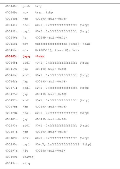
1.2.1 Indirect Branch generated by “switch” statement

(14)

3

Figure 1 Indirect Branch Generated by "switch" Statement

void main (void) {

int ret;

while (1) {

switch (ret) {

case 0:

ret++;

break;

case 1:

ret++;

break;

case 2:

ret++;

break;

case 3:

ret++;

break;

case 4:

ret++;

break;

case 5:

ret++;

break;

default:

ret = 0;

break;

} //end switch

} //end while

(15)

4

400448: push %rbp

400449: mov %rsp, %rbp

40044c: jmp 400490 <main+0x48>

40044e: addl $0x1, 0xfffffffffffffff8 (%rbp)

400452: cmpl $0x5, 0xfffffffffffffffc (%rbp)

400456: ja 400489 <main+0x41>

400458: mov 0xfffffffffffffffc (%rbp), %eax

40045b: mov 0x400598(, %rax, 8), %rax

400463: jmpq *%rax

400465: addl $0x1, 0xfffffffffffffffc (%rbp)

400469: jmp 400490 <main+0x48>

40046b: addl $0x1, 0xfffffffffffffffc (%rbp)

40046f: jmp 400490 <main+0x48>

400475: jmp 400490 <main+0x48>

40047b: jmp 400490 <main+0x48>

40047d: addl $0x1, 0xfffffffffffffffc (%rbp)

400481: jmp 400490 <main+0x48>

400487: jmp 400490 <main+0x48>

400489: movl $0x0, 0xfffffffffffffffc (%rbp)

400490: cmpl $0xc7, 0xfffffffffffffff8 (%rbp)

400497: jle 40044e <main+0x6>

400499: leaveq

40049a: retq

(16)

5

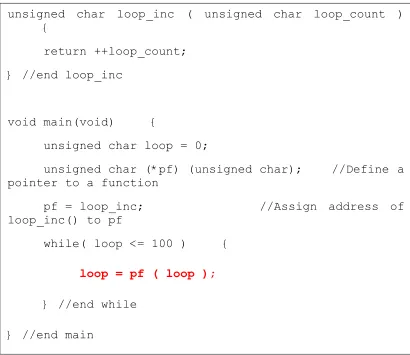
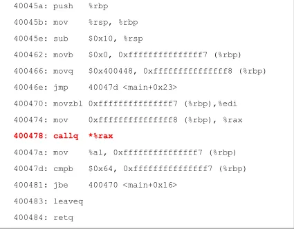
1.2.2 Indirect Branch generated by a pointer to a function

Calling a function pointed by a function pointer will result in an Indirect Branch. Example code is shown in Figure 3. Assembly code for the corresponding example code is shown in Figure 4. Source instruction and mnemonics for Indirect Branch are shown in bold red.

Figure 3 Indirect Branch Generated by Pointer to a Function

unsigned char loop_inc ( unsigned char loop_count ) {

return ++loop_count;

} //end loop_inc

void main(void) {

unsigned char loop = 0;

unsigned char (*pf) (unsigned char); //Define a pointer to a function

pf = loop_inc; //Assign address of

loop_inc() to pf

while( loop <= 100 ) {

loop = pf ( loop );

} //end while

(17)

6

40045a: push %rbp

40045b: mov %rsp, %rbp

40045e: sub $0x10, %rsp

400462: movb $0x0, 0xfffffffffffffff7 (%rbp)

400466: movq $0x400448, 0xfffffffffffffff8 (%rbp)

40046e: jmp 40047d <main+0x23>

400470: movzbl 0xfffffffffffffff7 (%rbp),%edi

400474: mov 0xfffffffffffffff8 (%rbp), %rax

400478: callq *%rax

40047a: mov %al, 0xfffffffffffffff7 (%rbp)

40047d: cmpb $0x64, 0xfffffffffffffff7 (%rbp)

400481: jbe 400470 <main+0x16>

400483: leaveq

400484: retq

(18)

7

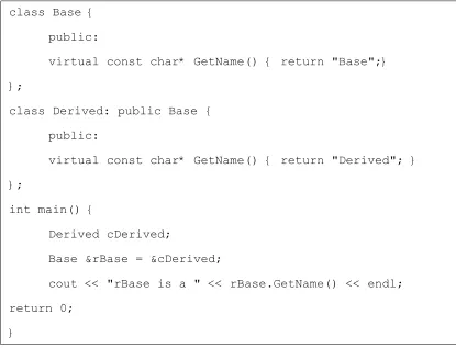
1.2.3 Indirect Branch generated by a Virtual Function call

Object oriented programs are becoming more common as more programs are written in modern high-level languages such as Java, C++ and C#. These languages support polymorphism [2], which signiﬁcantly eases the development and maintenance of large modular software projects. To support polymorphism, modern languages include dynamically dispatched function calls (i.e. virtual functions) whose targets are not known until run-time because they depend on the dynamic type of the object on which the function is called. Virtual function calls are usually implemented using indirect branch/call instructions in the instruction set architecture. Example code for virtual function call is shown in Figure 5.

Figure 5 Indirect Branch Generated by Virtual Function Call class Base {

public:

virtual const char* GetName() { return "Base";}

};

class Derived: public Base {

public:

virtual const char* GetName() { return "Derived"; }

};

int main() {

Derived cDerived;

Base &rBase = &cDerived;

cout << "rBase is a " << rBase.GetName() << endl;

return 0;

(19)

8

1.3 Indirect Branch Prediction

(20)

9

proposed predicting indirect branches via data compression. Their predictor uses the prediction by partial matching (PPM) algorithm of order three, which is a set of four Markov predictors of decreasing size, indexed by an indexing function formed by a decreasing number of bits from previous targets in the target history register. Kim et al. [10] proposed Virtual Prediction Counter (VPC) prediction which uses the existing conditional branch predictor for predicting the indirect branches. Conceptually, VPC treats an indirect branch instruction with number of targets as direct branches, each with its own unique target address. When an indirect jump instruction is fetched, the VPC prediction algorithm accesses the conditional branch predictor for MAXITER times, each time as a different “virtual direct branch’ of the same indirect branch. This iterative process stops either when a “virtual direct branch” is predicted to be taken, or MAXITER number is reached, in which case the processor is stalled until the indirect branch is resolved. Here, MAXITER determines the number of attempts made to predict an indirect branch. Each attempt takes one cycle during which no new instruction is fetched.

(21)

10

directly to the appropriate case block instead of executing a series of conditional branches, the dynamic instruction count is reduced by 9%. However, modern compilers already generate the jump table corresponding to the switch-case statement if the number of cases exceeds certain threshold [5]. If the value of the case variable is not known, CBT redirection is delayed until it is available; resulting in performance degradation for deeply pipelined superscalar processors. Finally, Joao et al. [13] proposed dynamic predication of hard-to-predict indirect jump instructions. When a hard-to-hard-to-predict indirect jump instruction is fetched, the processor starts fetching from N different targets of the jump instruction, thereby increasing the probability of fetching from the correct target path at the expense of executing more instructions. They showed that N=2 is a good trade-off between performance and complexity.

(22)

11

1.3.1 Value Based BTB Indexing

In VBBI for every hard-to-predict static indirect jump instruction, the compiler identifies an instruction whose output value strongly correlates with the target address taken by the jump instruction. When this correlated instruction (hint instruction) produces a value (hint value), the calculated target address of the indirect jump instruction is stored in the BTB at an index computed by hashing the PC of the jump instruction with the hint value. Next time when the jump instruction is fetched, BTB is indexed using its PC and the new hint value to get the predicted target address. In order to maintain strong correlation between the target and the hint value, the current hint value is used. In cases where the latest hint value is not available when the jump instruction is fetched, target prediction is made using old hint value. However, in these cases a second and more accurate target prediction is made using the new hint value when it becomes available. A more accurate second prediction effectively reduces the impact of jump mispredictions on performance by decreasing the jump misprediction penalty.

1.3.2 Compiler Guided Value Pattern

(23)

12

indirect branch instruction is fetched, the predictor uses the hash value of the branch address and the value pattern to get the final predicted target address from the BTB.

1.3.3 ITTAGE

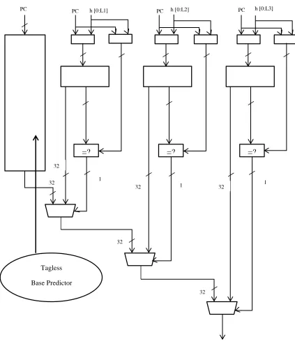
As shown in Figure 7, ITTAGE indexes several predictor tables through independent functions of the global branch/path history and the branch address. A tag-less base predictor provides default prediction. The tagged predictors Ti, 1<i<M, are indexed using history

lengths L (i) = (int) (ai-1 * L (1) + 0.5). History lengths form a geometric series which allows to efficiently capturing correlation on recent branch outcomes as well as on very old branches. A predictor table entry (Figure 6) features target address, a tag, a 2-bit confidence counter “Ctr” allowing some hysteresis on the predictor and a useful bit U for controlling the update policy. At prediction time, the base predictor and the tagged components are accessed simultaneously. The prediction is provided by the hitting tagged predictor component that uses the longest history. In case of no matching tagged predictor component, the default prediction is used. However when the confidence counter of the matching entry is null, the alternate prediction “altpred” is preferred. Generally the predictors tables are updated at retire time to avoid pollution of the predictor by the wrong path. A single predictor table entry may provide several mispredictions in a row due to this late update. In order to reduce this impact, ITTAGE uses the immediate update mimicker (IUM).

Target Tag Ctr U

(24)

13 Tagless

Base Predictor

=? =? =?

PC h [0:L1] PC h [0:L2] PC h [0:L3] PC

Prediction

32

32 32

32

1

1 1

(25)

14

(26)

15

2 Address Target Correlation

2.1 Address Target Correlation Concept

From our trace analysis of the benchmarks, we found that the targets of many hard to predict indirect branches are dependent upon load values. Since the loaded value will be immediately used by the dependent indirect branches, such execution results are available too late to be useful to reduce misprediction penalty. Therefore, we examine the correlation between the producer load addresses and the consumer branch targets, similar to the address-branch correlation observed for conditional branches [17]. Figure shows example code for address-target correlation.

Figure 8 Code example of address-target correlation

From Figure 8, we can see that the producer load accesses two primary addresses and either address contains a different branch target. As long as the data structure (e.g., a virtual function table) at these addresses is not frequently updated, the addresses of the producer loads are sufficient to determine the targets of their consumer indirect branches. We refer to such correlation as address-target correlation (ATC). In our design, we capture ATC in a small cache-like set associative structure, called Address Target Table (ATT) as shown in

Load R19 = Mem [R3] //Address: 0x60848100 0x60846ec8 …

(27)

16

Figure 9. Each entry in ATT contains a tag and multiple pairs of hashed addresses and the corresponding targets.

Figure 9 Address Target Table to exploit ATC

2.1.1 Prediction using ATT

We access the ATT to take a prediction during the Address Generation (AGEN) stage of load instruction. During AGEN stage of a load instruction we check if there is an indirect branch which depends on the load address of this instruction. If we find the correlation, the PC of the consumer indirect branch is used for tag match to see whether an entry in ATT has been allocated for it. If so, the hashed address of the producer load will be used to compare with multiple address-target pairs in the entry to find a matching pair to provide the prediction for the consumer branch. After taking the prediction we compare it with the prediction provided by ITTAGE at fetch stage. If the prediction differs from the one made at the fetch stage of the indirect branch, an early misprediction recovery is initiated to reduce the misprediction penalty.

Hashed Load Address

tag <addr,tar> <addr,tar>

(28)

17

Type Src1 Src2 Src3 Dest Target SRCdata1 SRCdata2 SRCdata3 LDST1 LD_Addr Load 32 2 18 18 0 0 4c4540 1 409080 4c4548

MOV 18 0 0 19 0 409080 0 0 0 0 MOV 30 19 0 19 0 33 409080 0 0 0

JMP 30 19 0 0 409080 33 409080 0 0 0

Figure 10 Trace for SERVER01 when target = 0x409080

Type Src1 Src2 Src3 Dest Target SRCdata1 SRCdata2 SRCdata3 LDST1 LD_Addr Load 32 2 18 18 0 0 4c4540 0 40908f 4c4540

MOV 18 0 0 19 0 40908f 0 0 0 0 MOV 30 19 0 19 0 33 40908f 0 0 0

JMP 30 19 0 0 40908f 33 40908f 0 0 0

Figure 11 Trace for SERVER01 when target = 0x40908f

(29)

18

2.1.2 ATT Update

ATT is updated at the execution stage of an indirect branch. At the execution stage of an indirect branch we check if the branch was mispredicted at the fetch stage. Only if it is mispredicted at the fetch stage, we search for its producer load address and then update ATT with the actual branch target. The least-recently-used (LRU) replacement policy is used to select a victim in ATT. Random replacement is used if there are more address-target pairs than what each entry in ATT can maintain.

2.1.3 Storage Cost

Each entry in address target table contains a tag and multiple address-target pairs. We hash load address and branch PC to compute the tag. We use 32 bits for tag storage. We use 32 bits for storing targets and 10 bits for storing hashed load addresses. Storage requirement for LRU field depends on number of entries (N) in the address target table and is . Storage requirements are shown in Table 1.

Table 1 Storage Cost for Address Target Table

<Number of Entries, Address-Target Pairs> Storage Cost (Bytes)

<26,10> 1485

<8,8> 371

(30)

19

2.2 Evaluating Address Target Correlation

2.2.1 Methodology

For the experiments in this section we used simulation infrastructure provided in Championship Branch Prediction (CBP). The framework models a simple out-of-order core with following parameters.



256-entry reorder buffer, and three schedulers: an integer scheduler with 64 entries and a floating point and load/store schedulers with 32-entries each.



The processor has a 14-stage, 4-wide pipeline except in the execution stage where it has a 12-wide execution scheduler (6 integer, 4 FP and 2 load-store).



The memory model consists of a 2-level cache hierarchy, consisting of an L1 split instruction and data caches, and an L2 last level cache. All caches support 64-byte lines. The L1 instruction cache is 32KB 8-way set associative cache. The L1 data cache is 32KB 8-way associative. The L2 data cache is a 4 MB, 8-way set-associative cache.

(31)

20

the pipeline. We used this information to check for the address-target correlation and how much cycles we can save by correcting the misprediction.

To this infrastructure, we added our modification to detect address target correlation and a small cache like set associative structure to take prediction. We look six instructions back to trace address target prediction. We took prediction in the address generation stage of the load instruction. However, we only took prediction if it was different from the one provided by ITTAGE in fetch stage. We only updated our predictor if there was misprediction in the fetch stage by ITTAGE.

2.2.2 ITTAGE Results

(32)

21

Figure 12 MPKI for ITTAGE

Figure 13 MPPKI for ITTAGE

0 0.5 1 1.5 2 2.5

M

PK

I

Benhcmarks

MPKI

0 50 100 150 200 250 300

M

PP

K

I

(c

yc

le

s)

Benchmarks

(33)

22

Table 2 MPKI and MPPKI for INT05, INT06 and SERVER01

Benchmark MPKI MPPKI

INT05 2.1874 187.99

INT06 2.0773 179.34

SERVER01 1.2663 276.14

Total 5.5310 643.47

2.2.3 ATC Results

We evaluated ATC on the same CBP benchmarks on which results for ITTAGE are shown. We used 64 KB ITTAGE as our baseline predictor which would provide prediction at fetch stage. During AGEN stage, we only take prediction from ATT if its prediction is different from the one provided by ITTAGE at fetch stage. Also during execute stage; we only update ATT if the branch was mispredicted at the fetch stage.

2.2.3.1 MPKI Results

(34)

23

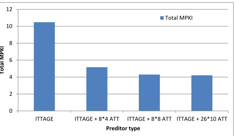
Table 3 Improvements in MPKI after using ATC

Predictor Total MPKI Percentage Improvements

ITTAGE 10.4836 00.00

ITTAGE + 8*4 ATT 5.1664 50.72

ITTAGE + 8*8 ATT 4.2949 59.03

ITTAGE + 26*10 ATT 4.2041 59.89

Figure 14 Total MPKI for ITTAGE + ATT configuration

0 2 4 6 8 10 12

ITTAGE ITTAGE + 8*4 ATT ITTAGE + 8*8 ATT ITTAGE + 26*10 ATT

To

tal M

PK

I

Preditor type

(35)

24

2.2.3.2 MPPKI Results

Table 4 shows percentage improvements we get in MPPKI after using Address Target Correlation at the AGEN stage in co-operation with the ITTAGE at fetch stage. The results were obtained while looking back 6 instructions for address-target correlation.

Figure 15 Percentage Improvements in MPPKI for ITTAGE + ATT configuration

Table 4 Improvements in MPPKI after using ATC

Predictor Total MPPKI Percentage Improvements

ITTAGE 1364.11 _0.00

ITTAGE + 8*4 ATT 1327.96 2.65

ITTAGE + 8*8 ATT 1322.56 3.05

ITTAGE + 26*10 ATT 1321.43 3.11

Early misprediction recovery using ATT with 8 entries and 4 address-target pairs provides a 2.65% improvement in MPPKI compared to ITTAGE. Using ATT with 8 entries and 8 address-target pairs gives an improvement of 3.05%. However, large ATT with 26 entries and 10 address-target pairs does not give much benefit.

2.4 2.5 2.6 2.7 2.8 2.9 3 3.1 3.2

ITTAGE + 8*4 ATT ITTAGE + 8*8 ATT ITTAGE + 26*10 ATT

p

e

rc

e

n

tge

(36)

25

2.2.4 ATC

Results

for

INT05, INT06 and SERVER01

benchmarks

Earlier we observed that for ITTAGE predictor, INT05, INT06 and SERVER01 accounts for about half of the total MPKI and MPPKI of all the CBP benchmarks. The results below show how our predictor fairs on these benchmarks.

Table 5 ATC results for INT05 benchmark

Predictor Coverage (%)

Accuracy (%) Improvements in MPKI (%)

Improvements in MPPKI (%)

ITTAGE+8*4 ATT 84.04 100 84.02 6.07 (11 cycles) ITTAGE+8*8 ATT 99.39 100 99.39 7.17 (13 cycles) ITTAGE+26*10 ATT 99.44 100 99.44 7.18 (13 cycles)

Table 6 ATC results for INT06 benchmark

Table 7 ATC results for SERVER01 benchmark

(37)

26

As shown in Table 5 for INT05 benchmark, 8*4 ATT is able to provide prediction for about 84% of the mispredicted branches with 100 % accuracy which reduces MPKI from 2.1874 to 0.3491 and MPPKI from 187.99 to 176.50. Increasing the predictor size we can achieve almost 100% coverage and as a result MPKI drops to 0.0133.

As shown in Table 6 for INT06 benchmark, 8*4 ATT is able to provide prediction for about 80% of the mispredicted branches with 100 % accuracy which reduces MPKI from 2.0773 to 0.4172 and MPPKI from 179.34 to 169.02. As is the case with INT05 benchmark, increasing predictor size achieves 100% coverage reducing MPKI to 0.0123.

However SERVER01 represents an interesting case where size of the predictor does not make any difference to the performance. As shown in Table 7 Even with 8*4 ATT we can achieve 100% coverage which reduces MPKI from 1.2663 to 0.0077 and MPPKI from 276.14 to 265.98.

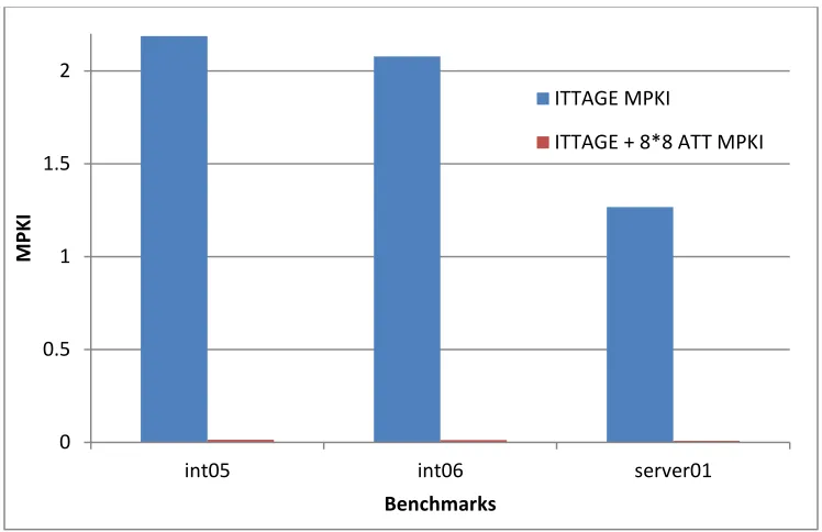
Figure 16 Comparison of MPKI between ITTAGE and ITTAGE + 8*8 ATT for INT05, INT06 and SERVER01 benchmarks

0 0.5 1 1.5 2

int05 int06 server01

M

PK

I

Benchmarks

ITTAGE MPKI

(38)

27

This may be due to the fact that SERVER01 has a very few hard to predict branches with a very few disparate targets. But these branches occur highly frequently and are so random in behavior that ITTAGE is not able to capture the history information properly.

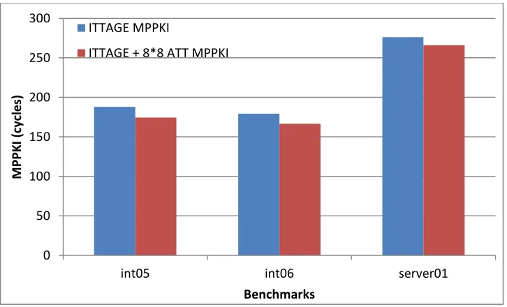
As shown in Figure 16, by using 8*8 ATT at the AGEN stage to exploit address target correlation while looking back for 6 instructions with ITTAGE as main predictor we are able to bring down MPKI to almost zero for these three benchmarks. Figure 17 shows that Address-target correlation is able to achieve on average reduction of 11 cycles for these three benchmarks. This relatively limited performance enhancement is due to the fact that the latency between the AGEN stage of a producer load and the execution (EXE) stage of its consumer indirect branch is often a small portion of the misprediction penalty, which starts from the fetch stage of the indirect branch. For higher performance gains we need to explore address-target correlation beyond the immediate producer-consumer pairs.

Figure 17 Comparison of MPPKI between ITTAGE and ITTAGE + 8*8 ATT for INT05, INT06 and SERVER01 benchmarks

0 50 100 150 200 250 300

int05 int06 server01

M

PP

K

I

(c

yc

le

s)

Benchmarks ITTAGE MPPKI

(39)

28

3 Multi-Level Address Target Correlation

In previous chapter, we concluded that using one level of address-target correlation and looking at immediate load address to predict indirect branch outcome does reduce MPKI to almost zero but it does not give much improvements in terms of MPPKI. This phenomenon is shown in Figure 18. As shown in Figure 18, indirect branch is fetched at cycle 3734276 and is resolved in execution stage at 3734362. Thus if this branch was mispredicted, it will incur a penalty of 86 cycles. However with address-target correlation we can accurately predict the branch outcome during the address generation stage of the load instruction. In this case also we will not be able to predict target before cycle 3734356 which is just 6 cycles before the indirect branch finally gets resolved in execution stage.

Type src1 src2 src3 dst Target srcval1 srcval2 srcval3 ld_addr

fetch cycle

execute cycle

Load 32 2 18 18 0 0 4c4540 1 4c4548 3734275 3734356 MOV 18 0 0 19 0 409080 0 0 0 3734276 3734358 MOV 30 19 0 19 0 33 409080 0 0 3734276 3734360 JMP 30 19 0 0 409080 33 409080 0 0 3734276 3734362

Figure 18 MPPKI gain for immediate Address Target Correlation

(40)

29

3.1 Multi-Level Address Target Correlation Concept

As shown previously, looking at immediate load instruction for address-target correlation does not give much benefit in terms of MPPKI as the branch is resolved too late in the pipeline stage. However if we can find address target correlation beyond the immediate load instruction we may be able to get more benefits in terms of MPPKI. This gives motivation for the multi-level Address Target Correlation.

3.1.1 First Level of Address-Target Correlation

Figure 19 Instruction trace for First Level of ATC

As explained previously, we only look for correlation between load address and immediate indirect branch. In Figure 19, there is an address-target correlation between Load* R19 and

Load R3 = Mem[R2 + …]

Mov R9 = R3

…

Load*R19 = Mem[R3 + …]//LoadAddress:60848100 60846ec8

…

(41)

30

Indirect branch R19 instruction. Load instruction always reads from two different addresses which results in two different targets. There is very high probability that this relationship will be one-to-one and we will be able to predict branch target accurately. However Load* and indirect branch may not be apart by more than 5-10 cycles and hence there is not much benefit in terms of MPPKI.

3.1.2 Second Level of Address-Target Correlation

Figure 20 Instruction trace for Second Level of ATC

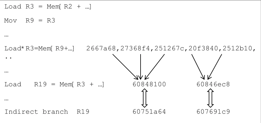
In Figure 20, we have address-target correlation between immediate load-indirect branch pair. But looking beyond we find that the Load R19 gets its address form the Load* R3 instruction. Load R3* reads from multiple addresses and based on that address, the Load R19 will get the address from which it will be reading. We can also see that in this example there is many-to-one relationship which is still useful for accurately predicting branch target. In

Mov R9 = R3

…

Load*R3=Mem[R9+…] 2667a68,27368f4,251267c,20f3840,2512b10, ..

…

Load R19 = Mem[R3 + …] 60848100 60846ec8

…

(42)

31

this case Load* instruction may be 10-20 cycles away from consumer branch instruction and hence if we can accurately predict branch target from this load address we can get more benefit compared to the first case. Also we may start observing many-to-one, many-to-many or one-to-many relationship at this level. Many-to-many or one-to-many relationships are not useful for branch prediction.

3.1.3 Third Level of Address-Target Correlation

Figure 21 Instruction trace for Third Level of ATC

In Figure 21, we are looking beyond second level. At this level we see that Load* R3 provides values for address calculation for second level load. At this level Load* instruction may be 30-50 cycles apart and thus if we can use this load address to predict branch target, we may be able to get more performance benefit in terms of MPPKI. However, as we go away from the indirect branch for tracing address-target correlation we may not get one-to-one or many-to-one-to-one relationships which are required for accurate prediction.

Load*R3=Mem[R2 + …] 0,1,2,3,4,5,6,…(offset to base)

Mov R9 = R3

…

Load R3 =Mem [R9+…]2667a68,27368f4,251267c,20f3840,2512b10

…

Load R19 = Mem[R3 + …] 60848100 60846ec8

…

(43)

32

3.2 Evaluating Multi-Level Address Target Correlation

We evaluated multi-level address target correlation for INT05, INT06 and SERVER01 benchmarks from CBP benchmarks. We observed that for INT05 and INT06 benchmarks, there is no address target correlation beyond immediate level. However SERVER01 benchmark has the potential for multi-level address target correlation.

PC Type src1 src2 src3 src4 dst Target LDST1 ld_addr

fetch cycle

execute cycle 408fcf Load 32 2 0 18 14 0 2 5e5544 3734271 3734345 408fd7 MOV 14 0 0 0 13 0 0 0 3734271 3734347 408fda MOV 13 16 0 0 13 0 0 0 3734271 3734349 408fdd LOAD 32 2 17 0 19 0 adf49353 4da464c0 3734272 3734323 408fdf MOV 13 19 0 0 19 0 0 0 3734272 3734351 408fe1 CB 95 30 2 0 0 408ff8 0 0 3734272 3734353 408ff8 Load 32 2 0 18 19 0 1 5e5944 3734273 3734345 408ffc MOV 19 0 0 0 13 0 0 0 3734273 3734347 409000 MOV 14 0 0 0 18 0 0 0 3734273 3734347 409003 MOV 18 2 0 0 18 0 0 0 3734273 3734349 409007 MOV 18 2 0 0 19 0 0 0 3734274 3734351 40900b CB 95 30 2 0 0 4090a0 0 0 3734274 3734354 409014 Load 32 2 0 18 19 0 409080 4c4548 3734275 3734356 40901e JMP 30 19 0 0 0 409080 0 0 3734276 3734362

Figure 22 Instruction trace for SERVER01 benchmark

(44)

33

Now source register of this MOV gets its value from MOV at 0x409000. Source register of this MOV is the destination register of load instruction at 0x408fcf. Now we found that there is many-to-one correlation between load address of this instruction and target of the indirect branch at 0x40901e. Hence we can use the address of this load to predict the outcome of the indirect branch. Since this address will be available in the address generation stage of the load instruction at 0x408fcf, we can make a prediction at cycle 3734345. Now indirect branch at 0x40901e will get resolved in execution stage at cycle 3734362. As a result we can save almost 17 cycles in this case. As shown in Figure 23, this gives overall improvement of about 16 cycles for SERVER01 benchmark with 8*8 ATT.

Table 8 Improvements in MPPKI with Multi-level ATC for different predictor sizes

Predictor MPPKI improvement with

Immediate ATC

MPPKI improvement with Multi-level ATC

ITTAGE + 8*4 ATT 3.68% (10 cycles) 4.48% (12 cycles) ITTAGE + 8*8 ATT 3.68% (10 cycles) 5.70% (16 cycles) ITTAGE + 26*10 ATT 3.68% (10 cycles) 5.70% (16 cycles)

Figure 23 Improvements in MPPKI for Multi-level ATC

250 255 260 265 270 275 280

ITTAGE ITTAGE + Immediate ATC ITTAGE + Multilevel ATC

(45)

34

(46)

35

4 Compiler Assisted Address Target

Correlation

Thus address-target correlation beyond immediate level has significant potential for performance improvement. We may be able to get more benefits if we can look further for the addresses that can give us hint about the outcome of the current indirect branch. Such correlation can be easily and effectively identified by the compiler based on high level dataflow information. Based on this observation, we argue that a compiler-microarchitecture co-operative approach can be more accurate and more efficient to trace address target correlation. Recent research [15] has shown value correlation is more effective than traditional history correlation for indirect branch prediction. However, there is a limitation for the value correlation in that it is very difficult to find proper data values that have strong correlation with branch targets. Previous predictors generally rely on large storage buffer [18], complex control logics [19] or expensive manual profiling [15] to identify proper value correlation, and they are usually ineffective even with aggressive hardware support. However, we propose to identify effective address target correlation based on high level dataflow information at compile time.

(47)

36

4.1 Instrumentation

4.1.1 Instruction trace analysis

After analyzing branch prediction behavior of ITTAGE for each benchmark, we have a list of indirect branches with a very high dynamic count and are very hard to predict. For these hard to predict indirect branches we generated instruction trace containing information such as program counter, opcode, source registers and their values, destination register and their values, if the instruction is load or store, load or store addresses and if there was a hit or a miss in I-cache or D-cache for this instruction. We used information from this dynamic instruction trace to get the understanding of the code that generates hard to predict branches. We also used the same instruction trace to track address target correlation between producer load addresses and consumer indirect branch. We also analyzed if there is one-to-one, many-to-one or one-to-many relationships between producer load address and consumer indirect branch. Section below shows code behavior of some of the hard to predict indirect branches.

4.1.1.1 Indirect Branch 0x404750

(48)

37

Thus there is address target correlation between load addresses for “pieces [j]’ and the target of the indirect branch 0x404750.

Figure 24 Source code for indirect branch 0x404750

4.1.1.2 Indirect Branch 0x40894b

Figure 26 shows a source code for the indirect branch 0x40894b which is example of the indirect branch generated by a pointer to function call. The branch has a dynamic count of 263142805 and has a misprediction rate of 4.6%. Different function pointer will be called based on the return value of function “piecet (i)”. Variable ‘i’ gets its value from “pieces[j]”.

if (white_to_move) {

for (a = 1, j = 1; (a <= piece_count) &&

(((Variant != Suicide) && ! kingcap) ||

((Variant == Suicide) &&

(fcaptures == captures))); j++) {

i = pieces[j];

if (! i)

continue;

else

a++;

from = i;

gfrom = i;

switch (board[from]) {

(49)

38

(50)

39

4046de: mov 4758268(%rip), %eax #88e1e0 <white_to_move>

4046e4: test %eax, %eax

4046e6: je 40487b <gen+0x1cb>

4046ec: mov 4767354(%rip), %eax # 89056c <piece_count>

4046f2: xor %ebp, %ebp

4046f4: mov $0x1, %r13d

4046fa: test %eax, %eax

4046fc: jle 404822 <gen+0x172>

404702: mov 4759496(%rip), %ecx # 88e6d0 <Variant>

404708: $0x3, %ecx

40470b: je 404ba8 <gen+0x4f8>

404711: mov 2314921(%rip), %eax # 6399c0 <kingcap>

404717: test %eax, %eax

404719: jne 404822 <gen+0x172>

40471f: mov 0x890b64 (, %rbp, 4), %ebx

404726: test %ebx, %ebx

404728: je 404811 <gen+0x161>

40472e: movslq %ebx, %rdx

404731: add $0x1, %r13d

404735: mov %ebx, 2314893(%rip) # 6399c8 <gfrom>

40473b: cmpl $0xb, 0x875bc0 (, %rdx, 4)

404743: ja 404811 <gen+0x161>

404749: mov 0x875bc0 (, %rdx, 4), %eax

404750: jmpq *0x419f20 (, %rax, 8)

(51)

40

for (j = 1, a = 1; (a <= piece_count); j++) {

i = pieces[j];

if (! i)

continue;

else

a++;

score+= (*(evalRoutines[piecet(i]))(i,pieceside(i));

408915: add $0x1, %rbp

408919: cmp 4750412(%rip),%r12d # 89056c <piece_count>

408920: jg 4090f9 <std_eval+0xaa9>

408926: mov 0x890b64 (, %rbp, 4),%edi

40892d: test %edi, %edi

40892f: je 408915 <std_eval+0x2c5>

408931: movslq %edi, %rbx

408934: add $0x1, %r12d

408938: mov 0x875bc0 (, %rbx, 4), %esi

40893f: add $0x1, %esi

408942: mov %esi, %eax

408944: and $0x1, %esi

408947: sar %eax

408949: cltq

40894b: callq *0x41a320 (, %rax, 8)

(52)

41

4.2 Algorithm

Usually target of indirect branch is written to the register via some load instruction. If there is one to one or many to one correlation between this producer load instruction and consumer indirect branch we can exploit it to accurately predict the outcome of the branch instruction. The earlier in the dynamic instruction trace we identify such load instructions, the more benefits we can get in terms of MPPKI savings. We have developed such compiler algorithm that traces the address target correlation in the dynamic instruction trace and tries to correct the target prediction of indirect branch that was mispredicted by ITTAGE. The algorithm also tries to predict the address target correlation level from which to take a prediction based on one-to-one, many-to-one or one-to-many relationships that exist at that level between producer load addresses and consumer indirect branch.

4.2.1 Algorithm to trace address target correlation

The key steps in tracing algorithm are as followed:

 Fill in the instruction queue and start tracing algorithm if the last instruction is hard to predict indirect branch.

 Check if the source registers of the instruction pointed by cnt1 matches with the destination register of the instruction pointed by cnt2.

 If there is a match, use the source registers or the load address of the instruction pointed by cnt2 for prediction.

(53)

42

(54)

43

Figure 28 Algorithm to trace Address Target Correlation

set queue_size;

Fill in the instruction queue

If(current_instruction==hard_to_predict_indirect_branch) {

set cnt1 to queue_size – 1;

for (cnt2 = cnt1 – 1;cnt2 >= stop_level;) {

if(instruction[cnt1].src==instruction[cnt2].dst)

{

prediction_src = instruction[cnt2].src ;

set match1;

set match2;

}

decrement cnt2;

if match2 is set

cnt1 = cnt2;

else

cnt1 = cnt1;

}

if match1 is set

take prediction;

update predictor based on actual branch outcome;

(55)

44

4.2.2 Algorithm to determine stop_level

The key steps in stopping algorithm are as followed:

 Maintain a load table where each entry is the load address and the branch targets it points to. We maintain this information for each level of correlation.

 Check if at particular correlation level, there is one-to-one or many-to-one correlation between load address and branch targets.

 We start checking this information from the farthest level. If we find that there is one-to-many or many-one-to-many relation, we do not take prediction from that level and we come down one level.

 We repeat above steps till we find appropriate level where we can get one-to-one or many-to-one relations.

(56)

45

(57)

46

Figure 29 Algorithm to detect stop_level

set queue_size; Fill in the instruction queue;

if(current_instruction==hard_to_predict_indirect_branch) {

set stop_level = 1;

for (i = 0; i < queue_size; i++) {

if (ld_table[i].load_address.size() < 2 &&

ld_table[i].load_address.size() != 0)

stop_level = level[i];

}

set cnt1 to queue_size – 1;

cnt3 = 0;

for (cnt2 = cnt1 – 1; cnt2 >= stop_level;) {

if(instruction[cnt1].src==instruction[cnt2].dst) {

pred_src = instruction [cnt2].src;

level[cnt3] = cnt2;

ld_table[cnt3].load_address[pred_src].puch_back (target);

set match1; set match2;

cnt3++;

}

decrement cnt2;

if match2 is set

cnt1 = cnt2;

else

cnt1 = cnt1;

}

if match1 is set

take prediction;

update predictor based on actual branch outcome;

(58)

47

4.3 Case Study

PC

OPCODE

Source

Value Dest. Dest Value

Load Address

404a8c ADD rbp 1 rbp 2 0

404a90 CMP r13d 3 rflags 297 89056c

404702 MOV 0 0 rcx 2 88e6d0

404708 CMP rcx 2 rflags 297 0

40470b JZ rip 40470b rip 404711 0

404711 MOV 0 0 rax 0 6399c0

404717 TEST rax 0 rflags 246 0 404719 JNZ rip 404719 rip 40471f 0

40471f MOV rbp 2 rbx 26 890b6c

404726 TEST rbx 26 rflags 202 0 404728 JZ rip 404728 rip 40472e 0

40472e MOVSXD rbx 26 rdx 26 0

404731 ADD r13d 3 rflags 4 0

404735 MOV rbx 26 rip 0 0

40473b CMP rdx 26 rflags 297 875c58 404743 JNBE rip 404743 rip 404749 0

404749 MOV rdx 26 rax 1 875c58

404750 JMP rax 1 rip 0 419f28

(59)

48

(60)

49

Back trace level 0

Load Address Target

875c30 404757 875c34 404a33 875c58 4048e6 875c5c 4048e6

875c60 4048e6 404811 404757 875c74 4048e6

875c8c 404811 404aa2 875c90 404811

875ca0 404aa2 875ca4 404b66

Back Trace Level 2 Back Trace Level 3

Load Address Target _{Source value} _Target

890b64 404757 ₀ _404a33

890b68 404a33 ₁ _4048e6

890b6c 4048e6 ₂ _4048e6

890b70 4048e6 ₃ _4048e6

890b74 4048e6 ₄ _4048e6

890b78 4048e6 ₅ _404aa2

890b7c 404aa2 ₆ _404b66

890b80 404b66 ₇ ₄₀₄₈₁₁

890b84 404811 ₈ _4048e6

890b88 4048e6 ₉ ₄₀₄₈₁₁

890b8c 404811 _a ₄₀₄₈₁₁

890b90 404811 _b ₄₀₄₈₁₁

890b94 404811 _c _4048e6

890b98 4048e6 _e ₄₀₄₈₁₁

890ba0 404811 _f ₄₀₄₈₁₁

890ba4 404811 ₁₀ _404a33

890ba8 404a33 ₁₁ ₄₀₄₈₁₁

890bac 404811 ₁₂ ₄₀₄₈₁₁

890bb0 404811 ₁₄ ₄₀₄₈₁₁

Figure 31 Address target correlation at each level

Back Trace Level 1

Source value Target

1c 404757 1d 404a33 26 4048e6 27 4048e6

28 4048e6 404811 404757 2d 4048e6

33 404811 404aa2 34 404811

(61)

50

As shown in Figure 31, at back trace level zero load address 0x875c30 only points to target 0x404757. However, load address 0x875c60 points to multiple targets. So is the case with load address 0x875c8c. Hence there exists one-to-many relationship at this level. Similarly at back trace level 1, there are one-to-many relationships between some of the source values and branch targets. However, at back trace level 2 there is one-to-one relationship between produce load address and consumer branch targets and we can accurately predict branch outcome from this level. Same is the case with back trace level 3, where there is one-to-one relationship between source values and branch targets.

(62)

51

5 Evaluating Compiler Assisted ATC

5.1 Methodology

For the experiments in this section we used SPEC2006 benchmarks. We used PIN tool from Intel for instrumentation. Pin is a dynamic binary instrumentation framework for the IA-32 and x86-64 instruction-set architectures that enables the creation of dynamic program analysis tools. We used PIN:

 To get the branch prediction results for SPEC2006 benchmarks using 64KB ITTAGE as an indirect branch predictor. We used these results to identify hard to predict branches.

 To generate the instruction trace for the given benchmark binary so that we can trace address target correlation using our algorithm.

 To get the final branch prediction results for SPEC2006 benchmarks using 64 KB ITTAGE with Address Target Table as an indirect branch Predictor.

(63)

52

to get the understanding of the code that generates hard to predict branches. We also used the same instruction trace to track address target correlation between producer load addresses and consumer indirect branch. We also analyzed if there is to-one, many-to-one or one-to-many relationships between produce load address and consumer indirect branch.

Table 9 Cache Parameters used for PIN Instrumentation

L1 Instruction Cache

Cache Size 32 KB

Block Size 64

Associativity 2 Access Time 2 cycles

L1 Data Cache

Cache Size 32 KB

Block Size 64

Associativity 2 Access Time 2 cycles

Unified L2 Cache

Cache Size 2 MB

Block Size 64

Associativity 1

Access Time 10 cycles

Unified L3 Cache

Cache Size 16 MB

Block Size 64

Associativity 1

(64)

53

5.2 ITTAGE MPKI results and analysis

We replaced the default BTB predictor provided by the PIN tool with 64 KB ITTAGE predictor. We collected following data for SPEC2006 benchmarks:

 Total dynamic count of each indirect branch  Misprediction count for that benchmark  MPKI for that benchmark

Figure 32 shows benchmarks with highest MPKI with ITTAGE indirect predictor. MPKI for all benchmarks is shown in Table 10. There is some interesting behavior seen with some of the benchmarks.

 As shown in Table 10, gamess benchmark has the highest MPKI. However the benchmark has a very low dynamic count of indirect branch and even if we predict each branch correctly, there is not much scope for performance improvement.

 Sjeng benchmark has the second highest MPKI. Also it has a very high dynamic count of indirect branch and many of these branches are hard to predict. So it offers good opportunity for performance improvement. Same is the case with dealII, omnetpp, povray, gobmk and h264ref benchmarks.

 MPKI of benchmarks hmmer and xalanc is not as high but there are some hard to predict indirect branches with high dynamic count.

 Lbm and calculix benchmarks have relatively high MPKI but there are not any hard to predict indirect branch with high dynamic count and hence they do not offer much opportunity for performance improvement.

(65)

54

 Benchmarks gromacs, astar, gems, mcf, zeusmp, milc, namd, leslie and bwaves all have very low MPKI and do not offer any opportunity for performance improvement.

Figure 32 most hard to predict benchmarks for ITTAGE

Table 10 MPKI for SPEC2006 benchmarks with ITTAGE

Benchmark MPKI Benchmark MPKI

gamess 0.557434 soplex 8.32E-05 sjeng 0.254975 bzip 5.16E-05 dealII 0.0584253 gromacs 4.15E-06 omnetpp 0.0175544 astar 9.60E-07 povray 0.0170141 gems 4.49E-07 gobmk 0.0150332 mcf 4.04E-07 h264ref 0.00534244 zeusmp 2.57E-07 hmmer 0.00394453 milc 2.38E-07 xalanc 0.00145833 namd 2.16E-07 lbm 0.000278143 leslie 1.72E-07 calculix 0.000177632 bwaves 9.53E-08

0 0.05 0.1 0.15 0.2 0.25 0.3

sjeng dealII omnetpp povray gobmk h264ref hmmer xalanc calculix

M

PK

I

(66)

55

5.3 Benchmark Analysis

Though benchmarks dealII, omnetpp, povray and gobmk have high MPKI and some branches with very high misprediction rate, these branches do not exhibit address target correlation. Some of these branches are explained with code examples in the following sections. Benchmark sjeng has highest MPKI and many of its hard to predict branches exhibit address target correlation.

5.3.1 Omnetpp

Some of the hard to predict branches for omnetpp benchmark are as shown in Table 11. These branches have been classified as hard to predict based on their high misprediction count or high misprediction rate.

Table 11 Hard to predict branches for omnetpp benchmark

Branch PC Dynamic Count Misprediction Count

0x4057cb 3194694 97442

0x40e9e6 520435368 6070981

0x40f7a4 2574274 80384

0x410e9a 150937466 225799

0x45b9e6 276949108 3298492

(67)

56

5.3.1.1 Indirect Branch 0x40e9e6

Figure 33 shows source code for branch 0x40e9e6 and the corresponding assembly code are shown in Figure 34. In address target correlation we look for the correlation between producer load addresses and consumer indirect branches. However, in this case the outcome of the “switch” statement depends on the value of the variable “receiveState” which will be given that value somewhere in the code. So this is the concept used by Value Based BTB Indexing for indirect branch prediction as explained in 1.3.1 and not the address target correlation.

void EtherMAC::printState()

{

#define CASE(x) case x: EV << #x; break

EV << ", receiveState: ";

switch (receiveState) {

CASE (RX_IDLE_STATE);

CASE (RECEIVING_STATE);

CASE (RX_COLLISION_STATE);

}

EV << ", backoffs: " << backoffs << endl;

#undef CASE

}

(68)

57

5.3.2 Povray

Some of the hard to predict branches for povray benchmark are as shown in Table 12. These branches have been classified as hard to predict based on their high misprediction count or high misprediction rate. As mentioned earlier, these branches do not exhibit address target correlation. This phenomenon is explained using one of the branches with its corresponding source code and assembly code in the next subsection.

40e9c0: push %rbp

40e9c1: mov %rdi, %rbp

40e9c4: push %rbx

40e9c5: sub $0x8, %rsp

40e9c9: mov 2674041(%rip), %eax # 69b748 <ev +0x8>

40e9cf: test %eax, %eax

40e9d1: je 40ea80 <EtherMAC::printState () + 0xc0>

40e9d7: cmpl $0x6, 0x2cc (%rbp)

40e9de: ja 40ea08 <EtherMAC::printState () + 0x48>

40e9e0: mov 0x2cc (%rbp), %eax

40e9e6: jmpq *0x46d458(, %rax, 8)

(69)

58

Table 12 Hard to predict branches for povray benchmark

Branch PC Total Dynamic Count Misprediction Count

0x411dc1 4136427432 4082519

0x442d52 18227834 1385094

0x45654e 2186191999 5871880

0x4566d5 514757454 5154863

0x4735aa 30703314 487893

5.3.2.1 Indirect Branch 0x4735aa

Figure 35 shows source code for branch 0x40e9e6 and the corresponding assembly code is shown in Figure 36. In address target correlation we look for the correlation between producer load addresses and consumer indirect branches. However, in this case the outcome of the “switch” statement depends on the value of the variable “Type” which will be given that value somewhere in the code. So this is the concept used by Value Based BTB Indexing

DBL Evaluate_TPat (TPATTERN *TPat, VECTOR EPoint, INTERSECTION *Isection)

{

switch (TPat->Type)

{

case AGATE_PATTERN: value = agate_pattern (EPoint, TPat); break;

...

}

(70)

59

For indirect branch prediction as explained in 1.3.1 and not the address target correlation.

473570: mov %rbp, 0xffffffffffffffd8 (%rsp)

473575: mov %r12, 0xffffffffffffffe0 (%rsp)

47357a: mov %rsi, %rbp

47357d: mov %rbx, 0xffffffffffffffd0 (%rsp)

473582: mov %r13, 0xffffffffffffffe8 (%rsp)

473587: mov %rdi, %r12

47358a: mov %r14, 0xfffffffffffffff0 (%rsp)

47358f: mov %r15, 0xfffffffffffffff8 (%rsp)

473594: sub $0x288, %rsp

47359b: movzwl (%rdi), %eax

47359e: sub $0x5, %eax

4735a1: cmp $0x2d, %ax

4735a5: ja 4735b1

4735a7: movzwl %ax, %eax

4735aa: jmpq *0x4d0a28 (, %rax, 8)

(71)

60

5.3.3 H264ref

Some of the hard to predict branches for h264ref benchmark are as shown in Table 13. The branch has been classified as hard to predict based on its high misprediction count. As mentioned earlier, this branch does not exhibit address target correlation. This phenomenon is explained using corresponding source code and assembly code in the next subsection.

Table 13 Hard to predict branches for h264ref benchmark

Branch PC Total Dynamic Count Misprediction Count

0x43fa34 1975097520 2524634

5.3.3.1 Indirect Branch 0x43fa34

orgptr = orig_blocks;

bindex = 0;

for (blky = 0; blky < 4; blky++)

{

LineSadBlk0=LineSadBlk1=LineSadBlk2=LineSadBlk3 = 0;

for (y = 0; y < 4; y++)

{

refptr = PelYline_11 (ref_pic, abs_y++, abs_x, img_height, img_width);

(72)

61

Figure 37 shows source code for branch 0x43fa34 and the corresponding assembly code is shown in Figure 38. In address target correlation we look for the correlation between producer load addresses and consumer indirect branches. However, we were not able to find any such correlation for this branch. We were also not able to find particular program statement which causes this branch to behave this way.

From above analysis it is clear that benchmarks omnetpp, povray, h264ref and gobmk do not get benefits from address target correlation. The benchmark that benefits most from address target correlation is sjeng. So we present the results for the sjeng benchmark in the following section.

43fa11: mov %r9, 0x30 (%rsp)

43fa16: mov %r10, 0x28 (%rsp)

43fa1b: mov %r11d, 0x20 (%rsp)

43fa20: mov %eax, 0x9c (%rsp)

43fa27: mov 0x54(%rsp), %r8d

43fa2c: mov 0x88(%rsp), %rdi

43fa34: callq *2362742(%rip) # 6807b0 <PelYline_11>

(73)

62

5.4 Performance of Address Target Correlation

Figure 39 Cycles saved for branches 0x404750 and 0x4048df

Figure 40 Cycles saved for branch 0x40894b

Exploring Correlation for Indirect Branch Prediction.

Abstract

Dedication

Biography

Acknowledgements

Table of Contents

List of Figures

List of Tables

1

Introduction

1.1

Indirect Branch

1.2

Indirect Branch Code Example

1.2.1

Indirect Branch generated by “switch” statement

1.2.2

Indirect Branch generated by a pointer to a function

1.2.3

Indirect Branch generated by a Virtual Function call

1.3

Indirect Branch Prediction

1.3.1

Value Based BTB Indexing

1.3.2

Compiler Guided Value Pattern

1.3.3

ITTAGE

2

Address Target Correlation

2.1

Address Target Correlation Concept

2.1.1

Prediction using ATT

2.1.2

ATT Update

2.1.3

Storage Cost

2.2

Evaluating Address Target Correlation

2.2.1

Methodology







2.2.2

ITTAGE Results

2.2.3

ATC Results

2.2.3.1

MPKI Results

2.2.3.2

MPPKI Results

2.2.4

ATC

Results

for

INT05, INT06 and SERVER01

benchmarks

3

Multi-Level Address Target Correlation

3.1

Multi-Level Address Target Correlation Concept

3.1.1

First Level of Address-Target Correlation

3.1.2

Second Level of Address-Target Correlation

3.1.3

Third Level of Address-Target Correlation

3.2

Evaluating Multi-Level Address Target Correlation

4

Compiler Assisted Address Target

Correlation

4.1

Instrumentation

4.1.1

Instruction trace analysis

4.1.1.1

Indirect Branch 0x404750