Scholarship at UWindsor
Scholarship at UWindsor
Electronic Theses and Dissertations Theses, Dissertations, and Major Papers
2011
Time-dependent pointer states, determination of the preferred
Time-dependent pointer states, determination of the preferred
basis of measurement, and decoherence of quantum systems
basis of measurement, and decoherence of quantum systems
Hoofar Daneshvar University of Windsor
Follow this and additional works at: https://scholar.uwindsor.ca/etd
Recommended Citation Recommended Citation
Daneshvar, Hoofar, "Time-dependent pointer states, determination of the preferred basis of measurement, and decoherence of quantum systems" (2011). Electronic Theses and Dissertations. 471.
https://scholar.uwindsor.ca/etd/471
the preferred basis of measurement, and
decoherence of quantum systems
by
Hoofar Daneshvar
A Dissertation
Submitted to the Faculty of Graduate Studies through the Department of Physics in Partial Fulfillment of the Requirements for the Degree of Doctor of Philosophy at the
University of Windsor
by
Hoofar Daneshvar
University of Windsor
This dissertation includes 3 original papers that have been previously submitted for publi-cation in peer reviewed journals, as follows1:
Thesis Chapter Publication title/full citation Publication status
3 Submitted toAnnals of Physics Under Review 4 Submitted toJournal of Physics A Under Review 5 Submitted toJournal of Physics A Under Review
I certify that the above material describes work completed during my registration as grad-uate student at the University of Windsor. I declare that, to the best of my knowledge, my thesis does not infringe upon anyone’s copyright nor violate any proprietary rights and that any ideas, techniques, quotations, or any other material from the work of other people included in my thesis, published or otherwise, are fully acknowledged in accordance with the standard referencing practices. I declare that this is a true copy of my thesis, including any final revisions, as approved by my thesis committee and the Graduate Studies office, and that this thesis has not been submitted for a higher degree to any other University or Institution.
1
We present a general analytic method for evaluating the generally time-dependent pointer states of a subsystem, which are defined by their capability not to entangle with the states of another subsystem. We explore the conditions under which the pointer states of the system become independent of time; so that a preferred basis of measurement can be realized. We relate the mathematical conditions for having time-independent pointer states to some classes of possible symmetries in the Hamiltonian of the total composite system. Indeed, our theory would serve as a generalization of the existing theory for determination of the preferred basis of measurement. By exploiting this new theory we can obtain those regimes of the parameter space for a given total Hamiltonian defining our system-environment model for which a preferred basis of measurement can be realized. Moreover, we can predict the corresponding preferred basis of measurement for each regime. We can also obtain the time-dependent pointer states of the system and the environment in most of the other regimes where the pointer states of the system are time-dependent and a preferred basis of measurement cannot be realized at all. This ability to obtain time-dependent pointer states is specifically important in decoherence studies; as these pointer states, although they evolve with time and cannot represent the preferred basis of measurement, they correspond to those initial conditions for the state of the system and the environment for which we can have longer decoherence times.
the Hamiltonians for the system ( ˆHS) and the interaction with the environment ( ˆHint) do
Abstract v
Dedication vii
Acknowledgements viii
List of Figures xii
1 Introduction 1
Bibliography 6
2 On tracing over the environmental degrees of freedom and decoherence 7
2.1 Introduction . . . 7
2.2 Tracing over the environmental degrees of freedom . . . 8
2.3 Other notes on reduced density matrices and decoherence . . . 14
2.4 Conclusion . . . 23
Bibliography 25 3 Time-dependent pointer states and determination of the PBM 27 3.1 Introduction . . . 27
3.2 Review and discussion: identifying the problem . . . 29
3.2.1 The Schmidt decomposition . . . 29
3.2.3 Example: evolution of the two-level atom in the Jaynes-Cummings
model . . . 31
3.2.4 Schmidt states versus pointer states . . . 33
3.2.5 The commutativity criterion . . . 34
3.2.6 Bloch vector and determination of the preferred basis of measurement 39 3.2.7 Other methods for determination of the pointer states of measurement 40 3.2.8 Another aspect of pointer states: redundant encoding of information in the environment . . . 42
3.3 Identifying time-dependent Pointer States of measurement for an arbitrary Hamiltonian . . . 42
3.4 Determination of the preferred basis of measurement . . . 50
3.5 Conclusion . . . 62
Bibliography 66 4 Time-dependent pointer states of the generalized spin-boson model and etc. 68 4.1 Introduction . . . 69
4.1.1 Foreword . . . 69
4.1.2 Review of the method . . . 73
4.2 Calculation of the time-evolution operator . . . 77
4.3 Calculation of the time-dependent pointer states of the system and the envi-ronment . . . 83
4.4 State preparation at specific times . . . 90
4.5 Consequences regarding the decoherence of the central spin . . . 91
4.5.1 General expressions for the evolution of the state of the total com-posite system and the reduced density matrix of the system . . . 91
4.5.2 First order corrections due to having a finite average number of pho-tons in the environment . . . 96
Bibliography 106
5 Time-dependent pointer states of the quantized atom-field model and etc.108
5.1 Introduction . . . 109
5.1.1 Foreword . . . 109
5.1.2 Review of the method . . . 111
5.2 Calculation of the time-evolution operator . . . 115
5.3 Calculation of the time-dependent pointer states of the system and the envi-ronment . . . 117
5.4 Consequences regarding the decoherence of the central system . . . 120
5.5 Summary and conclusions . . . 124
Bibliography 126 6 On Born’s rule, pk=|ψk|2, for quantum probabilities 128 6.1 Introduction . . . 128
6.2 Some Comments on Zurek’s Proof . . . 130
6.2.1 Envariance (environment-assisted invariance) . . . 131
6.2.2 Zurek’s “fine-graining” . . . 135
6.2.3 The pointer states of measurement . . . 139
6.3 Unimportance of the Phases of the expansion Coefficients . . . 141
6.4 Proof of Born’s Rule . . . 144
6.5 Summary and conclusions . . . 152
Bibliography 156
7 Conclusion 157
Bibliography 166
8 Appendices 167
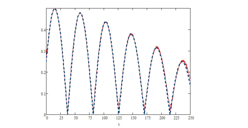
4.1 Evolution of|ρS12(t0)|(wheret0= gt/~) for the case that the system initially is
prepared in the|+ (t0)istate. Here we choseϕ=π/6 and ¯n= 50. The curve
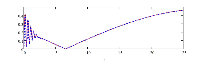
represented by dashed lines is plotted by using the approximate expression which we obtained from our pointer states, given by equation (4.96). The other curve with solid lines is obtained from the more exact expression of equation (4.82). . . 99 4.2 Short time evolution of|ρS12(t0)|for the case that the system initially is
pre-pared in the |bi state. Here we chose ϕ = π/6 and ¯n = 50. The curve represented by dashed lines is plotted by using the approximate expression which we obtained from our pointer states, given by equation (4.108). The other curve with solid lines is obtained from the more exact expression of equation (4.82). . . 102
Introduction
In this dissertation we study four different but closely related problems, within the context of quantum foundation and quantum optics. In essence, the corresponding four chapters, i.e. chapters 3 to chapter 6, build up the main part of my research contribution throughout the six years of my PhD career. The content of chapters 3 to chapter 6 of this dissertation has been prepared in paper format and in terms of four distinct papers for publication at Journal of Physics A and Annals of Physics. Wherever we refer to the papers within this dissertation, papers I [1] and II [2] respectively refer to the contents of chapters 3 and 6; while papersIII[3] and IV [4] respectively refer to the contents of chapters 4 and 5.
A part of the literature review and theoretical background is presented in chapter two. However, the main portion of the literature review and theoretical background for each of the four problems of this dissertation is presented at the beginning of the corresponding chapters; i.e. within chapters 3 to 6. Also each of the main chapters (chapters 2 to 6) has its own introduction section, where we introduce our motivation and the significance of the problem being studied within that chapter.
question mainly is composed of three distinct issues:
1. The problem of the preferred basis of measurement. What singles out the observable which will be measured through a specific system-apparatus interaction. For example, why a specific interaction with a two-level system would result in the measurement of the upper or lower levels of the system (the | ↑iand| ↓istates; i.e. the eigenstates of theσz operator) while another different interaction may result in the measurement of the eigenstates of say theσx operator. In other words, how can we know whether a specific interaction would result in realization of a specific basis of measurement or not? And how can we determine the observable which will be measured?
2. The problem of the nonobservability of interference effects. Why is it so difficult to observe quantum interference effects on macroscopic scales?
3. The problem of definite outcomes. Why do measurements have outcomes at all? And supposing that even we do know the observable which will be measured through a measurement interaction, what selects a particular outcome among the different pos-sible outcomes of measurement? This problem usually is referred to as the collapse problem. However, whether such a “collapse” of wave function is objective or subjec-tive still is a subject of debate.
Now we do know that from the abovementioned steps of measurement, the first two questions for sure can be described within the framework of the standard quantum me-chanics. However, as we will emphasize within chapters 2 and 6, decoherence cannot solve the collapse problem and it is mainly responsible in describing the second question, i.e. the problem of the nonobservability of interference effects. In fact, this dissertation is also mainly about the first two questions and the question of how to identify the generally time-dependent pointer states of the system and the environment (for a given total Hamiltonian describing a system-environment model), which are characterized as the states which keep their individuality and do not entangle with the states of another subsystem (rather than the collapse problem; which is the very last step of quantum measurement).
mechanics; (neither the Copenhagen interpretation nor the many-words interpretation of quantum mechanics). The Copenhagen interpretation assumes that the apparatus and the measuring devices are ruled by the laws of classical physics and not by the rules of quantum physics [5]; however, no longer this interpretation is taken that serious anymore, [6] and now the orthodox view of quantum mechanics tries to evade big assumptions like this. We also have not used the many words interpretation of quantum mechanics. In other words, what we have in this dissertation is not based on any specific interpretation; and the author believes that the followers of all interpretations would agree on the results of this dissertation; since they are merely based on the main structure of the standard quantum mechanics, and no further assumptions. In fact, we believe that before having a solution for the problem of definite outcomes using (or proposing) any interpretation for quantum physics is unjustifiable. Indeed, we have deliberately evaded talking much on the interpretations of quantum mechanics; since we especially wanted the reader’s attraction to be drawn more to the significance of this work with respect to the idea of entanglement, which is very important within the context of applied physics; rather than to make the reader think that this work is about interpretations of quantum physics and ideas which may not be that testable (like the many worlds interpretation and so on); or making him/her to think that this knowledge may not be important for applications. Therefore, here our main question is about entanglement and the states which may be immune to the entanglement with the environment; rather than how we should (or should not) interpret quantum physics. However, as we will see, the knowledge which we obtain through this quest for obtaining pointer states will also shed light on the questions which we have in the context of the problem of the preferred basis of measurement. We also will obtain some valuable knowledge about certain aspects of decoherence and decoherence of the models which we study in this research. Nonetheless, the problem of definite outcomes (the collapse problem) and whether it can be possible to describe this problem just within the framework of the standard quantum mechanics or not, still is a big question to be solved.
quantum control; which would suggest some ideas for future work. This dissertation is organized as follows:
After this introduction and in chapter 2 we review the concept of tracing over the environmental degrees of freedom and we discuss the main aspects of the phenomenon of decoherence.
In chapter 3 we discuss time-dependent pointer states and the problem of determina-tion of the preferred basis of measurement. We will also discuss the limitadetermina-tions in the current theories for determination of the preferred basis of measurement. As we will show, pointer states of a system in contact with an environment, which are characterized by their ability not to entangle with the states of another subsystem, quite easily may become time-dependent (for example due to the existence of non-commutative contributions in the Hamiltonian of the total composite system); and hence, generally one must distinguish be-tween pointer states of a subsystem, and the preferred basis of measurement, which consists of time-independent pointer states which can be realizedonly in certain regimes. We will present a general formulation for obtaining the generally time-dependent pointer states of the system and the environment and we will study the conditions under which the pointer states of the system may become time-independent; so that a preferred basis of measure-ment can be realized. The author believes that this chapter along with the fourth chapter are the most significant chapters of this dissertation, as well as his PhD research.
In chapter 4 we apply our formulation for obtaining time-dependent pointer states (dis-cussed in chapter 3) in order to obtain the time-dependent pointer states of the system and the environment for a spin-boson model which is generalized such that the Hamiltonians for the system ( ˆHS) and the interaction with the environment ( ˆHint) do not commute with each
decay in the evolution of coherences of the system).
In chapter 5 we do a similar calculation for the quantized atom-field model and in a nonresonance regime; i.e. we will obtain the time-dependent pointer states of the system and the environment for the quantized atom-field model and in a nonresonance regime. We will also obtain general expressions for the elements of the reduced density matrix of the system; and we will study the decoherence of the central system in our model.
In chapter 6 we will discuss some of the issues with Zurek’s proof of the Born Rule; and we will present our own proof of the Born rule.
[1] H. Daneshvar and G.W.F. Drake, “Time-dependent pointer states and determination of the preferred basis of measurement”, submitted toAnnals of Physics
[2] H. Daneshvar and G.W.F. Drake, “On Born’s rule, pk=|ψk|2, for quantum probabili-ties”, in preparation.
[3] H. Daneshvar and G.W.F. Drake, “Time-dependent pointer states of the generalized spin-boson model and consequences regarding the decoherence of the central system”, submitted toJournal of Physics A
[4] H. Daneshvar and G.W.F. Drake, “Time-dependent pointer states of the quantized atom-field model in a nonresonance regime and consequences regarding the decoherence of the central system”, submitted toJournal of Physics A
[5] M. Scholsshauer.Rev. Mod. Phys.76, (2004) 1267.
On tracing over the environmental
degrees of freedom and decoherence
2.1
Introduction
Tracing over the environmental degrees of freedom [1] is usually interpreted as averaging over the effect of the environmental degrees of freedom on the state of the system [2]. In the first part of this article, after exploring the exact meaning of tracing over the environmental degrees of freedom we will point out that the interpretation of tracing over the environment as “averaging” over the environment (as in [2]) in fact is not a good description for the process. Especially, it is not accurately true and it does not give us a clear insight about the process.
As we will discuss, the subtle difference between the meaning of the off-diagonal elements of areduced density matrix and the meaning of the off-diagonal elements of a density matrix before tracing over the environmental degrees of freedom is often neglected. This often produces ambiguity in interpretation and understanding of the phenomenon of decoherence. As an example, it is often falsely supposed that when the off-diagonal elements of the reduced density matrix are zero, the system under measurement is no longer in a pure state and we no longer have a superposition of possible states of the system. Indeed, the duty of the other important step of measurement, ie. the determination of definite outcomes (whose mechanism is yet to be understood), has often been attributed to decoherence; while it is important to know exactly what cannot be described by decoherence. We encounter this mistake in claims like the very common claim that “we do not observe a real Schrodinger cat, because ofdecoherence”. In this article we present a standard definition for the phenomenon of decoherence, as just one of the steps of the quantum-to-classical transition.
2.2
Tracing over the environmental degrees of freedom
There is a physical meaning behind tracing over the environmental degrees of freedom and in fact, it is not exactly averaging over the effect of the environment. As we will elaborately discuss in this section, tracing over the environmental degrees of freedom is in fact, the addition of different probabilities when there is a fine structure including the possible states of the system in addition to some degrees of freedom from another interacting system, when we are calculating the probabilities. 1 Also, tracing over the environmental degrees of freedom is the addition of different interference terms, when we are calculating the interference between different possible states of the system. Here, we will clarify the above statements using an example for tracing over the environmental degrees of freedom which is provided by the Jaynes-Cummings Model (JCM) of quantum optics [4].
Consider the state of the two-level atom (2LA) in the Jaynes-Cummings model, which involves a two-level atom with upper and lower levels that can respectively be represented
1
by|aiand|bi, interacting with a single-mode quantized electromagnetic field inside an ideal cavity, represented by creation and annihilation operators ˆa† and ˆa.
Suppose that ψan (ψbn) is the probability amplitude for finding the 2LA in the upper (lower) state and havingnphotons in the field. In the double basis set formed by{|a, ni}’s and {|b, ni}’s the global state of the system and the environment (the field) generally can be represented by the following matrix
|ψtot(t)i=
ψa0
ψa1
.. .
ψaN
ψb0
ψb1
.. . ψbN (2.1)
whereN is the maximum possible number of the field photons. Here note that although the state space for the state of the two-level atom (2LA) alone is a two dimensional space, the creation of correlations between the states of the 2LA and the field creates a fine structure which includes the states of the system in addition to possible states of the environment. The result can generally can be described in a 2N + 2 dimensional space.
Now, the diagonal element of the reduced density matrix of the system (the 2LA) is given by
ρ(red)11 =ha| X
n
hn|ψtotihψtot|ni |ai (2.2)
=X n
ha, n|ψtotihψtot|a, ni
=|ψa0|2+|ψa1|2+...+|ψaN|2.
system in the state |ai while having a certain number of photons in the field (we also note that the number states in the Hilbert space of the environment form a complete basis set). In this sense, tracing over the environmental degrees of freedom can be interpreted as the addition of different contributions that may make a possible state of the system happen.
In fact, the concept of reduced density matrices arises most naturally when we want to compute the expectation value of an observable ˆO in the Hilbert space of the system S, which is entangled with an environmentE (or more generally any other subsystem). Such an operator can be written as ˆO= ˆOS⊗IˆE, where ˆIE is the identity operator in the Hilbert space of the environment. Its expectation value generally can be computed using the trace rule,
hOiˆ =T r( ˆρOˆ), (2.3)
with ˆρ as the total density matrix for the global state of the system and the environment. As we will show here2, the trace operation of equation (2.3) can be simplified to a great
extent by analytically carrying out the tracing over the environmental degrees of freedom. Suppose that {|ψmi} and {|φni} are some orthonormal basis sets in the Hilbert spaces of the system and the environment respectively. Then
hOiˆ = Tr( ˆρOˆ) (2.4) =X
mn
hφn|hψm|ρˆ( ˆOS⊗IˆE)|ψmi|φni
=X m
hψm|(
X
n
hφn|ρˆ|φni) ˆOS |ψmi
=X m
hψm|(TrEρˆ) ˆOS |ψmi
=X m
hψm|ρˆSOˆS |ψmi = TrS( ˆρSOˆS),
where ˆρS is the reduced density matrix for the system. Thus, in order to obtain information about the result of measurements on the systemS, which is entangled with an environment
E, we can take advantage of the simpler mathematical object which is obtained by tracing over the environmental degrees of freedom.
2
The above discussion is in fact the source of the traditional interpretation of tracing over the environmental degrees of freedom as an “averaging” over the degrees of freedom of the environment. From the definition of the reduced density matrix, ˆρS = TrEρˆ=Pnhφn|ρˆ|φni, we can calculate its elements as
ρijS =X n
hψi|hφn|ρˆ|φni|ψji. (2.5)
Now, let us take a closer look to the above expression.
Let m0 and n0 be the the number of orthonormal basis states in {|ψmi} and {|φni} for the system and the environment respectively. The total state of the composite system generally can be represented by a column matrix of dimension N =m0n0, whose elements
in the double basis set formed by {|ψmi} and {|φni} are given by the scalar products
hψmφn|ψtoti. Also let hψmφn|ψtoti = ψmn. Now, we can calculate the elements of the reduced density matrix of the system as follows
ρijS =X n
hψi|hφn|ρˆ|φni|ψji (2.6)
=X n
hψi|hφn|ψtotihψtot|φni|ψji
=X n
ψinψjn∗ ,
where we have assumed that the global system starts in a pure state. For example, the diagonal elements read
ρiiS =
X
n
|ψin|2. (2.7)
(2.4)) be the eigenvectors of the system observable ˆOS with eigenvalues om
hOiˆ = Tr( ˆρOˆ) (2.8) =X
m
hψm|(
X
n
hφn|ρˆ|φni) ˆOS |ψmi
=X mn
om|ψmn|2.
Here, the meaning of “averaging” is embedded in summation over the complete set of eigenvalues corresponding to the system observable ˆOS, in addition to giving a weight to each eigenvalue by including the appropriate probabilities. However, note that generally we can not discriminate between averaging over the environment and averaging over the system since in general, the global state of the system and the environment is a highly entangled state. To clarify this point note that, only if the states of the system and the environment were not entangled, ie. if |ψtot(t)i = |ψS(t)i ⊗ |ψE(t)i (with |ψS(t)i and |ψE(t)i as some state vectors of the system and the environment respectively), we could rewrite equation (2.8) as
hOiˆ =X mn
om|hψm|ψSihφn|ψEi|2. (2.9)
By letting
hψm|ψSi=cm and hφn|ψEi=dn, (2.10)
this will read
hOiˆ =X mn
om|cm|2|dn|2. (2.11)
In this case also
TrE( ˆρ) =X n
hφn|ψtotihψtot|φni=
X
n
|dn|2|ψSihψS|. (2.12)
ie. if the states of the system and the environment are entangled, we can not write the global state of the total composite system in a product form like|ψtot(t)i=|ψS(t)i ⊗ |ψE(t)i and hence one cannot write the probabilities |ψmn|2 in equation (2.8) as the product of prob-abilities corresponding to the Hilbert space of the system and probprob-abilities corresponding to the Hilbert space of the environment, as in equation (2.11). As a result, one cannot discriminate between averaging over the environment and averaging over the system if the global state of the total composite system is an entangled one and the interpretation of tracing over the environmental degrees of freedom as “averaging” over the environment is by no means accurate.
Next, let us come back to the general expression in equation (2.6) in order to study the off-diagonal elements of the reduced density matrix which are given by
ρijS =X n
ψinψjn∗ ; with i6=j . (2.13)
For a two-state system like the two-level atom in our previous example of the Jaynes-Cummings model with upper and lower levels represented by |ai and |bi, this will read
ρ(Sab) =ψa0ψb∗0+ψa1ψ∗b1+...+ψaNψbN∗ . (2.14)
Note that if we denote the quantum state of the total composite system corresponding to the case that the two-level atom is in the upper or lower states respectively by|ψa(tot)i and
the state of the total composite system which can contribute in creating the interference (equation (2.14)).
2.3
Other notes on reduced density matrices and
decoher-ence
We note that, not all of the possible states of a composite system are necessarily able to interfere. A good example in the classical limit is two wavelets of light that meet each other at a specific point on a distant screen and having perpendicular polarizations, which of course will not interfere. They just add like different orthogonal components of a vec-tor without interfering; while both of them do exist at the same time and the (classical) superposition is still there. Similarly, when the off-diagonal elements of the reduced den-sity matrix are zero, it just means that we have no interference contribution to the total intensity (likeI =I1+I2+I12 with I12= 0). It does not necessarily mean that there is no
superposition of the states. In the quantum limit also, for example if we consider a pure state of the EPR type|ψi= √1
2(|+i1|−i2− |−i1|+i2, the reduced density matrix for any of
the two subsystems has no offdiagonal elements if the|±istates make an orthogonal basis. However, as we will describe, the fact that the reduced density matrix has no offdiagonal elements does not necessarily mean that there is no superposition of the two states of the systems. It just means that the two branches of the total system are orthogonal and hence, they are not able to interfere.
the composite system . Any states other than the pointer states of the system are subject to entanglement with the states of the environment; so that they lose their individuality (this means that the system cannot be ascribed with a well-defined state, due to the entanglement with the environment) and one cannot consider a one-to-one correspondence between some well-defined states from the system and some states from the environment [2, 5, 6].
Now once again let us consider a two-state system S with a preferred set of basis states|s0i and|s1i, which after premeasurement by the environment become coupled with
two states of the environment |ε0i and |ε1i respectively3. Before premeasurement by the
environment, which creates a one-to-one correspondence between the pointer states of the system and those of the environment, the global state of the system and the environment can be represented by
|ψSEi={α|s0i+β|s1i} ⊗ |εii, (2.15)
where |εii is the initial state of the environment before any coupling between the states of
the system and the environment. Also, after premeasurement is complete the global state of the system and the environment is given by
|ψSEi=α|s0i|ε0(t)i+β|s1i|ε1(t)i. (2.16)
The states appearing in the above equation are the pointer states of the system and the environment [2, 5, 6, 7]. Also, in writing the above equation it is assumed that the pointer states of the system are time-independent; so that they can represent the preferred basis of measurement. Now, the off-diagonal element of the reduced density matrix of the system is given by
ρS12=αβ∗.hε1(t)|ε0(t)i. (2.17)
while initially it simply wasρ(tot)12 =αβ∗. However, what really is a measure for the existence of superposition of the states is exactly the product αβ∗; for only when αβ∗ 6= 0, can we assume that the system is in the superposition of its two possible states. On the other hand, the off-diagonal element of the reduced density matrix includes another factor. i.e. the time-dependent overlap between the two pointer states of the environmenthε1(t)|ε0(t)i.
3
Hence, we may have αβ∗ 6= 0, while hε1(t)|ε0(t)i = 0 and thereforeρS12 = 0. In this case,
although both of the two basis states of the system|s0i and|s1istill can be measured in a
successive measurement on the state of the system, and in this sense the system is still in a superposition of its two possible states, the off-diagonal element of the density matrix is zero and this is because of the fact that after the states of the system are coupled to the corresponding states of the environment, as the overlap between the pointer states of the environment decreases from the initial value of hεi|εii= 1, the off-diagonal element of the
reduced density matrix of the system starts to vanish. This is exactly what happens during the phenomenon of decoherence by the environment.
In essence, this is the time evolution of the pointer states of the environment that causes the offdiagonal elements of the density matrix to vanish4. Here we should also mention that the study of several models of decoherence has revealed that the rate at which the overlap between the pointer states of the environment decreases (which also is a measure for the decoherence rate) often is increased as we increase the number of the environmental degrees of freedom [6, 7, 8, 9].
Hence, it is important to distinguish between the meaning of the off-diagonal elements of a density matrixbefore andafter tracing over the environmental degrees of freedom. As we discussed, although the off-diagonal elements of a density matrix before tracing over the environmental degrees of freedom exactly refer to the existence of superpositions, we should note that after tracing over the environmental degrees of freedom, they just refer to interference. Furthermore, we should exactly clarify what we mean by “coherence” in the word “decoherence”. Indeed, if by “coherence” we refer to the existence of superposition of pointer states, then “decoherence” of course cannot be a good description for the suppression of the off-diagonal elements of density matrices; since as we discussed, up to this stage of a quantum measurement we can only conclude that such “coherence” between different components of the pure state of a quantum system can only be delocalized into the larger
4
composite system as a result of quantum entanglement, and it is not yet disappeared (see eqs. (15), (16) and (17)). However, we can justify the use of the word “decoherence” if by “coherence” we refer to the phase coherence among different interference terms in the summation represented in equation (2.13), in which when there is phase coherence between different contributions, they will add constructively and we expect to have interference.
The above point actually is in contrast with what is often advocated by many authors regarding decoherence. In fact, the word “coherence” is often wrongly used by taking it to be synonymous with superposition. For example, in his paper entitled “the decoherence puzzle” [10], Stamp interchangeably uses the two words of “coherence” and “superposition” instead of each other; eg. when he uses the expression “coherence (i.e., superpositions)”. Many other authors use this word as equivalent to superposition. However, it is important to correctly use this word by attributing it to the phase coherence rather than superpositions; since its usage as equivalent to quantum superposition can imply that decoherence is related to the loss of superpositions. As another example, Vedral in his book entitled Introduction to quantum information science [11] writes:
Dissipation implies loss of energy to the environment, while decoherence im-plies the loss of coherence, ie. superpositions, and may not involve any energy exchange.
We should also note that reduced density matrices generally do not specify the state of the system; in the sense that by looking at a density matrix we cannot discern if the system, which it intends to describe, is in a pure or in a mixed state. This can also be understood by noting that the reduced density matrix corresponding to the pure state of a composite system with environmental pointer states that are orthogonal literally has no difference with a density matrix that can also represent a mixed state. For example, for a pure state of the EPR type
|ψi= √1
density matrix reads
ˆ
ρ (1)= 1
2{|+i1h+|1+|−i1h−|1}. (2.19) Here we emphasize that in the state of the total composite system, represented by equation (2.18), we do have a superposition of the states of each subsystem; as we have coexistence of the |+i1(2) and |−i1(2) states of each subsystem;although each of the|+i1(2)and |−i1(2)
states is correlated with some corresponding states from the other subsystem, and we cannot ascribe a state vector to each of the subsystems alone5.
Now, note that if we consider the density matrix corresponding to a mixed state of the total composite system given by
ρtot= 1
2{|+i1h+|1|−i2h−|2+|+i2h+|2|−i1h−|1}, (2.20) tracing over the degrees of freedom of the second subsystem obviously would result in a reduced density matrix for the first system as that of equation (2.19), which was the reduced density matrix which we obtained from the total density matrix of thepure state, given by equation (2.18).
Now if we consider the purity, Tr(ρ2), for the reduced density matrix given by equation (2.19), it would be equal to 12; which based on that one might conclude that the system is in a mixed state. However, we do know that the reduced density matrix of equation (2.19) could equally be obtained from the pure state of equation (2.18),or the mixed state represented by the total density matrix of equation (2.20). Therefore, although our reduced density matrix will show the same observable properties no matter if it is obtained from the pure state of equation (2.18) or the mixed state of equation (2.20), by having such a reduced density matrix we cannot conclude whether we have the superposition of the states of the system, or the system is part of a composite system in a mixed state6.
5It is true that here we cannot ascribe a well-defined state to the system alone. But,none of the possible branches of the system yet are selected at this stage of a measurement. So, they still coexist at this step; although they coexist while they are coupled with some corresponding pointer states from the environment, through a perfect one-to-one correspondence between the pointer states of the system and the environment.
6The essence of this argument has been established in another way through the so-called purification
As another explanation, by looking at equation (2.17) we see that if we have time-independent pointer states for the environment (i.e. system 2 in this example) which are orthogonal to each other, definitely the coherences of the reduced density matrix of the system (i.e. system 1 in this example) will be zero. However, as we discussed, this necessarily does not mean that we do not have the superposition of the states of the system. Regarding the reduced density matrix of equation (2.19) also, the fact that it does not have any offdiagonal elements simply is a result of having h+|−i2 as equal to zero (see equations
(2.17) and (2.18)); and necessarily it does not mean that we do not have a superposition of the|±i1 states.
In essence, one should be careful that the so called “purity”, defined by Tr(ρ2), is not a
measure for the purity of the state of the system when we are considering reduced density matrices. Moreover, decoherence is not responsible for conversion of superpositions into mixed states, as it only makes the pointer states of the environment orthogonal to each other; removing the possibility of any interference effects (see equation (2.17)). This point also is in contrast to claims which one often encounters, like the following claim by Zurek [13]
... For our purposes, the effect of the last term on quantum superpositions is of greatest interest. I shall show that it destroys quantum coherence, elimi-nating offdiagonal terms responsible for quantum correlations between spatially separated pieces of the wave packet. It is therefore responsible for the classical structure of the phase space, as it converts superpositions into mixtures of local-ized wave packets which, in the classical limit, turn into the familiar points in phase space.
We finish this article by discussing the relationship between the unitarity of the evolution of the total system, which is imposed by evolution according to the Schr¨odinger equation, and the decoherence of the state of the system.
expect that the evolution of the global state of the system and the environment preserves the norm of the total composite system. Also, as each of the subsystems that make the total composite system cannot be regarded as a closed system, naturally we do not expect that the evolution of each of the subsystems follows a unitary procedure. Nonetheless, in what follows we carefully examine the unitarity of the evolution of the global state of the system and the environment and its consequences, with specific attention to the case that the pointer states of the system necessarily are not orthogonal. This can be useful with respect to certain experimental settings for the study of the interference effects in which the pointer states of the system necessarily are not orthogonal.
Again let us consider the global state of the system and the environment represented by equation (2.16), which is created after the interaction between the two-level system S
(initially prepared in the state |ψSi = α|s0i+β|s1i) and the environment E determines
are time-dependent, let us rewrite equation (2.16) as follows
|ψSEi=α|s0(t)i|ε0(t)i+β|s1(t)i|ε1(t)i. (2.21)
We emphasize that the states appearing in the above equation must be discriminated from the instantaneous Schmidt states which can be obtained by diagonalizing the density matrix at each instant of time and which generally are not unique. Mainly because of the fact that the pointer states of the system and the environment, appearing in the diagonal state of the total composite system in the above equation, are the states which are characterized by their ability not to entangle with the states of another subsystem,7 and one can examine this property of candidate pointer states at least in principle by solving the Schr¨odinger equation8. However, Schmidt states generally are not unique, and in addition to that they necessarily do not exhibit the quasiclassical properties of pointer states and hence, generally are not expected to preserve a one-to-one (system-environment) correspondence amongst themselves when evolved according to the Schr¨odinger equation. Moreover, the states appearing in equation (2.21) are not necessarily orthogonal at all times; while by definition the Schmidt states must be orthogonal within themselves at all times.
Coming back to our discussion regarding the unitarity in the evolution of the state of the total system, now the norm of the state of the total composite system is related to
hψtot|ψtoti=|α|2 hs0(t)|s0(t)i hε0(t)|ε0(t)i (2.22)
+|β|2 hs1(t)|s1(t)i hε1(t)|ε1(t)i
+αβ∗ hs1(t)|s0(t)i hε1(t)|ε0(t)i+ c.c.
As we discussed, decoherence is related to the suppression of the factor hε1(t)|ε0(t)i of the
third term in the above equation. Nowif the pointer states of the system are orthogonal, 7
This is often referred to as thestability criterion for determination of pointer states.
8In other words, pointer states of a system emerge dynamically, as a result of the natural evolution of the
we note that the third term in equation (2.22) will be zero; no matter how big is the factor
hε1(t)|ε0(t)i and hence, no matter if decoherence occurs or not. However, nonorthogonal
pointer states are not a priori forbidden; as they can arise in certain experimental settings where we can observe interference effects. As an example, the pointer states of the system in the JCM (as are discussed in appendix A) are not orthogonal at all times. Or as another example in the context of quantum optics, it has been shown that for a harmonic oscillator interacting with an environment in thermal equilibrium and in the weak coupling limit the interaction between the system and the environment will result in the superselection of coherent states [4, 15] as the pointer states of the system which are characterized by max-imal stability [15]; while the coherent states are well known to be nonorthogonal amongst themselves.
In such cases like that of the Jaynes-Cummings model where the pointer states of the system are not orthogonal at all times, although none of the two factorshs1(t)|s0(t)i and
hε1(t)|ε0(t)iof equation (2.22) is uniformly equal to zero, still we expect the last two terms
in equation (2.22) to be zero; since hψtot|ψtoti, given by equation (2.22), must always (i.e.
for all possible α and β) be equal to the unity; including for the case thatα = 0 orβ = 0. Therefore, we must have hs0(t)|s0(t)i × hε0(t)|ε0(t)i=hs1(t)|s1(t)i × hε1(t)|ε1(t)i= 1 and
hs1(t)|s0(t)i×hε1(t)|ε0(t)i= 0. Only in this case the norm of the state of the total composite
system will always be preserved, although decoherence is in progress all throughout the evolution of the state of the total system due to the decay of the overlap between the pointer states of the environment hε1(t)|ε0(t)i.
The last of the above conditions is possible only if at those probable times for which
hε1(t)|ε0(t)i 6= 0 we have the zeros ofhs1(t)|s0(t)ito take place; and wheneverhs1(t)|s0(t)i 6=
0 we have the zeros of hε1(t)|ε0(t)i 6= 0 to take place. In appendix A considering the
approximation for obtaining the pointer states of the Jaynes-Cummings model, given by
t~√n/¯ g (with ¯nas the average number of photons in the environment) [8], we show how this condition exactly is satisfied for t ~
√
¯
system in a diagonal form in terms of pointer states); although for the Jaynes-Cummings model one may not be able to do the same kind of calculation in any analytical way for arbitrary large times.
In essence, although decoherence progresses and the overlap between the pointer states of the environment constantly decreases with time, the last two contributions in the norm of the state of the total composite system (equation (2.22)) are always zero, and this way it is guaranteed that the norm of the state of the total composite system is preserved. The generalization of the above discussions to the case that the system has more than two possible states can be an interesting problem to be explored.
2.4
Conclusion
We studied the exact meaning of tracing over the environmental degrees of freedom as a procedure that (by considering the fine structure which is created due to the formation of correlations between the states of the system and those of the environment) calculates the probabilities for finding the system in specific states, by adding all “fine-probabilities” for finding the system in specific states, when we are calculating the diagonal elements of the reduced density matrix. It also merely calculates the interference between two possible states of the system, by adding the contributions from the interference of corresponding branches of the global state of the system and the environment, when we are calculating the off-diagonal elements of the reduced density matrix (equation (2.13)).
conversion of superpositions into mixed states as it only makes the pointer states orthogonal to each other; removing the possibility of any interference effects. Also the so-called purity of a reduced density matrix is not actually a measure for the purity of the state of the system.
We note that the presented discussions are not necessarily in favor of an Everettian interpretation of quantum mechanics; if we keep in mind that decoherence is just one of the steps in the procedure of the quantum-to-classical transition, which only refers to the interference effects. Hence, although decoherence provides us with a description for the usual nonobservability of quantum interference effects in macroscopic scales, but the mechanism by which we observe definite outcomes of measurement still remains a fundamental question to be answered.
[1] L. Landau. Z. Phys.45, (1927) 430.
[2] M. Schlosshauer.Decoherence and the Quantum-to-Classical Transition, Berlin Heidel-berg: Springer (2007).
[3] M. Born. Z. Phys.37, (1926) 863;
J.A. Wheeler and W.H. Zurek (Eds.). Quantum Theory and Measurement, Princeton: Princeton University Press, (1983) 52-55.
[4] M.O. Scully and M.S. Zubairy. Quantum Optics, Cambridge: Cambridge University Press (1997).
[5] W.H. Zurek. Phys. Rev.D24, (1981) 1516.
[6] W.H. Zurek. Phys. Rev.D26, (1982) 1862.
[7] W.H. Zurek. Rev. Mod. Phys.75, (2003) 715.
[8] J. Gea-Banacloche.Phys. Rev. A 46, (1992) 7307.
[9] M. Schlosshauer.Decoherence and the Quantum-to-Classical Transition, Berlin Heidel-berg: Springer, (2007) 137-138. In the discussion on the decoherence due to scattering of air molecules it is shown that the decoherence time is inversely proportional to the scattering constant; while the scattering constant is proportional to the number density of particles in the environment.
[10] Stamp.Studies in History and Philosophy of Modern Physics 37, (2006) 467-497.
[11] Vedral.Introduction to quantum information science, Oxford: Oxford University Press, (2006) 160.
[12] M.A. Nielsen and I.L. Chuang. Quantum Computation and Qunatum Information, Cambridge: Cambridge University Press (2000).
[14] J. Gea-Banacloche.Phys. Rev. A 44, (1991) 5913.
Time-dependent pointer states and
determination of the preferred basis of
measurement
3.1
Introduction
This chapter is organized as follows:
In section 3.2 (which is our introductory review and discussion section to better identify what the problem is) after reviewing the orthodox theory for determination of the pointer states of measurement we discuss an important restriction of this theory regarding the so-calledcommutativity criterion for determination of the pointer states. In fact, we will show that the pointer states of the system and the environment, which appear in the diagonal state of the total composite system
|ψSEi= N
X
k=1
αk|ski|εki (3.1)
tativity criterion, first introduced by Zurek [1-3], although sufficient in order to assure the requirement of having a faithful measurement, is too restrictive and generally does not hold valid for the pointer states of measurement in all situations. In other words, it is not the minimal condition for having a faithful measurement. We will show that the commutativity criterion can be validonly in certain regimes and under the specific conditions in which the pointer states of the system2 are independent of time.
In section 2 we will also very briefly review some of the other predictability criteria which have been exploited to obtain the pointer states of measurement. We will discuss some of the restrictions and difficulties which one should expect while using these methods. In section 3 we present a method in order to calculate the (generally) time-dependent pointer states of the system and the environment for an arbitrary total Hamiltonian defining the system-environment model and in section 4, using this method, we will exactly discuss under which conditions we can have time-independent pointer states; and also how we can predict the preferred basis of measurement in each of the corresponding regimes. As we will see, only under specific conditions time-independent pointer states can be realized; therefore a preferred basis of measurement does not necessarily exist in an arbitrary regime.
In section 5 we will discuss the significance of our theory more elaborately and will conclude.
outside our system of interest and hence it can include the apparatus as well.
2
3.2
Review and discussion: identifying the problem
3.2.1 The Schmidt decomposition
Before proceeding to the question of the pointer states of measurement we would talk about the oldSchmidt Decomposition Theorem [4] which states that an arbitrary pure state|Ψi
of the composite system AB, made up of two subsystems A and B endowed with Hilbert spacesHA and HB, can always be written in a diagonal form
|Ψi=X i
λi |aii |bii, (3.2)
where the Schmidt states |aii and |bii are orthonormal amongst themselves and form the so-called Schmidt bases of HA and HB respectively, and the expansion coefficients λi gen-erally are some complex numbers fulfilling P
i|λi|2 = 1. Moreover, it is shown that this decomposition is unique if and only if the expansion coefficientsλiare all different from one another. Note that the above statement basically refers to the fact that in describing the total state of a composite system in a diagonal form with orthonormal basis states generally there is abasis ambiguity, as the diagonal decomposition is not always unique.
We also note that the reduced density matrices ˆρA and ˆρB for the two subsystems which are obtained by tracing operation will be diagonal in the Schmidt bases {|aii} and
{|bii}, as one can easily verify, because of the fact that these states are orthogonal amongst themselves. Therefore, the Schmidt bases correspond to the orthonormal basis states which diagonalize the reduced density matrices.
3.2.2 Premeasurement by the environment
Von Neumann scheme [5] for quantum measurement which states that if the system starts out in a superposition of the basis states |sii,
|ψi=X i
ci|sii (3.3)
then, the system-apparatus combination will evolve according to
|ψi|ari= (
X
i
ci|sii)|ari → |ψi=
X
i
ci|sii|aii (3.4)
where |ari is the initial “ready” state of the apparatus. We note that the Von Neumann scheme described by equation (3.4), which usually is also referred to as premeasurement, can be obtained just by assuming the requirement of the faithful measurement of the state of the system initially prepared in the state|sii, i.e. the requirement that|sii|ari → |sii|aii and the linearity of Schr¨odinger’s equation.
3.2.3 Example: evolution of the two-level atom in the Jaynes-Cummings model
To clarify this better here we present a physical example, represented by the evolution of the two-level atom in the Jaynes-Cummings model (JCM) of quantum optics, in order to show how in practice a diagonal state withtime-dependent pointer states can be created as a result of the natural evolution of the global state of the system and the environment.
Consider the state of the two-level atom in the Jaynes-Cummings model of quantum optics which involves a two-level atom, with upper and lower levels that can respectively be represented by |ai and |bi, interacting with a single-mode quantized electromagnetic field inside an ideal cavity, represented by creation and annihilation operators ˆa† and ˆa. For exact resonance and in the rotating-wave approximation, the interaction Hamiltonian for the composite system can be written as
ˆ
Hint=~g(ˆa†σ−+σ+ˆa). (3.5)
where g = −%12.ˆ
q w
2~ε◦V is the atom-field coupling constant, with %12 = eha|r|bi as the atomic electric-dipole transition matrix element. (ˆis the field polarization vector,ω is the atomic transition frequency which is taken to be resonant with the frequency of the cavity eigenmode, and V is the cavity mode volume). Also σ+ and σ− are the atomic flipping operators given by
σ+=|aihb| and σ−=|biha|. (3.6)
Consider the field to be initially in the coherent state|νi
|Φfield(t0)i=|νi=
∞
X
n=0
cn|ni; with cn= e−12|ν|
2
νn
√
n! , (3.7)
where|ν|2 = ¯n is the average number of photons in the coherent state, andν =|ν|e−iφ. In general, the exact solution for an initial atomic state |ψatom(t0)i =α|ai+β|bi and a field
state initially prepared in the coherent state, is a highly entangled state of the field and the atom [6]. However, Gea-Banacloche [7] has shown that for a large average number of photons, if we consider the evolution of the initial atomic states |+i and |−i, defined by
|±i= √1
2(e
(here φ is the same as the phase of ν = |ν|e−iφ), the evolution of the global state of the system and the field (the environment) would be very interesting. Gea-Banacloche proved that when the initial atom-field state is |±i|νi, in the limit of ¯n→ ∞ the global state of the two-level atom (2LA) and the field will evolve as follows:
|±i|νi|t=0→ √1
2(e
−iφe∓igt/(2√n¯)|ai ± |bi)× |Φ±(t)i, (3.9)
where
|Φ±(t)i= e−¯n/2 ∞
X
n=0
¯
nn/2
√
n!e
−inφe∓igt√n|ni, (3.10)
gives us the time evolution of the state of the field. This result holds for any time, provided that t goes to infinity slowly enough to have t/n¯ → 0. Since the time scale for the JCM revivals is tR = 2π
√
¯
n/g [6], tR/¯n → 0 as ¯n → ∞ (a typical value for g/2π is 44 kHz in
a micromaser experiment [7]). Hence, the approximate solution in equation (3.10) holds accurately over a large number of revivals, as long as ¯nis large enough.
The states |+i and |−i form a basis set for the two-level atom (2LA); therefore, the evolution of any other initial atomic state with an initial coherent field can be expressed as a linear combination of the evolution of |+i|νi and |−i|νi.
(γ|+i+δ|−i) |νi|t=0→γ |+ (t)i |Φ+(t)i+δ | −(t)i |Φ−(t)i
with |+ (t)i= e
−iφe−igt/(2√¯n)|ai+|bi
√
2 (3.11)
and | −(t)i= e
−iφe+igt/(2√n¯)|ai − |bi
√
2 .
The time-dependent states| ±(t)iand|Φ±(t)iappearing in the above equations arethe pointer states of the system (the 2LA) and the environment (the field) which are charac-terized by their ability not to entangle with each other. As we observe, in the limit of large ¯
¯
n, when the 2LA is initially prepared in one of the two states |±i, the field and the atom never entangle; while equations (3.9) and (3.11) indicate that for any initial atomic state other than the |±i states, the states of the field and the atom will not remain separated and they entangle throughout the interaction. Also, equation (3.11) indicates that for an arbitrary initial atomic state and in the limit of large ¯n, there is always a one-to-one corre-spondence between a (preferred) set of pointer states from the system (the 2LA) and some corresponding states of a field which is initially prepared in a coherent state.
In essence, we observe that in the limit of large ¯n and for an initial coherent field, in fact the coherent field does a Von Neumann premeasurement on the state of the 2LA; which makes the global state in a diagonal form and superselects a preferred set of pointer states of the system. However, here the premeasurement by the field definitely is not an ideal premeasurement, as the initial atomic states |±i evolve by acquiring a phase factor e∓igt/(2
√
¯
n); except fortt
R, for which this change is negligible and the right hand side of
equation (3.11) can be approximated by γ |+i|Φ+(t)i+δ |−i|Φ−(t)i.
3.2.4 Schmidt states versus pointer states
It can be shown that in the limit of ¯n → ∞, which corresponds to the classical limit for which equations (3.9) to (3.11) are valid, the field states |Φ+(t)i and |Φ−(t)i almost
promptly become orthogonal [7]. However, as is obvious from equation (3.11), the pointer states of the system are not orthogonal at all times; and hence the diagonal state of the total composite system (represented by equation (3.11)), which is created after premeasurement, cannot represent a Schmidt decomposition at all times; as by definition the Schmidt states of the system and the environment must be orthogonal amongst themselves.
The Schmidt states obtained by diagonalizing the density matrix of the system at each instant of time necessarily are not the same as the pointer states at corresponding times; even in certain regimes and those times long enough so that the pointer states of the sys-tem and the environment can be considered as orthogonal amongst themselves. (For our example of the JCM the pointer states of the system are almost orthogonal provided thatt
the pointer states of the environment, given by equation (3.10), become orthogonal within a time of the order of 1/g due to decoherence, as was proved by Gea-Banacloche [7]). This is basically because of the fact that the Schmidt basis obtained this way will not necessar-ily exhibit the quasiclassical properties which are characteristic of the dynamical pointer states of measurement. In fact, as we described, the pointer states of the system emerge dynamically as those states that do not entangle with the environment; while the Schmidt states (which generally are not unique) necessarily are not robust against the entanglement with the environment. Hence, the pointer states of measurement generally cannot be ob-tained simply by diagonalizing the instantaneous density matrix of the system. (However, it is shown that only when the Schmidt states of the system are very nearly degenerate they can be significantly different from those environment-selected pointer states which are orthogonal amongst themselves (i.e. pointer states at certain regimes and sufficiently long times, so that they can be considered as orthogonal); while they are almost the same as the environment-selected pointer states whenever they are far from degeneracy and the pointer states of the system and the environment can be considered as orthogonal amongst them-selves. The interested reader for example can refer to the interesting article by Albrecht [8]. This result in fact is just as we expect from the condition for the uniqueness of the Schmidt decomposition; since when the Schmidt states of the system are very nearly de-generate, this indicates that not all of the expansion coefficients in the diagonal state of the total composite system (equation (3.2)) are different and hence the Schmidt states are not unique. Therefore, in this case the Schmidt states which we obtain by some procedure necessarily will not be the same as the instantaneous pointer states of measurement which likewise diagonalize the state of the total composite system, but in addition to that do not entangle with the states of another subsystem at a subsequent time).
3.2.5 The commutativity criterion
correspon-dence between the states of two subsystems, no longer can we have a faithful measurement. For example if at an initial time t0 the states of the system which appear in the diagonal
state of the total composite system are the two states|ψ1(t0)i and |ψ2(t0)i, then they can
be considered as the instantaneous pointer states of the system if their further interaction with the environment preserves the one-to-one correspondence with the environment. In other words their evolution must be of the following form
|ψ1(t0)i|E0i → |ψ1(t)i|E1(t)i and |ψ2(t0)i|E0i → |ψ2(t)i|E2(t)i. (3.12)
Now if we consider a superposition of these states at an initial timet0 like
|ψ±(t0)i=α |ψ1(t0)i ±β |ψ2(t0)i, with αβ6= 0 (3.13)
then, due to the interaction with the environment such a state will evolve according to
|ψ±(t0)i|E0i →α |ψ1(t)i|E1(t)i ±β |ψ2(t)i|E2(t)i. (3.14)
This means that any superposition of|ψ1(t0)iand |ψ2(t0)i states (the states which appear
in the diagonal state of the total composite system and do not entangle with the states of the environment) immediately entangles with the environment and hence it will lose its individuality and become unobservable. Indeed, the pointer states of the system emerge dynamically as those states that are the least sensitive, or the most robust, to the interaction with the environment; in the sense that they do not entangle with the environment. This is commonly referred to as the stability criterion for the selection of the pointer states [1, 2, 3]. In essence, some states are robust in spite of the environmental interaction, while other states rapidly entangle with the environment, lose their individuality and therefore become unobservable in practice. However, the information about only those states of the system that do not entangle with the environment can be passed all the way to the observer and these are the pointer states of measurement.
measurement. In section 3 we discuss why indeed the states which may be able to satisfy the requirement of faithful measurement generally are expected to be time-dependent. Also, in section 4 we will discuss the exact conditions under which the pointer states of measurement can be time-independent, so that a preferred set of basis states can exist as the basis of measurement.
With this introduction, now our ultimate goal is to find the preferred basis of measure-ment. However, we must first identify the pointer states of the system for an arbitrary total Hamiltonian defining the system-environment model. As we described, our general selection criterion is given by thestability criterion; i.e. the set of the pointer states of the system is given by those states of the system that do not entangle with the environment. In other words, they keep their individuality; so that they are able to hold a one-to-one corre-spondence with the states of the environment. In order to find these states, we should look for system states|si(t)i(like those of equation (3.11) for the JCM) such that the composite system-environment state, when starting from a product state|si(t0)i|E0iatt= 0, remains
in the product form |si(t)i|Ei(t)i at all subsequent times t > 0 under the action of the total Hamiltonian. Now we show that the commutativity criterion for the determination of the pointer states of measurement, first introduced by Zurek [2, 3], although is sufficient in order to assure the requirement of having a faithful measurement, it is too restrictive and generally does not hold in all situations. In other words, it is not the minimal condition for having a faithful measurement.
Two regimes are often considered. In the quantum measurement limit the interaction between the system and the environment is so strong as to dominate the evolution of the system. Therefore, in this limit it is assumed that the intrinsic dynamics of the system and the environment is negligible in comparison with the evolution induced by the interaction. i.e.
ˆ
H≈Hˆ0; (3.15)
and hence, the evolution of the composite system-environment state is approximately given by the evolution operator e−iR0tHˆ0(t
0)dt0 .
Hamiltonian for the system almost dominates the interaction between the system and the environment as well as the self-Hamiltonian of the environment. Hence, in this limit which frequently is called as the quantum limit of decoherence, the following approximation is assumed
ˆ
H≈HˆS. (3.16)
As we show in section 4, the result of these approximations is that the pointer states of the system turn out to be independent of time (unlike those of the JCM in equation (3.11) which are obtained for the “exact-resonance” regime).
In his famous 1981 paper Zurek argued that in the quantum measurement limit the preferred set of pointer states for the system should be given by those states of the system that are eigenstates of the part of the interaction Hamiltonian ˆH0 pertaining to the Hilbert space of the system; since in this case we have
e−iR0tHˆ0(t 0)dt0
|sii|E0i=|sii e−i Rt
0(λi(t 0) ˆE)dt0
|E0i ≡ |sii|Ei(t)i, (3.17)
provided ˆH0 = ˆS⊗Eˆ; with ˆS and ˆE denoting some operators in the Hilbert space of the system and the environment respectively; and ˆS |sii = λi|sii. As we see from equation (3.17), in this case the state of the system does not entangle with the state of the envi-ronment. (If we consider the more general form of the interaction Hamiltonian given by
ˆ
H0 =P
αSˆα⊗Eˆα, then a sufficient condition for{|sii}to form a set of pointer states of the system is that the|siibe simultaneous eigenstates of all the system operators ˆSα.)
Equivalently, if we define the pointer observable as the observable for the system whose eigenstates are these pointer states|sii of the system, i.e.
ˆ
OS =
X
i
oi|siihsi|, (3.18)
since the|siiare eigenstates of ˆH0, it follows that ˆOS must commute with ˆH0,
[ ˆOS,Hˆ0] = 0. (3.19)
identifying the pointer states of a system (i.e. as we will discuss here, in many situations the pointer states of the system, which are characterized by their ability not to entangle with the environment, are time-dependent and do not satisfy the commutativity criterion); since we note that if the pointer states of the system are eigenstates of the Hamiltonian, as Zurek has proposed, for an interaction Hamiltonian which does not explicitly depend on time (like that of our example of the JCM at the zero-detuning regime) the most that can change about the pointer states of the system under the effect of the evolution operator is an overall phase factor and basically they would remain unaltered under the effect of the evolution operator. In other words, Zurek’s pointer states are basically independent of time. However, the point is that in order to satisfy the requirement of faithful measurement the pointer states of the system do not have to be independent of time like Zurek’s pointers. For example a one-to-one correspondence between some well-defined states of the system and some states from the environment is preserved in our example represented by the JCM (equation (3.11)); while as we saw, the pointer states which appear in the diagonal state of the total composite system in this example clearly depend on time.
3.2.6 Bloch vector and determination of the preferred basis of measure-ment
The reduced density matrix of a two-level system ˆρS(t) generally can be expressed in terms of the Bloch vectorR(t)≡(Rx, Ry, Rz) [9] as follows
ˆ
ρS(t) = 1
2( ˆI+R(t).σˆ) = 1
2( ˆI+Rxσx+Ryσy+Rzσz); (3.20) from which one can easily verify that the Bloch vector components must be defined by
Rx =ρab+ρba Ry =i(ρab−ρba) and Rz =ρaa−ρbb. (3.21)
In the above equation we used the notationρab=ha|ρˆS(t)|bi (with|aiand |bi representing a complete set of basis states for the two-level system) and etc.
The Bloch vector here can be interpreted as the polarization of the state of the two-level system. This is because the direction ofR tells us into what set of eigenstates the reduced density matrix of the system can be decomposed. For example, ifRx =Ry = 0 andRz 6= 0 then
ˆ
ρS(t) = 1
2( ˆI+Rzσz) = 1 2
1 +Rz 0 0 1−Rz
; (3.22)
therefore, ˆρS will commute with σz and can be decomposed in terms of the eigenstates of
σz. As a result, generally speaking in a certain regime of the parameter space only if the components of the Bloch vector settle in some asymptotic values att→ ∞, can we conclude that at sufficiently long times there can exist a preferred basis of measurement represented by the eigenstates of ˆρS. Otherwise, i.e. if the Bloch vector constantly changes its direction, a preferred basis of measurement cannot be realized in the corresponding regime.