Frequent Pattern Mining Using Hyper Path in
Hypergraphs
Dr. Sabeen S
Associate Professor, Department of Computer Applications, Jaya Engineering College, Chennai, Tamilnadu, India
ABSTRACT: Hypergraph is used as a tool to model and solve some classes of problems arising in frequent pattern mining. Hypergraph is a generalization of a graph wherein edges can connect more than two vertices and are called hyperedges. Efficient algorithms for generating the hypergraph model and extracting frequent patterns for association
rule mining are proposed in this paper. An algorithm is introduced which generates the Hypergraph model D and which
also simultaneously computes several other measures such as frequent items, nonfrequent items, total number of hyperedges, length of a largest transaction, frequency of occurrence of various nodes and the number of occurrences of
each hyperedge in D. The second algorithm generates all the patterns of the transaction database using the above data
structure. This algorithm can be modified to extract frequent patterns. The third algorithm deals with extraction of
frequent subhypergraphs induced by all frequent patterns L. The study shows that this new approach has high
performance in various kinds of data, which outperforms the previously developed algorithms in different settings, and is highly scalable in mining different databases.
KEYWORDS: frequent pattern, hypergraph, hyperedge, hyperpath, association rule, path system, transaction database,
I. INTRODUCTION
A hypergraph introduced by Berge C [1] is a set V of vertices and a set of non-empty subsets of V, called hyper
edges. Unlike graphs, hypergraphs can capture higher-order interactions in social and communication networks that go beyond a simple union of pair wise relationship. Just as graphs naturally represent many kinds of information in mathematical and computer science problems, hypergraphs also arise naturally in important practical problems, including circuit layout, numerical linear algebra, etc. A hypergraph is a natural extension of a graph obtained by
removing the constraint on the cardinality of an edge: any non-empty subset of V can be an element (a hyper edge) of
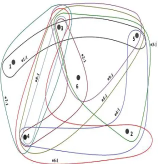
the edge set E( see Figure 1). For example, let X = { x1, x2 ,x3 ,x4 ,x5, x6, x7 ,x8} and E = { E1, E2, E3, E4, E5, E6 } = {{ x3 ,x4 ,x5}, {x5,,x8},{ x6, x7 ,x8},{ x2 ,x3, x7 },{ x1, x2 },{ x7}}. This hypergraph is given in Figure 1.
Figure 1 Hypergraph
tends to concern questions similar to those of graph theory, such as connectivity and colorability, while the theory of set systems tends to ask non-graph-theoretical questions.
II RELATED WORK
The problem of mining frequent itemsets arose first as a sub problem of mining association rules Agrawal et al (1993). The frequent itemset mining problem has been formulated as the computational relevant step in association rule mining. Frequent itemset mining problem appears as a sub problem in many other data mining fields like association rule discovery[10], correlations, classification [11] clustering [12], web mining [13] and [14]. The original motivation for searching association rules came from the need to analyse the supermarket transaction data, that is, to examine customer behavior in terms of the purchased products. Association rules describe how often items are purchased together. For a given sequence of itemsets, we have to find itemsets that are contained as a subset in more than a given number of elements of the sequence.
III. HYPERGRAPH AND HYPERPATH
Let V be a finite set and E a family of subsets of V. If then the couple D = (V, E) is
called a hypergraph. Each element is called a vertex and each element a hyperedge. A hyperpath
between two vertices u and v is a sequence of hyperedges such that , and for
i=1,2,….,m− 1. A hyperpath is simple if non-adjacent hyperedges in the path are non overlapping, that is,
, , i ±1. Obviously any transaction database is a hypergraph. The items are the vertices and any transaction is a
hyperedge. This hypergraph denoted by D = (I, T).
IV. HYPERGRAPH MODEL FOR TRANSACTION DATABASE
Let and . Then T supports X if , the support of X, denoted by defined as
= . For a minimum threshold is a frequent pattern if ≥ s. An association
rule is an implication of the form , where , and . The support of the rule is
. The confidence of the rule is .
The hypergraph model can be built easily, D = (I, TDB). Each transaction corresponds to an edge, the number
of distinct items is the order of D, and the number m of transactions is size of D. Since every item belongs to at least
one transaction, D is a hypergraph in the classical sense (that is without isolated vertices).The number of transactions to
which an item i belongs (frequency of i) is dD(i), the degree of i in D. The maximum length of a transaction in TDB is
the rank of D. It is defined as γ(D) = max { | T | : }[2]. In this paper a data structure is proposed which consists
of a hypergraph D and a system of hyperedges in D for representing a transaction database. The vertex set of the hypergraph is the item set I. Any transaction T of the form {x} is represented as a loop at x.
V. ALGORITHM FOR CONSTRUCTING HG MODEL FOR A TDB
In this section an algorithm is introduced to construct the hypergraph representing a TDB. The algorithm scans
the database exactly once, dynamically constructs the hypergraph D and simultaneously computes several parameters
such as frequency of occurrence of each node, number of loops at each node, number of occurrence of each hyperedge,
total number of hyperedges in D and maximum length of a transaction[3].
The algorithm first creates all nodes of D, one node for each item, with support count 0. Then each transaction in
the transaction database is scanned and hyperedge representing that transaction is constructed. If (i1, i2,….,ik) is a transaction, the hyperedge is represented as a linked list. The header of this list has two fields. One field is used to store the list of vertices (i1, i2,….,ik) which is called the label of the hyeperedge and the other field is used to store the
V
E
and
E
iE E i
i
V
v EiE
} ,...
{E1,E2, Em uE1 vEm EiEi1
j
i E
E
i j
D
T
X
I
XT f(X)) (X f
D T X D
T }
{ s
0,1
,XI f(X)Y
X XI YI XY XY
D T Y X D T Y X
f( ) { } X Y
) (
) ( ) (
X f
Y X f Y X
Conf
occurrence frequency of the hyperedge. Dynamic memory allocation method is used for storing these values. The pseudo code for the construction of hypergraph is given in Figure 3.
Algorithm: Construction of Hypergraph Model, D for a TDB Input : TDB, Transaction Database
I, set of items in TDB Output:
D, Hypergraph of given TDB
n, Order of D
Rank of D Antirank of D
Frequency of Ej
starD(i), Partial hypergraph formed by the edges containing i, V(Ei), Set of vertices in the edge Ei
dD(i), support count or degree of vertex ,
, Maximum degree of D Minimum degree of D
Method:
m = 0;
for each ,
CreateNode (i);
end for
for each
if ( ) // E is the set of edges in D created so far.
++ // increment the edge count of Ei by 1.
else
CreateEdge (Ej) ;
V(Ej)= Tj;
m++; //find number of distinct edges end if
end for n = | I |;
;
;
if ( =
return the given TDB is uniform;
end if
for each ,
starD(i) =
end for
for each ,
dD(i) =
), (D ), (D ), (Ei f
I
i
I
i
) (D (D),
, E I i TDB Tj
E E Tj i
), (Ei
f
1 ) (Ej f
)} ( : {Ej f Ej
E
j j
E Max D)
(
j j E
Min D)
(
) (D
(D),
I
i
)} ( & ) ({Ej EjE iEj
end for =
Return D, Hypergraph of TDB
Figure 3 A greedy algorithm for constructing the HG model
The algorithm in Figure 3 is illustrated with a dataset of diseases where a person is suffering from cold, fever and other related symptoms. The real time data set of seasonal fever is collected from the local doctors of Ramachandra Medical College, Chennai which consists of six attributes as {cold, headache, fever, bodypain, allergy, cough} given in Table 1
Table 4.1 Disease dataset
Table 2 Discretised value for symptoms
Different patients may have different combinations of symptoms. The algorithm in Figure 2 is applied to find the
association among the attributes with discritised dataset in the Table 2 of the above Table1[4]. HG model of the TDB of
disease data set in Table 3 is shown in the Figure 4.
Table 3 TDB of the disease data set
Figure 4 HG model D for TDB in Table 3
) (D
Max(dD(i))
I i
))
(
(
)
(
D
Min
d
Di
I i
Patient
Id Symptoms
01 Cold, Fever and Allergy T002 Cold, Headache and Cough T003 Cold, Headache, Body pain and Fever T004 Fever, Body pain and Cough T005 Cold, Fever, Headache and
Cough
T006 Cold, Body pain and Cough T007 Cold, Allergy and Cough T008 Cold ,Cough and Body pain T009 Cold and Cough
T010 Cold, Headache and Fever
Symptoms Descretised Value
Allergy 1
Body pain 2
Cold 3
Cough 4
Fever 5
Head ache 6
V. MINING OF FREQUENT PATTERNS FROM HG MODEL
In this section an algorithm for extracting the set of all frequent patterns L from a HG model constructed in Section IV is proposed. This algorithm is used to traverse all the hyperedges and extracts all the frequent patterns. The pseudo code for extracting frequent patterns is shown in Figure 5.
Algorithm for Extracting Frequent Patterns from HG Model
The pseudo code for extracting frequent patterns from HG model of a transaction database is given in Figure 5.
Algorithm: Extraction of frequent patterns
Input: D, HG model of TDB
s, minimum support threshold
Output: L, set of all frequent patterns
Method:
for each in hypergraph D
S = Set of nonempty subsets of Ei for each do
if
if
if
else
end if
else
Add to the count of identical set in C
if
end if end if
Add to the count of identical set in L
end if end for end for
returnL
Figure 5 Pseudo code for extracting frequent patterns from HGmodel of a transaction database.
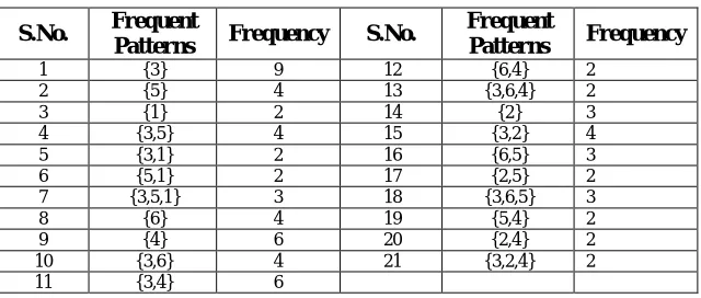
The set of all frequent patterns generated from the above HGmodel is given in the Table 4. Here the
minimum support is assumed as s = 20% .
C L
E
E
i
S Sj
) ( ) (Sj f Ei
f
) (SjL
) (SjC
) ) ( (f Sj s
)} ( : {Sj f Sj L
L
)} ( : {Sj f Sj C
C
) (Sj f
) ) (
(f Sj s
)} ( : {Sj f Sj L
L
)} ( : {Sj f Sj
C C
Table 4 Frequent patterns generated from the HGmodel in Figure .4 with s=20% S.No. Frequent
Patterns Frequency S.No.
Frequent
Patterns Frequency
1 {3} 9 12 {6,4} 2 2 {5} 4 13 {3,6,4} 2 3 {1} 2 14 {2} 3 4 {3,5} 4 15 {3,2} 4 5 {3,1} 2 16 {6,5} 3 6 {5,1} 2 17 {2,5} 2 7 {3,5,1} 3 18 {3,6,5} 3 8 {6} 4 19 {5,4} 2 9 {4} 6 20 {2,4} 2 10 {3,6} 4 21 {3,2,4} 2 11 {3,4} 6
Strong association rules can be generated from the set of frequent patterns mined from the given TDB. An association rule which satisfies both minimum support threshold and minimum confidence threshold is called a strong
association rule. For each frequent pattern X and for each nonempty proper subset Y of X the algorithm computes the
support and confidence of the association rule Y ⇒ X − Y.
For example from Table 4, X = {3, 6, 5} is a frequent pattern with frequency 3. The set of all association rules
generated from this pattern with the confidence and support for each rule is given in Table 5. The minimum confidence
threshold c and the minimum support threshold s are taken as 75% and 20% respectively.
Table 5 Association rules mined from the frequent pattern {3, 6, 5}.
Sl.No. Association Rules Confidence
of the Rule
Support of the Rule
R / R’
1 33 % 33 % R’
2 75 % 33 % R
3 75 % 33 % R
4 75 % 33 % R
5 75 % 33 % R
6 100 33 % R
For the TDB given in Table 3 of the disease dataset, 21 frequent patterns are generated. The number of frequent
patterns generated with various support counts is given in Table 4. Various association rules generated from the
frequent items set {3, 6, 5} is given in Table 5. One of the association rules is [cofidence=100,
support=30 %], the infromation that the patient who is suffering from the disease Fever and Head ache also tend to have the disease Cold. A support of 33 % for association rule means that 33% of all the patients under analysis suffering from the diseases Fever, Head ache and Cold together. A confidence of 100% means that 100% of patients suffering from Fever and Head ache also suffer from Cold. The number of association rules generated from the above disease data set is 51.
VI. RESULTS AND DISCUSSION
For the experimental purpose we have used datasets of different applications. These datasets were obtained from UCI repository of machine learning databases (http:\\www.ics.uci.edu/mlearn/MLRepository.html-1998). The characteristics of the datasets selected for the experiment are given in Table 6.
Table 6 Data sets used in the analysis Files Number of
Records
Number of Columns Adult.D14.N48842.C2.num 48842 14 Hepatitis.D19.N155.C2.num 155 19 Heart.D75.N303.C5.num 303 75 Census 48842 14 LetRecog.D106.N20000.C26.num 20000 17 MushroomD.90.N81424.C2.num 8124 23
To study the strategies we have conducted several experiments on a variety of data of different sizes and comparing our approach with the well-known SaM algorithms, and FI- tree algorithm. The performance metrics in the experiments is the total execution time taken and the support count for adult, hepatitis and heart datasets. For this comparison also same datasets were selected as for the above experiment with 30% to 70% of minimum support threshold. The experiments were conducted on 2.6 GHz CPU machine with 3 Gbytes of memory using Windows XP operating system. Time needed to mine frequent itemset for different algorithms using the data set given in Table 6 is discussed below.
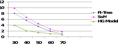
Table 7 Time scalability with respect to support on the Adult dataset Support in
%
Time in seconds
FI-Tree SaM HG model 30 8.12 9.85 4.03 40 5.69 6.72 2.08 50 3.56 4.51 1.5 60 1.99 2.69 1.1 70 1.01 1.7 0.8
Time taken to mine frequent pattern with various support threshold on Adult data set is given in the Table 7. The total execution time for our HG model is very much less than that of FI-Tree and SaM methods[9]. The SaM algorithm and FI-Tree algorithms take more time see Figure 6 as that compared to our approach.
Figure 6 Time scalability with respect to support on the Adult dataset
The total execution time for our new approach HG model and the other algorithms FI-Tree and SaM on Heart data set given in Table 8, algorithms large reduces with the increase in support threshold from 30% to 70%. Our proposed approach takes less time as that compared to the other two algorithms Sam and FI-Tree[7][8]. The execution time of HG model approach with SaM algorithms for hepatitis data set is given in Table 9
Table 8 Run time comparisons on Heart data set
Support in % Time in seconds
FI-Tree SaM HG model
30 0.05 0.07 0.035 40 0.4 0.06 0.031 50 0.3 0.05 0.028 60 0.03 0.03 0.02 70 0.01 0.02 0.009
Table 9 Run time comparisons on Hepatitis Data set
Support in % Time in seconds
FI-Tree SaM HG model
30 0.64 0.91 0.538
40 0.09 0.28 0.08
50 0.04 0.06 0.03
60 0.03 0.04 0.028
70 0.00 0.0 0.0
A detailed analysis to assess the performance of the algorithm HG- Model with respect to other frequent itemset mining algorithms is conducted. The performance matrix in the experiments is the total execution time taken and the number of item sets generated for different data sets[5][6]. The following performance analysis graphs Figure 7 shows
0 2 4 6 8 10 12
30 40 50 60 70
the execution time for the algorithms FP-Growth, Eclat, Relim, SaM with the new approach HG Model. Figure 8 shows performance analysis of our approach with other methods. This shows our method outperforms the others approaches.
Figure 7 Comparison of execution time of the algorithms on Adult data set. Figure 8 Performance analysis on Census data set
VII.CONCLUSION
In this paper a new data structure consisting of a hypergraph D is proposed for representing a TDB. Algorithms
for constructing D, generating frequent patterns using D and for generating frequent subhpergraphs are presented. During the entire process the database is scanned exactly once. Several types of experiments to test the effect of changing the support, transaction size, dimension, transaction length and use of other hypergraph theoretic parameters
are conducted to extract new knowledge about the TDB[9]. The comparison of the performance of this algorithm with
other existing algorithms in the literature using real data set are also studied and analyzed.
REFERENCES
[1] Berge C, Graphs and Hypergraphs. North-Holland, 1973.
[2] S. Arumugam and Sabeen S, “Association rule mining using path systems in directed graphs” INT J COMPUT COMMUN, ISSN 1841-9836, 8(6):791-799, December, 2013.
[3] S.Sabeen,” Classification of Messages in Dynamic Notice Board using Android” , European Journal of cientific Research ISSN 1450-216X Vol. 92 No 4, pp.496-509, December, 2012.
[4] Keyun Hu, Yuchang Lu, Lizhu Zhon, and Chungi Shi: Integrating classification and association rul mining: A concept lattice framework. In RSFDGrC’99: Proceeding of the 7th International Workshop on New Directions in Rough Sets, Data mining and Granular-soft Computing, pages 443-447, London, UK, Springer Verlag ISBN 3-540-66645-1, 1999.
[5] Maurice Houtsma and Arun Swami. Set-oriented mining of association rules. Research Report RJ 9567, IBM Almaden Research Center, San Jose, California, October 1993.
[6] Ozden. B, Ramaswamy S., and Silberschatz A. Cyclic association rules. In Proc. 1998 Int. Conf. Data Engineering (ICDE’98), pages 412– 421, Orlando, FL, Feb. 1998.
[7] HU. J, Max Donald A.H. and Mckay B.D., Physi. Rev. B.49.15263, 1994
[8] Han J. and Kamber M, Data minining, Concepts and Techniques second edition, 2010
[9] Borgelt C, SaM: Simple Algorithms for Frequent Item SetMining, IFSA/EUSFLAT 2009 conference, 2009.
[10] Agrawal R, Imielinski. T and Swami A., Mining Association Rules Between Sets Of Items In Large Database, In Proc. of the ACM SIGMOD International Conference on Management of Data (ACM SIGMOD 93), Washington, USA, 207-216, May 1993.
[11] Keyun Hu, Yuchang Lu, Lizhu Zhon, and Chungi Shi: Integrating classification and association rul mining: A concept lattice framework. In RSFDGrC’99: Proceeding of the 7th International Workshop on New Directions in Rough Sets, Data mining and Granular-soft Computing, pages 443-447, London, UK, Springer Verlag ISBN 3-540-66645-1, 1999.
[12] Walter A Kosters, Elena Marchiori, and Ard A.J. Oerlemans. Mining Clusters with association rules. In IDA'98 proceeding of the third international symposium on Advances in Intelligent Data Analysis, pages 39-50, London, UK.Springer Verlag ISBN 3-540-66332-0, 1999.
[13] Yew-Kwong Woon, Wee-Keong Ng, and Ee-Peng Lim. Online and Incremental mining of separately -grouped web access logs. In WISE'02: proceedings of the third international Conference on Web Information System Engineering, pages 53-62, Washington, DC,USA, IEEE Computer Society. ISBN 0-7695-1766-8, 2002.
[14] Mobasher B., Jain N., Han E., and Srinivatsava J., Webmining: Pattern Discovery from World Wide Web transactions. Tenchnical Report TR-96050, Department of Computer Science, University of Minnesota, 1996.
0 0.1 0.2 0.3 0.4 0.5 0.6
30 40 50 60 70
Ti
m
e
i
n
S
e
c
o
n
d
s
Support %
FP grow th Eclat
0 0.2 0.4 0.6 0.8 1 1.2 1.4
30 40 50 60 70
Ti
m
e
i
n
s
e
c
o
n
d
s
Support %
FP growth
Eclat
Relim
SaM
BIOGRAPHY
Dr. S. Sabeen is born on 18th May, 1976 at Parasuvaikal Village, Thiruvanathapuram district, Kerala, India. He