Evaluation of Source, Path and Site Effects by an Inversion of S-wave Spectra

(1)

Evaluation of Source, Path, and Site Effects by an Inversion of S-wave Spectra

Tetsushi Kurita1)_{, Satoru Takahashi}2)_{, and Masayoshi Shimada}2)

1) Seismic Engineering Department, Tokyo Electric Power Service Co., Ltd., Tokyo, Japan 2) Power Engineering R&D Center, Tokyo Electric Power Company, Yokohama, Japan

ABSTRACT

In this paper, source, path, and site effects are separated using historical earthquake data recorded near the prefectural boundaries of Shizuoka, Kanagawa, and Yamanashi in Japan. The constrained inversion analysis of S-wave spectrum is used to separate the effects. The seismic source spectrum obtained as a result of the inversion corresponds well to the theoretical

value obtained by the ω-2_{model, suggesting the validity of this analytical approach. Moreover, the Q-value, or the}

characteristics of the propagation path, was found to be close to the value for the Kanto region. In addition, the site effect corresponding to the amplification characteristics estimated from ground data for each site was obtained.

INTRODUCTION

The historical seismic data for a site consists of the source, path, and the site effects. In this study, these components were separated on the basis of records of earthquakes that have occurred near the boundaries of the three prefectures of Shizuoka, Kanagawa, and Yamanashi. The Philippine Sea plate and the Eurasian plate meet in this region, making the area seismically active. Earthquake observation stations operated by the Tokyo Electric Power Company (TEPCO) are found in the target region, and their data has been compiled into a database. Also found there are seismographic data compiled by other organizations. The goal of this study was to improve the accuracy of seismic motion prediction in the target points in order to evaluate the seismic motion characteristics of a broad area, including the observation sites.

BASIC INFORMATION

Observation Sites

For this study, station density was improved by incorporating K-NET (Kyoshin net) sites installed by the National Research Institute for Earth Science and Disaster Prevention (NIED) within the network of seismic observation posts operated by the Tokyo Electric Power Company (the TEPCO network). In the analysis of the seismic ground motion, the data of K-NET is excellent in benefit and convenience. The position (latitude and longitude information) is provided by GPS. In addition, ground data such as density, Vs, and Vp are disclosed. The position of each observation site is shown in Figure 1, indicated by solid circles. The large circle in the figure encloses the entire within a 40km radius of the TPC001 site. The stations are distributed almost uniformly around the periphery of this circle.

Earthquakes

The distribution of the epicenters of the object earthquakes is shown in Figure 1 as well. Epicenters concentrated on the vicinity of the center of the large circle. The list of earthquakes used for analysis is shown in Table 1. Here, the earthquakes

analyzed were selected according to a standard by which a maximum acceleration of 10cm/s2_{or more was observed.}

Moreover, the data after 1996 when the observation of K-NET started was used. In this examination, ten earthquakes were selected for the analysis. Almost earthquakes such as theYamanashi-ken Tobu Earthquake occurred along the prefectural boundaries of Shizuoka, Kanagawa, and Yamanashi. These earthquakes occurred shallower than 23km. Magnitudes are about 3-4. Seismic moment and moment magnitude (Mw) provided in the table were determined by FREESIA (Fundamental Research on Earthquakes and Earth’S Interior Anomalies) of NIED.

(2)

Figure 1. Location of stations (solid circles) and epicenters (open squares)

Table 2. List of earthquakes used in inversion

Origin Time Epicenter (degree)

No.

Y/M/D H:M Latitude Longitude

Depth

(km) Mj

Seismic Moment

(dyn･cm) Mw

1 96/07/18 19:55 35.4717 138.9650 20 3.5 －－

2 96/08/09 03:16 35.5067 138.9700 21 4.4 －－

3 96/10/25 12:25 35.4517 139.0050 23 4.5 －－

4 96/10/25 21:06 35.4717 138.9733 18 4.0 －－

5 97/06/08 18:35 35.4683 139.0217 13 3.6 2.42×1021 _3.6

6 97/09/24 07:02 35.5433 139.0100 20 4.2 6.39×1021 _3.8

7 97/11/04 10:31 35.2480 139.1157 15 4.0 1.21×1022 _4.0

8 98/09/25 04:49 35.4230 139.0173 15 3.3 －－

9 98/12/19 11:09 35.4187 138.9340 22 3.6 3.78×1021 _3.7

10 99/05/22 09:48 35.4497 139.1943 23 4.1 1.61×1022 _4.1

40km

YMN003 YMN006

YMN002

KNG011

KNG014

SZO011 SZO010

SZO009

SZO008

SZO001 KNG012

KNG013 TPC007 TPC006

TPC008 TPC003

TPC005 TPC001 TPC002

Yamanashi Pref.

Kanagawa Pref.

Shizuoka Pref.

TPC004

Tokyo Met.

139°00’ E 35°00’ N

3 4 5 6 7 0 30

60 30 60 100

Depth (km) 2

(3)

SEPARATION OF SOURCE, PATH, AND SITE EFFECTS

In general, observed seismic ground motion consists of source, path, and site effects. These factors must be separated in order to grasp the characteristics of seismic ground motion. After the factors separated, they can be evaluated individually. In this study, the three factors mentioned above were isolated from the earthquake record using the inversion analysis in order to grasp the seismic ground motion characteristics around the prefectural boundaries of Shizuoka, Kanagawa, and Yamanashi.

Inversion Method

The inversion method proposed by Iwata and Irikura [1] was used. The S-wave part of the seismic wave observed in far

field is assumed. The S-wave may be expressed as the linear combination of source, path, and site effects. For I earthquakes

and J stations, seismic wave spectra (Fourier amplitude spectral density) of

i

-th earthquake at

j

-th station is:

×

_ççè

æ

-

×

_×

×

_÷÷ø

ö

×

=

-S S

ij j

i ij ij

V

Q

R

f

g

f

s

R

f

o

1

exp

F

(1)

where

s

_i

f

is the source spectrum of the

i

-th earthquake;

g

_j

f

the local site effect near the

j

-th station;

R

_ij the

hypocentral distance between the

i

-th earthquake and the

j

-th station;

V

_S the average S-wave velocity of the path; and

S

Q

the average quality factor of the propagation path for the S-wave. This model makes two assumptions. First, neither the

directivity nor the radiation pattern of the source are considered. Second, the

Q

_S-value does not depend on the path. The

following normalization of the geometrical attenuation is performed for equation (1) for linearization.

ij

ref ij

ij

f

R

o

=

/

(2)

where

R

ref is the arbitrary normalized distance. After the geometrical attenuation is corrected, linearization can be

performed by taking the logarithm of both sides of Eq. (1).

S S

ij j

i ref

ij

R

s

g

e

f

R

Q

V

o

=

-

log

+

log

+

log

-

(log

)

×

/

×

log

F

(3)

where,

e

is Napier’s number. Equation (3) becomes a simultaneous equation composed of the equation of the maximum I ×

J piece by the combination of the earthquakes and the stations. This becomes a least squares problem in which the I seismic

source spectra of the earthquakes, the J station characteristics, and a

Q

_S-value for each frequency are determined by these

simultaneous equations. The variables must satisfy the following condition if Eq. (3) is to have a solution.

1 +

+

³

´

J

I

J

I

(4)

Eq. (3) may be solved by singular value decomposition. The trade-off arises between the seismic source spectrum and the

station spectrum when Eq. (3) is solved directly, and no correct answers other than the

Q

_S-value are obtained. A suitable

constraint is required to prevent it. Iwata and Irikura [1988] provided the following constraint: the station spectrum in each

station must be two or greater.

2 ³

f

g

_j (5)

(4)

Preparation of Data Set

First, the S-wave part was taken out by using the time window from the time history of the acceleration record. The cosine taper of 10% at the duration of the window was applied to both ends of the time window. The duration of the time window has been changed in proportion to the magnitude of each earthquake. Following FFT, the average of the spectra of two horizontal elements was calculated. This processing is intended to keep the validity of the assumption (above-mentioned) to ignore the directivity of the source. The following processing was smoothing the spectrum. A steady spectrum made it possible to set 1.0Hz to 10Hz as an analytical frequency band. The frequency band was divided into ten even segments on the logarithmic axis.

n

f

n

=

´

-1

10 log

,

n

=

1 ,

2 ,

L

,

10

(6)

These frequencies (fn) made the representative points. The representative value of the Fourier spectrum is obtained from the

arithmetical average values of data before and behind that. The averaging width was set to 0.1 on the logarithmic axis. Similar processing was performed for all records, and 112 data sets were made. The number of observation equations obtained is 112, while the number of unknown parameters is given by (earthquakes:10) + (Q-value:1) + (observation sites:20) = 31, thereby providing solutions to this equation.

Results

It is necessary to give the average S-wave velocity of the earth's crust in the inversion. As an approximate value, Vs=3.7km/s was assumed. The inversion results are shown as follows.

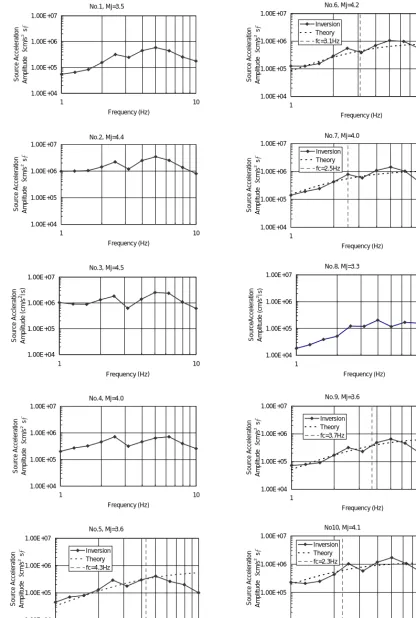
Seismic source spectra

The inversion results of the seismic source spectra (thick solid lines) are shown in Figure 2. The inversion results of all seismic source spectra display the tendency for amplitude to decrease by the high frequency side. Similar tendencies have already been reported for the analytical results of previous study. The constraint (it is twice or more as for the site effect) is thought to influence this phenomenon [1], [6]. Therefore, it is not possible to judge it at once of being able to observe the

cut-off frequency (fmax) in these spectral shapes. Moreover, the tendency for amplitudes of seismic source spectrums to increase

appears clearly as the JMA magnitude increases. As mentioned above, it appears that the result obtained does not result in contradictions. The seismic moments are obtained from focal mechanism analysis by FREESIA of NIED for five earthquakes.

In addition, Takemura et al. [7] proposes the following relationship between seismic moment (M0) and corner frequency (fc).

28 .

23 log

3 log

M

₀

=

-

f

_c

+

(7)

The corner frequency can be calculated by using Eq. (7). The values calculated for fc are shown in Figure 2 by a thin broken

line. The theoretical seismic source spectra (thick broken line) obtained from the ω-2_{model [8] are also shown in this figure.}

These theoretical spectra are calculated by substituting the seismic moments and the corner frequencies for Eq. (8).

2 2 0

3

1

2

4 ÷÷ø

ö

ççè

æ

+

×

=

c i d

i

f

M

Vs

R

f

s

F

H

F

(8)

Here, general values were assumed for unknown parameters. The radiation coefficient is Rd=0.63, the average density of the

earth's crust is ρ=2.7g/cm3_{, and an average S-wave velocity of the earth's crust is}_Vs_{=3.7km/s. The inversion results of the}

seismic source spectra are in good agreement with the theoretical values calculated from the ω-2_{model, confirming the}

(5)

No.1, Mj=3.5 1.00E+04 1.00E+05 1.00E+06 1.00E+07 1 10 Frequency (Hz) So u rce Acce le ra ti o n A m plit ude 　（ cm/ s 2・ s ） No.6, Mj=4.2 1.00E+04 1.00E+05 1.00E+06 1.00E+07 1 10 Frequency (Hz) So u rce Acce le ra ti o n A m plit ude 　（ cm/ s 2・ s ） Inversion Theory fc=3.1Hz No.2, Mj=4.4 1.00E+04 1.00E+05 1.00E+06 1.00E+07 1 10 Frequency (Hz) So u rce Acce le ra ti o n A m plit ude 　（ cm/ s 2・ s ） No.7, Mj=4.0 1.00E+04 1.00E+05 1.00E+06 1.00E+07 1 10 Frequency (Hz) So u rce Acce le ra ti o n A m plit ude 　（ cm/ s 2・ s

） Inversion_Theory

fc=2.5Hz No.3, Mj=4.5 1.00E+04 1.00E+05 1.00E+06 1.00E+07 1 10 Frequency (Hz) S our ce A ccler ation A m plitude ( c m/s 2･ s) No.8, Mj=3.3 1.00E+04 1.00E+05 1.00E+06 1.00E+07 1 10 Frequency (Hz) So u rce Acce le ra ti o n A m plit ude ( c m /s 2･ s) No.4, Mj=4.0 1.00E+04 1.00E+05 1.00E+06 1.00E+07 1 10 Frequency (Hz) So u rce Acce le ra ti o n A m plit ude 　（ cm/ s 2・ s ） No.9, Mj=3.6 1.00E+04 1.00E+05 1.00E+06 1.00E+07 1 10 Frequency (Hz) So u rce Acce le ra ti o n A m plit ude 　（ cm/ s 2・ s ） Inversion Theory fc=3.7Hz No.5, Mj=3.6 1.00E+04 1.00E+05 1.00E+06 1.00E+07 1 10 Frequency (Hz) So u rce Acce le ra ti o n A m plit ude 　（ cm/ s 2・ s ） Inversion Theory fc=4.3Hz No10, Mj=4.1 1.00E+04 1.00E+05 1.00E+06 1.00E+07 1 10 Frequency (Hz) So u rce Acce le ra ti o n A m plit ude 　（ cm/ s 2・ s

） Inversion_Theory

fc=2.3Hz

(6)

Q-value of propagation path

The inversion result of the Q-value is shown in Figure 3. It is clear that the obtained Q-value depends on frequency. The regression formula for the inversion result is shown in this figure. The involution term expresses the inclination of the straight line. The involution term obtained is greater than a general value. However, it appears that an appropriate value is obtained close to 1.0.

A comparison between the average Q-value in the Kanto region obtained for the previous studies [4], [9] and the inversion result of this study is shown in Figure 4. The result of this study is a large value on the low-frequency side compared with the research results of previous studies. However, virtually no difference is seen on the high-frequency side. Such tendencies indicate a strong frequency dependence on the regression formula. Due to the small magnitudes represented by the data used here (around 3 to 4), the difference on the low-frequency side may be discussed without precise values. Future clarification will require extensive data concerning large magnitudes. The difference between the results of this study

and the results of the previous examination in terms of overall tendency are not necessarily large. The average QS obtained in

this study is relatively close to an average Q-value for the Kanto district.

1/Q = 0.0246f-1.2147 R2 = 0.8747

0.0001 0.0010 0.0100 0.1000

1 10

Frequency (Hz)

1/

Q

0.0001 0.0010 0.0100 0.1000

1 10

Frequency (Hz)

1/Q

This Study Aki (1980) Kinoshita (1994) Kato et al. (1996) Nakayama et al. (1998)

Figure 3. Inversion result of Q-value Figure 4. Comparison of Q-values of this study and previous studies

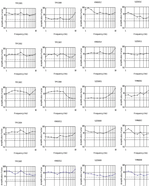
Site effects

The site effects reflect amplification factors for shallower ground than seismic bedrock. Inversion results of site effects are shown in Figure 5. In this figure, the short broken line indicates the amplification factor of 2.0, assumed to be a constraint. When the site effects of TPC001 and TPC002 located in the same site are compared, the shape of them is very similar, making the site effects of them nearly identical. In addition, there is a feature where the peak appears in about 3Hz of the spectrum.

All amplification factors are large, despite the locations within mountainous area for TPC003, TPC007, and TPC008. Topographic effects apparently influence the amplification factor, since these points are located in the inclination ground, the valley, and the cliff geographical features.

Because TPC004 and TPC005 are located in the plains, the amplification factors are very large compared to the other points.

TPC006 is located in a mountainous area, and the overall amplification factor is small. The soil-structure of this point is unclear.

(7)

T P C 0 0 1 0.1 1 10 100 1 10

F r e q u e n c y ( H z )

Am

p

lification Factor

T P C 0 0 6

0.1 1 10 100

1 10

Am

p

lification F

a

ctor

K N G 0 1 3

0.1 1 10 100

1 10

Am

p

lification Factor

S Z O 0 1 0

0.1 1 10 100

1 10

Am p lifi cat io n F acto r

T P C 0 0 2

0.1 1 10 100

1 10

Am p lif ic at ion Fact or

T P C 0 0 7

0.1 1 10 100

1 10

K N G 0 1 4

0.1 1 10 100

1 10

S Z O 0 1 1

0.1 1 10 100

1 10

Am

p

lification Factor

T P C 0 0 3

0.1 1 10 100

1 10

Am

p

lification Factor

T P C 0 0 8

0.1 1 10 100

1 10

S Z O 0 0 1

0.1 1 10 100

1 10

Am p lifi cat io n f acto r

Y M N 0 0 2

0.1 1 10 100

1 10

T P C 0 0 4

0.1 1 10 100

1 10

Am p lif ic at ion Fact or

K N G 0 1 1

0.1 1 10 100

1 10

Am

p

lification Factor

S Z O 0 0 8

0.1 1 10 100

1 10

Y M N 0 0 3

0.1 1 10 100

1 10

Am

p

lification Factor

T P C 0 0 5

0.1 1 10 100 1000 1 10

K N G 0 1 2

0.1 1 10 100

1 10

S Z O 0 0 9

0.1 1 10 100

1 10

Y M N 0 0 6

0.1 1 10 100

1 10

(8)

CONCLUSIONS

In this paper, earthquake records were analyzed to clarify seismic ground motion characteristics near prefectural boundaries of Shizuoka, Kanagawa, and Yamanashi in Japan. The characteristics of this region were evaluated using the acceleration records of the TEPCO network and K-NET.

The conclusions obtained in this study are given below.

1) Source, path, and site effects were separated on the basis of seismic records, using the method of inversion analysis of the

S-wave spectra proposed by Iwata and Irikura [1].

2) Since seismic source spectra obtained by inversion appear to agree in amplitudes, corner frequencies, and magnitudes, the

result appears to be correct.

3) The clear frequency dependence of the Q-value was observed. The obtained Q-value is close to the results obtained in past

research in the Kanto district.

4) The site effects from the inversion are accorded with that estimated from the ground data.

ACKNOWLEDGMENT

A portion of the data used in this analysis was povided by K-NET. This data has been placed in the public domain by the National Research Institute for Earth Science and Disaster Prevention. The authors would like to express their gratitude for the availability of this data.

REFERENCES

1. Iwata, T. and Irikura, K., “Source parameters of the 1983 Japan sea earthquake sequence”, J. Phys. Earth, 36, 1988,

pp.155-184.

2. Kato, K., Takemura, M., Ikeura, T., Urao, K. and Uetake, T., “Preliminary analysis for evaluation of local site effects

from strong motion spectra by an inversion methods”, J. Phys. Earth, 40, 1992, pp.175-191.

3. Takemura, M., Kato, K., Ikeura, T. and Shima, E., “Site amplification of S-wave from strong motion records in special

relation to surface geology”, J. Phys. Earth, 39, 1991, pp.537-552.

4. Yamanaka, H., Nakamaru, A., Kurita, K. and Seo, K., “Evaluation of site effects by an inversion of S-wave spectra with a

constraint condition considering effects of shallow weathered layers”, Zisin, Second Series, Vol.51, 1998, pp.193-202. (in Japanese)

5. Lawson, C. L. and Hanson, R. J., “Solving Least Squares Problems”, Prentice-Hall, Inc., Englewood Cliffs, New Jersey,

1974.

6. Maeda, T. and Sasatani, T., “A study of source, path and site effects by using strong motion data from intermediate-depth

events”, Proceedings of the Forth Toshi-chokka Jishin Saigai Sogo Symposium, 1999, pp.115-118. (in Japanese)

7. Takemura, M., Ikeura, T. and Uetake, T., “Characteristics of source spectra of moderate earthquakes in a subduction zone

along the Pacific coast of the southern Tohoku district, Japan”, J. Phys. Earth, 41, 1993, pp.1-19.

8. Boor, D. M., “Stochastic simulation of high-frequency ground motions based on seismological models of the radiated

spectra”, Bulletin of the Seismological Society of America, Vol. 73, No.6, 1983, pp.1865-1894.

9. Kinoshita, S. “Frequency-dependent attenuation of shear waves in the crust of southern Kanto area, Japan”, Bulletin of