Proactive and Efficient Spare Parts Inventory Management Policies Considering Reliability Issues

(1)

University of Windsor University of Windsor

Scholarship at UWindsor

Electronic Theses and Dissertations Theses, Dissertations, and Major Papers

2013

Proactive and Efficient Spare Parts Inventory Management

Policies Considering Reliability Issues

Jingyao Gu

University of Windsor

Follow this and additional works at: https://scholar.uwindsor.ca/etd

Part of the Engineering Commons

Recommended Citation Recommended Citation

Gu, Jingyao, "Proactive and Efficient Spare Parts Inventory Management Policies Considering Reliability Issues" (2013). Electronic Theses and Dissertations. 4888.

https://scholar.uwindsor.ca/etd/4888

(2)

Proactive and Efficient Spare Parts Inventory

Management Policies Considering Reliability Issues

by

Jingyao Gu

A Thesis

Submitted to the Faculty of Graduate Studies

through the Department of Industrial and Manufacturing Systems Engineering in Partial Fulfillment of the Requirements for

the Degree of Master of Applied Science at the University of Windsor

Windsor, Ontario, Canada 2013

(3)

Proactive and Efficient Spare Parts Inventory

Management Policies Considering Reliability Issues

by

Jingyao Gu

APPROVED BY:

_______________________________________________________ Dr. Xiaolei Guo

Odette School of Business

_______________________________________________________ Dr. Zbigniew Pasek

Department of Industrial and Manufacturing System Engineering

_______________________________________________________ Dr. Guoqing Zhang, Co-Advisor

_______________________________________________________ Dr. Kevin Li, Co-Advisor

Odette School of Business

_______________________________________________________ Dr. Reza Lashkari, Chair of Defense

(4)

AUTHOR’S DECLARATION OF ORIGINALITY

I hereby certify that I am the sole author of this thesis and that no part of this thesis has been published or submitted for publication.

I certify that, to the best of my knowledge, my thesis does not infringe upon anyone’s copyright nor violate any proprietary rights and that any ideas, techniques, quotations, or any other material from the work of other people included in my thesis, published or otherwise, are fully acknowledged in accordance with the standard referencing practices. Furthermore, to the extent that I have included copyrighted material that surpasses the bounds of fair dealing within the meaning of the Canada Copyright Act, I certify that I have obtained a written permission from the copyright owner(s) to include such material(s) in my thesis and have included copies of such copyright clearances to my appendix.

(5)

ABSTRACT

(6)

ACKNOWLEDGMENT

I would like to express my deepest gratitude to my supervisors, Dr. Guoqing Zhang, and Dr. Kevin Li, for their devoted guidance, immense support and constant encouragement during my graduate study in Windsor. Without their excellent mentoring skills and professional knowledge, this work would not have been done. I will eternally remember this life-changing experience to work with them.

I would also like to convey my heartiest appreciation to Dr. Zbigniew Pasek and Dr. Xiaolei Guo for being on my advisory committee and providing valuable suggestions on my work.

(7)

LIST OF FIGURES

Figure 1. Time sequence ... 16

Figure 2．Cost vs. parts arrival time for main gearbox when Q=37.90 ... 24

Figure 3．Cost vs. order quantity for gearbox when =143.52 ... 25

Figure 4. Cost vs. parts arrival time for main gearbox when Q=25.52 ... 27

Figure 5. Cost vs. order quantity for gearbox when =1170.03 ... 27

Figure 6. Total cost as increases ... 30

Figure 7. Optimal order quantity as increases ... 30

Figure 8. Optimal inventory replenishment time as increases ... 30

Figure 21. The flowchart of the combination of Lagrangian heuristic and iteration method . 55 Figure 22. Order quantities change when K increases ... 62

Figure 23. Parts arrival times change when K increases ... 62

Figure 24. Expected total cost changes when K increases ... 62

Figure 25. Order quantities change when increases ... 64

Figure 26. Parts arrival times change when increases ... 64

Figure 27. Expected total cost changes when increases ... 64

Figure 28. Order quantities change when increases ... 65

Figure 29. Parts arrival times change when increases ... 66

(10)

LIST OF TABLES

Table 1．Definitions of Rotables, Repairables, Expendables and Consumables ... 8

Table 2. Parameter values of main gearbox in Deshpande et al. (2006)... 22

Table 3. New designed parameter values for main gearbox ... 22

Table 4．Results from iterative and GAMS solution approaches ... 24

Table 5. Representative points in Figure 1 and Figure 2 ... 25

Table 6. Modified parameter values ... 26

Table 7. Calculation results for modified parameter values... 26

Table 8. Representative points in Figure 4 and Figure 5 ... 27

Table 9．Objective values comparison of two models when changes ... 29

Table 10. Objective values comparison of two models when changes ... 31

Table 11. Objective values comparison of two models when changes ... 33

Table 12. Objective values comparison of two models when changes... 34

Table 13. Objective values comparison of two models when n changes ... 36

Table 14. Parameter values for two PNs example ... 57

Table 15. Calculation results and comparison for two PNs example ... 57

Table 16. Calculation results and comparison for the problem with m=10 ... 58

Table 17. Test Problem sizes, solutions, relative gap, and running time ... 59

Table 18. Basic values of parameters ... 60

Table 19. Decision variables and objective value change when K increases... 60

Table 20. Decision variables and objective value change when increases ... 63

(11)

CHAPTER 1: INTRODUCTION

1.1 General Overview

Spare parts inventory management plays an important role in many industries, such as airline, trucking, and manufacturing industries. Spare parts are interchangeable parts that are kept in an inventory and used for the repair or replacement of failed parts. The problem of offering an adequate yet efficient supply of spare parts, in support of maintenance and repair of aircraft, trucks, plant and equipment, is an especially vexing inventory management scenario. Most spare parts are very expensive and costly to keep in stock. However, they must be on hand once needed due to high cost of flight cancellation, logistics interruption or plant shutdown.

(12)

help keep aircraft, trucks, equipment and plant in an operating condition. Furthermore, WIP and final product inventories can be adjusted by changing production rates, and expediting delivery. However, spare parts inventory levels are mainly determined by how equipment or vehicles are used and how they are maintained. In addition, the spare parts shortage costs are usually very high and sometimes not easy to gauge. Because maintenance parts stockouts may not only lead to significant production losses, but also intangible cost such as increased risk to operating personnel. Finally, obsolescence may also be a problem for spare parts due to their specialized uses.

(13)

1.2 Proposed Research

1.2.1 Research Topic

Our research was motivated by creating an efficient spare parts inventory model to provide better service for maintenance needs. The objective of this research is to develop an effective approach to determine optimal spare part inventory policies with taking into account reliability issues. In details, this research involves:

1) Analyze the features of spare part inventory management problem with considering the failure and maintenance process. In our research, we take airline industry as an example but the approaches and results proposed are not limited to the industry. 2) Establish the mathematical models to help decision-makers to determine the best order time and the optimal order quantities so that the total cost, including purchasing, holding, and shortage costs, is minimal. The uncertainty on both the number of failures and the lifetime for each part is considered in the problem.

3) Consider both single spare part and multiple spare parts with a budget constraint. It is very common that there are lots of spare parts in an inventory system and the company usually faces budget constraint when making ordering decision for those multiple spare parts. Thus it is more practical to investigate inventory policies for multiple spare parts with a budget constraint.

(14)

are nonlinear programming problems or stochastic programming problems, and they are difficult to solve, especially for multiple Part Number case.

5) Make sensitivity analysis to compare different spare part ordering policies.

1.2.2 Organization of Thesis

This thesis is organized as follows. Chapter 2 describes two single part number (PN) models, a basic mathematical model and an improved mathematical model. The basic model assumes that the shortage period starts from mean time to failure (MTTF). Numerical and iterative methods as well as GAMS are employed to solve this model. The improved model takes into account accurate shortage time. Due to its complexity, only GAMS is applied in solution methodology. Both models are proved effective in cost reduction as reflected by numerical examples and their results. Comparisons of the two models are also discussed.

(15)

(16)

CHAPTER 2: EFFICIENT SPARE PARTS INVENTORY

MANAGEMENT FOR AIRCRAFT MAINTENANCE – SINGLE

PART NUMBER (PN) CASE

2.1 Introduction

In airline industries, an operator has to deal with two types of issues: the aircraft operating cost and customer satisfaction. Aircraft maintenance planning plays a major role in both of them. On the one hand, based on an analysis conducted by the International Air Transport Association (IATA)’s Maintenance Cost Task Force, the maintenance cost takes up about 13% of the total operating cost, and it can be reduced by a good planning. On the other hand, an excellent maintenance program can effectively avoid flight delays and cancellations, thus improve customer satisfaction and competitiveness in the industry. Spare parts inventories exist to serve the maintenance planning. An excess of spare parts inventory leads to a high holding cost and impedes cash flows, whereas inadequate spare parts can result in costly flight cancellations or delays with a negative impact on airline performance. Since the airline industry involves with a large number of parts and some of them are quite expensive, it is important to find an appropriate inventory model to achieve a right balance.

(17)

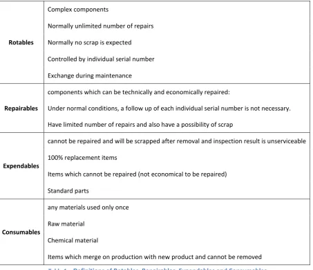
classified into four groups: Rotables, Repairables, Expendables and Consumables. For different categories, different replenishment policies are used. Rotables and Repairables are mainly based on predicted failures estimated by manufacturers, and the planning parameters are finished as management decision. As to Expendables and Consumbles, the reorder point system (ROP) is used and input comes from historical demand with estimated changes. However, this kind of inventory management is typically subjective and imprecise, thus is not an ideal policy. From a survey conducted by Ghobbar and Friend (2004), 152 out of 175 respondents were using the ROP system and about half were dissatisfied and considering implementing new systems.

(18)

previous inventory models that just address the problem of determining the amount of parts to be purchased, our efficient inventory model satisfies spare parts demands from two perspectives: quantity and time. Therefore, it can better improve service level and control the total costs which generally include purchasing cost, holding cost, and shortage cost.

Rotables

Complex components

Normally unlimited number of repairs

Normally no scrap is expected

Controlled by individual serial number

Exchange during maintenance

Repairables

components which can be technically and economically repaired:

Under normal conditions, a follow up of each individual serial number is not necessary.

Have limited number of repairs and also have a possibility of scrap

Expendables

cannot be repaired and will be scrapped after removal and inspection result is unserviceable

100% replacement items

Items which cannot be repaired (not economical to be repaired)

Standard parts

Consumables

any materials used only once

Raw material

Chemical material

Items which merge on production with new product and cannot be removed

Table 1．Definitions of Rotables, Repairables, Expendables and Consumables

(19)

triggered to reduce downtime caused by parts delivery time. In our analysis, we examine the parts failure distribution to find optimal order time and order quantity by considering that the lifetime and quantity of installed parts failure distribution may influence the duration and numbers of spare parts shortage or overstock, thus result to total cost fluctuation. A non-linear programming (NLP) model is presented with the objective of minimizing air carriers’ expected cost in spare parts. Numerical and iteration methods and GAMS are employed to solve the model.

This chapter is organized as follows. In the next section, we give a brief literature review. Section 2.3 presents a basic mathematical model considering shortage period starts from mean time to failure (MTTF). Numerical and iteration methods as well as GAMS can be used to solve this model. We also develop an improved mathematical model, which takes into account exact shortage time, and its solution methodology in Section 2.4. Section 2.5 illustrates the value of our models in cost reduction by numerical examples and their results. Sensitivity analysis and models comparison is conducted in the following section. Finally, section 2.7 provides the conclusions and suggestions for future research.

2.2 Literature Review

(20)

(21)

The most recent paper in this subject area is Wang (2012), who presents a model to optimize the order quantity, order intervals, and PM intervals jointly under a two-stage failure process. The aforesaid papers mainly address the problem either from an inventory point of view based on the past spare parts usages to forecast the future demand, or from a PM point of view to find an optimal order quantity and PM interval. In practice, spare parts demands are highly related with flying hours/landings. Due to the correlation between part aging and failures, impending high demands for a part might be forecasted even the current demand is low, which is counter to the traditional replenishment system that high demand triggers replenishment and low demand scales back replenishment. This partially explains why the forecasting methods based on historical data cannot be directly used for forecasting future demand in our case. Besides, PM inventory management is different from failure-based inventory management. To the author’s best knowledge, limited research handles failure-based procurement inventory management which is very common in practice. As the spare parts demand is uncertain, and sometimes the part delivery time may be very long, it could lead significant loss if a critical part fails but there is no spare to replace it.

(22)

(23)

2.3 Basic Mathematical Model and Solution Methodology

2.3.1 Basic Mathematical Model

In this chapter, we consider a generalized ordering policy for only one kind of part with a given part number (PN) in a single period. A part number is a fundamental identifier of a particular part design used in the airline industry. It unambiguously identifies a part design within a single corporation, or sometimes across several corporations. For example, when specifying a bolt, it is easier to refer to "PN BACB30LH3K24" than describing the key information of the bolt, such as dimensions, material, installed position and manufacturer, which may be lengthy and incomplete. Moreover, multiple parts with the same PN are often found in one or more aircrafts. For instance, if one Boeing 737-300 has installed 200 PN BACB30LH3K24 bolts, and the fleet size of Boeing 737-300 is 20, thus the total number of PN BACB30LH3K24 operated by the carrier will be 4000.

(24)

Input parameters and function:

the unit holding cost per unit time the unit shortage cost per unit time

planning horizon, can be infinite order lead time

demand quantity, a random variable unit cost

the PDF of failure distribution considering lifetime for each part

the PDF of failure distribution considering number of failures for each PN

the CDF of failure distribution considering lifetime for each part

the CDF of failure distribution considering number of failures for each PN

Define the following decision variables point in time to place an order the parts arrival time

order quantity

The objective of minimizing the expected total cost is formulated as:

Min R = ∫ [ ∫ ] ∫

[ ∫ ∫ ]

(1)

(25)

(26)

Figure 1. Time sequence

2.3.2 Solution Methodology

2.3.2.1 Numerical and iteration methods

From objective function (1), we are obviously interested in determining the value of and Q, which minimize the expected cost R. Without considering any constraint, Q and can be found by the following procedure:

[ ∫ ] [ ]

[ ∫ ∫ ]

(2)

It follows that

{ [ ∫ ]} for all Q

Because the second-order derivative is nonnegative, the function R (Q) is said to be convex. The optimal solution, Q*, occurs where

equals zero. That is,

[ ∫ ] [ ∫ ∫ ]

(27)

(3)

Also,

∫ [ ]

(4)

It follows that

for all Q

As the second-order derivative is nonnegative, R ( ) is convex, and the optimal solution, *, is attained when equals zero. That is,

∫

(5)

One of the widely-used probability distributions in reliability to model fatigue and wear-out phenomena is the normal distribution, as illustrated by the works of Deshpande et al. (2006), Muchiri and Smit (2011), Tuomas et al. (2001), Batchoun et al. (2002), Byington et al. (2002), and Kiyak (2012). If we assume that f(x) is normally distributed, with a mean and standard deviation , the formula for the PDF is

√ [

]

Meanwhile, assume g(z) follows a normal distribution with a mean and standard deviation . The formula for the PDF is

√ [

(28)

As the random variable ranges from to , the normal distribution is not a true reliability distribution. However, if for most observed values of mean and standard deviation in the context of this study, the probability that the random variable takes on negative values is negligible, then the normal distribution can be regarded as a reasonable approximation to a failure process. We assume , also f(x) and g(z) are uncorrelated.

From equation (3), we have

{ [ (

) (

)]

}

(6)

Here is the standard normal density function, and is the standard normal cumulative distribution function for the normal density function is the inverse of the cumulative density function for the normal density function .

_{ [

] [

]

}

(7)

Here is the standard normal density function, and is the standard normal cumulative distribution function for the normal density function . is the inverse of the cumulative density function for the normal density function .

(29)

algorithm is employed to find solutions. The algorithm converges in a finite number of iterations, provided that a feasible solution exists. The algorithm is described as follows:

Step 0. Use the initial solution

_{ [ (

) (

)]

} and let

Set i=1, and go to step i.

Step i. Use to determine from equation (7). If , stop; the optimal solution is , and . Otherwise, use in equation (6) to compute . Set i=i+1, and repeat step i.

When the iteration terminates, we can find the optimal timing to place an order as

.

From equation (1), the objective function can be reformulated as:

{ [ ] [ ]}

(8)

2.3.2.2 Solve the basic model by GAMS

(30)

CONOPT can yield good results. MINOS is suitable for large constrained problems with a linear or nonlinear objective function and a mixture of linear and nonlinear constraints. For nonlinear constraints, MINOS implements a sequential linearly constrained algorithm derived from the Robinson's method. CONOPT is a feasible path solver based on the generalized reduced gradient method and is often preferable for nonlinear models where feasibility is difficult to achieve.

2.4 An Improved Mathematical Model and Solution Methodology

In the basic model presented in the previous section, the value of T minus MTTF instead of the failure time is adopted to define the parts shortage period till the end of the planning horizon. The improved mathematical model herein aims to find when the failure occurs and plugs it into the model. Therefore, this improved model is designed to find more accurate order quantity Q and order time .

In reliability engineering, it is well known that given that where are n ordered failure times comprised in a random sample, the number of units surviving at time is n-i. A possible estimate for the reliability function can be expressed as

̂

The estimate for the cumulative failure distribution is

̂ ̂ .

(31)

technical information provided by the original equipment manufacturer (OEM), and is

the failure time. We also assume that f(x) is normally distributed, and the failure times follow , then

.

Because ̂( ) , and ( ) ,

we have

. That is, ( ).

Accordingly, the failure time can be expressed as

( ) ,

(9) and equation (1) can be improved as

Min R = ∫ [ ( ) ] ∫

[ ∫ ∫ ]

(32)

2.5 Numerical Examples and Results

A numerical example, which is introduced in Deshpande et al. (2006), is modified by introducing the distribution of the number of failures for a specified PN. The data are originally drawn from the aircraft maintenance and inventory databases of the United States Coast Guard (USCG) ( Deshpande et al., 2006). Here we list the same parameter values used in Deshpande et al. (2006) in Table 2, which is about the main gearbox of aircraft type HH65A.

Note that if we assume a daily flying time of 10 hours, the gearbox mean age at failure should be 2436/10=243.6 days, similarly the standard deviation should be 659/10=65.9 days. Additional parameter values in Table 3 are introduced for our new models.

Unit price Unit holding cost per day Unit shortage cost per day Mean time to failure Standard deviation

c h= 0.25*c/365 s=5*c/365

$449,586.00 $307.94 $6,158.71 2436 hours 659 hours

Table 2. Parameter values of main gearbox in Deshpande et al. (2006)

Planning horizon Mean number of failures Standard deviation Total number of parts observed in fleet

T n

5 years=1,825days 25 10 200

Table 3. New designed parameter values for main gearbox

(33)

the decision variables for both the Iterative approach and the GAMS approach produce very similar results. The objective function values for both approaches are slightly different with a percentage error margin of 0.45%. This error is likely due to the assumption that

∫ ∫ [ ] [ ] in the iterative approach, which

neglects the part of the negative values in the normal distribution. On the other hand, both approaches yield almost identical decision variable values. Next we compare the differences of GAMS results between the basic and improved models. The values of are essentially the same for the models. However, the values of Q and R change to a certain degree. Compared with the basic model, the value of Q for the improved model increases by 0.55%, and the value of R increases by 0.54%. A closer examination of the two objective functions reveals that the only difference exists in the second term: the shortage period described in the basic model is ( ), while in the improved model it is ( ) [

₍ ₎ _]_{. Because the change is only related to Q and R, it barely affects the optimal}

value of . In this example, is less than implying that the shortage situation starts a little earlier in the improved model than that in the basic model, therefore more shortage cost would be incurred and more spare parts should be ordered during the planning horizon.

(34)

comparable as illustrated in Table 4. Figure 2 illustrates the relationship between the expected cost and parts arrival time for the main gear box when Q=37.90. The optimal value of parts arrival time, which minimizes the expected cost, should be set at 143.52. Based on the trend, as the parts arrival time increases, the expected cost first decreases slightly, followed by a dramatic increase. The reason is that, compared with the shortage cost, the holding cost only takes a small fraction of the unit cost. Moreover, the mean age at failure happens at the early period of the planning horizon.

Solution approach Iterative GAMS

basic model basic model improved model

Objective function value R $30,110,394.24 $29,974,161.85 $30,135,359.75

Decision variable Q 37.90 37.92 38.13

143.52 143.41 143.48

* * 185.91

Iteration number 3 14 14

Feasible solution yes yes yes

Table 4．Results from iterative and GAMS solution approaches

Figure 2．Cost vs. parts arrival time for main gearbox when Q=37.90

0 50 100 150 200 250 300 350 400 450

0 500 1000 1500 2000

(35)

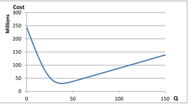
Figure 3 depicts the relationship between the expected cost and order quantity curve for the main gear box when =143.52. From the figure, we can find that as the order quantity increases, the expected cost drops sharply till Q= 37.90, then followed by a much slower gradual increase. The different slopes of the curve can be intuitively explained as follows: if the actual order quantity is below the optimal order quantity, compared with overstocking, the shortage cost is much higher than the holding cost.

Figure 3．Cost vs. order quantity for gearbox when =143.52

Decision variable Objective function value % Cost reduction Q Total cost R (R-Optimal value)/R

143.515 37.90 $30,110,394.24 Optimal value

0 0 $243,691,145.51 87.64%

143.515 0 $243,690,259.81 87.64%

143.515 150 $138,579,282.00 78.27%

0 37.90 $31,923,057.35 5.68%

1825 37.90 $390,709,822.09 92.29%

1825 150 $1,528,346,051.51 98.03%

Table 5. Representative points in Figure 1 and Figure 2

0 50 100 150 200 250 300

0 50 100 150

M

ill

io

n

s

Cost

(36)

We also select some representative points in Figures 2 and 3, and list them in Table 5. By comparing the total cost of each point with the optimal value, we can see that the optimal policy leads to a significant reduction in the total inventory cost, ranging from 5.68% to 98.03%. It is further noted that if the order quantity and arrival time deviate from the optimal solution, early arrival is preferred to late arrival due to low holding cost, high shortage cost, and early failures.

To further explore how the order time affects the inventory replenishment policy, we solve another example by modifying h, s, and . The updated parameter values are listed in Table 6, remaining parameters assume the same values as those in the first example. We summarize the calculation results in Table 7.

Unit holding cost per day Unit shortage cost per day Mean time to failure

h= 0.5*c/365 s=2*c/365

$615.87 $2,463.48 12180 hours

Table 6. Modified parameter values

Solution approach Iterative GAMS

basic model basic model improved model

Objective function value R $20,234,054.82 $20,161,979.65 $20,787,748.91

Decision variable Q 25.52 25.55 26.74

1,170.03 1,169.75 1170.48

* * 1144.92

Iteration number 4 15 28

Feasible solution yes yes yes

(37)

Figure 4. Cost vs. parts arrival time for main gearbox when Q=25.52

Figure 5. Cost vs. order quantity for gearbox when =1170.03

Decision variable Objective function value % Cost reduction Q Total cost R (R-Optimal value)/R

1170.03 25.52 $20,234,054.82 Optimal value

0 0 $37,435,878.21 45.95%

1170.03 0 $37,421,436.61 45.93%

1170.03 150 $126,438,628.76 84.00%

0 25.52 $40,981,710.29 50.63%

1825 25.52 $55,216,737.88 63.36%

1825 150 $291,738,203.01 93.06%

Table 8. Representative points in Figure 4 and Figure 5

0 10 20 30 40 50 60

0 500 1000 1500 2000

M ill io n s 0 20 40 60 80 100 120 140

0 50 100 150

M

ill

io

n

(38)

Figure 4 demonstrates the relationship between expected cost and parts arrival time when Q=25.52. Figure 5 shows the expected cost and the order quantity curve when =1170.03. Table 8 provides the comparison results of representative points in Figure 4 and Figure 5. Based on these results, we can find that the optimal policy can contribute to a cost reduction ranging from 45.93% to 93.06%. When the unit holding cost per day (h) doubles, the unit shortage cost per day (s) decreases from 5*c/365 to 2*c/365, and the MTTF ( ) lasts 5 times longer than before, even the order quantity is optimal, placing order at the optimal time would save 50.63% cost compared with ordering at the beginning, and 63.36% compared with ordering at the end of the planning horizon. Next, we shall further conduct sensitivity analyses of the basic and improved models by changing certain parameter values.

2.6 Sensitivity and Comparative Analyses

(39)

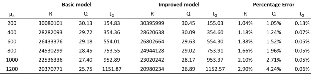
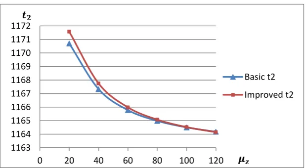
First, we calculate the optimal objective values by varying , the MTTF of given parts. Figure 6 shows that the expected total cost R of both the basic and improved models decreases as increases from 200 to 1200. Also, the values of R in the improved model are always higher than those in the basic model, at a small margin from 1.04% to 2.90%. Figure 7 illustrates that the optimal order quantity Q in both models decreases when increases. Compared with the basic model, the values of Q in the improved model are higher, at a margin from 1.05% to 4.24%. Figure 8 shows that the parts arrival time in both models increases when increases. The values of both are almost identical, verifying that the assertion in Section 2.5 that the two models mainly differ in their handling of Q and R, and, hence the optimal value of is barely affected.

Basic model Improved model Percentage Error

R Q R Q R Q

200 30080101 30.13 154.83 30395999 30.45 155.03 1.04% 1.05% 0.13% 400 28282093 29.72 354.36 28620638 30.09 354.60 1.18% 1.24% 0.07% 600 26433376 29.18 554.01 26802664 29.63 554.30 1.38% 1.52% 0.05% 800 24530299 28.45 753.55 24944128 29.02 753.91 1.66% 1.96% 0.05% 1000 22536336 27.40 952.89 23020242 28.17 953.37 2.10% 2.71% 0.05% 1200 20370771 25.75 1151.87 20980234 26.89 1152.57 2.90% 4.24% 0.06%

(40)

Figure 6. Total cost as increases

Figure 7. Optimal order quantity as increases

Figure 8. Optimal inventory replenishment time as increases

20 22 24 26 28 30 32

0 200 400 600 800 1000 1200

M ill io n s Basic R Improved R 𝝁𝒙 R 25 25.5 26 26.5 27 27.5 28 28.5 29 29.5 30 30.5 31

0 200 400 600 800 1000 1200

Basic Q Improved Q 𝝁𝒙 Q 0 200 400 600 800 1000 1200 1400

0 200 400 600 800 1000 1200

Basic t2

Improved t2

𝝁𝒙

(41)

R Q R Q R Q

20 19042951 26.23 1203.48 19225695 26.60 1203.55 0.95% 1.40% 0.01% 40 19534770 25.93 1188.85 19906533 26.67 1189.13 1.87% 2.76% 0.02% 60 20020055 25.64 1174.12 20587051 26.73 1174.72 2.75% 4.08% 0.05% 80 20498901 25.35 1159.28 21267288 26.78 1160.34 3.61% 5.36% 0.09% 100 20971401 25.06 1144.34 21947276 26.83 1145.97 4.45% 6.62% 0.14% 120 21437640 24.77 1129.3 22627043 26.88 1131.62 5.26% 7.84% 0.21% 140 21897695 24.49 1114.16 23306612 26.92 1117.28 6.05% 9.04% 0.28% 160 22351642 24.21 1098.93 23986003 26.97 1102.95 6.81% 10.23% 0.36% 180 22799548 23.93 1083.61 24665234 27.00 1088.64 7.56% 11.38% 0.46% 200 23241476 23.65 1068.2 25344320 27.04 1074.33 8.30% 12.54% 0.57%

Table 10. Objective values comparison of two models when changes

Next, we consider the impact on the optimal objective value by changing the value of standard deviation ( of the parts lifetime. Figure 9 illustrates that the expected total cost R of both the basic and improved models increases as increases from 20 to 200. This result is natural as a heightened uncertainty level tends to result in more holding and shortage costs. Figure 10 describes an interesting situation that the optimal order quantity Q in the basic model decreases whereas that in the improved model increases when grows. The order quantity Q in the basic model is always higher than in the improved model. The reason might be that failures between and are ignored in the basic model,

(42)

Figure 9. Total cost as 𝒙 increases

Figure 10. Optimal order quantity as 𝒙 increases

Figure 11. Optimal inventory replenishment time as 𝒙 increases

19 20 21 22 23 24 25 26

0 50 100 150 200

M ill io n s Basic R Improved R 𝒙 R 23 24 25 26 27 28

0 50 100 150 200

Basic Q Improved Q 𝒙 Q 1060 1080 1100 1120 1140 1160 1180 1200 1220

0 50 100 150 200

Basic t2

Improved t2

𝒙

(43)

When we increase from 20 to 120, the percentage errors of R, Q , and between the two models decrease.

R Q R Q R Q

20 17476989 20.64 1170.70 18157301 21.95 1171.58 3.75% 5.94% 0.07% 40 27833081 40.51 1167.33 28304380 41.42 1167.75 1.67% 2.19% 0.04% 60 37963663 60.50 1165.78 38263091 61.11 1165.98 0.78% 0.99% 0.02% 80 48092679 80.50 1164.98 48238099 80.84 1165.07 0.30% 0.42% 0.01% 100 58221282 100.50 1164.50 58217152 100.59 1164.52 -0.01% 0.09% 0.00% 120 68349675 120.50 1164.18 68190701 120.34 1164.15 -0.23% -0.14% 0.00%

Figure 12. Total cost as 𝝁 increases

15 20 25 30 35 40 45 50 55 60 65 70

0 20 40 60 80 100 120

M

ill

io

n

s

Basic R

Improved R

𝝁

(44)

Figure 13. Optimal order quantity as 𝝁 increases

Figure 14. Optimal inventory replenishment time as 𝝁 increases

R Q R Q R Q

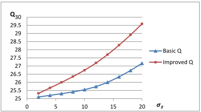
2 14176351 25.10 1164.11 14305746 25.32 1164.32 0.90% 0.87% 0.02% 4 15691930 25.20 1165.65 15948873 25.65 1166.03 1.61% 1.77% 0.03% 6 17206557 25.31 1167.15 17589213 26.00 1167.67 2.18% 2.66% 0.04% 8 18710829 25.41 1168.57 19217067 26.35 1169.20 2.63% 3.57% 0.05% 10 20161980 25.55 1169.75 20787749 26.74 1170.48 3.01% 4.46% 0.06% 12 21521340 25.74 1170.56 22259759 27.19 1171.35 3.32% 5.32% 0.07% 14 22789370 26.01 1171.01 23632083 27.70 1171.86 3.57% 6.12% 0.07% 16 23987166 26.34 1171.20 24925900 28.28 1172.09 3.77% 6.86% 0.08% 18 25137181 26.73 1171.22 26164504 28.91 1172.13 3.93% 7.55% 0.08% 20 26256711 27.17 1171.13 27366204 29.59 1172.07 4.05% 8.18% 0.08%

0 20 40 60 80 100 120 140

0 20 40 60 80 100 120

Basic Q Improved Q 𝝁 Q 1163 1164 1165 1166 1167 1168 1169 1170 1171 1172

0 20 40 60 80 100 120

Basic t2

Improved t2

(45)

14 16 18 20 22 24 26 28

0 5 10 15 20

M ill io n s Basic R Improved R R 25 25.5 26 26.5 27 27.5 28 28.5 29 29.5 30

0 5 10 15 20

Basic Q Improved Q Q 1164 1165 1166 1167 1168 1169 1170 1171 1172 1173

0 5 10 15 20

Basic t2

Improved t2

(46)

In the improved model, we consider when the exact failure happens, which is related to n, the total number of parts for a give PN in the observed fleet. When n increases, R, Q, and increase sharply at the beginning, followed by a flatter slope. The errors of R between the basic and improved models are in the range of 1.79% to 7.83% and the errors of Q between the two models are within 10%. As before, the errors of for the two models remain negligible, lower than 0.15%.

n R Q R Q R Q

100 20161980 25.55 1169.75 20530166 26.38 1170.25 1.79% 3.14% 0.04% 200 20161980 25.55 1169.75 20787749 26.74 1170.48 3.01% 4.46% 0.06% 500 20161980 25.55 1169.75 21041153 27.12 1170.71 4.18% 5.78% 0.08% 1000 20161980 25.55 1169.75 21195563 27.35 1170.86 4.88% 6.58% 0.09% 5000 20161980 25.55 1169.75 21482789 27.79 1171.13 6.15% 8.05% 0.12% 10000 20161980 25.55 1169.75 21585992 27.95 1171.23 6.60% 8.57% 0.13% 100000 20161980 25.55 1169.75 21873606 28.39 1171.51 7.83% 9.99% 0.15%

Table 13. Objective values comparison of two models when n changes

20 20.2 20.4 20.6 20.8 21 21.2 21.4 21.6 21.8 22

0 20000 40000 60000 80000 100000

(47)

2.7 Concluding Remarks

In this chapter, by using the airline industry as the background, we have developed two mathematical models to solve a single PN spare parts inventory management problem, where demands come from installed part failures. We aim to establish an efficient inventory policy that aims to minimize the total cost of stock outs and holding spare parts inventory.

25 25.5 26 26.5 27 27.5 28 28.5 29

0 20000 40000 60000 80000 100000

Basic Q Improved Q Q 1169.6 1169.8 1170 1170.2 1170.4 1170.6 1170.8 1171 1171.2 1171.4 1171.6

0 20000 40000 60000 80000 100000

Basic t2

Improved t2

(48)

(49)

(50)

CHAPTER 3: PROACTIVE SPARE PARTS PROCUREMENT

INVENTORY MANAGEMENT FOR FAILURE-BASED

MAINTENANCE POLICY -

MULTIPLE PART NUMBER (PN) CASE

3.1 Introduction

In this chapter, we study multiple spare parts inventory policies. It is very common that there are multiple spare parts numbers in an inventory system and they face a budget constraint. We aim to establish an efficient spare parts inventory model for multiple PNs to achieve system optimization by considering budget issues and parts delivery time.

(51)

distributions in reliability engineering to predict impending demands. Then we use a multi-product newsvendor model to describe the total expected cost consisting of purchasing, holding, and shortage costs. Unlike the existing newsvendor models that focus on the determination of lot sizes, our proposed models consider the order timing as well. It is apparent that the total cost fluctuates with the lifetime and quantity of installed parts as the uncertainty in their failure influences the duration and numbers of spare parts shortage or overstock. Our proposed nonlinear programming (NLP) models can help spare parts managers to find optimal failure-based procurement inventory policies to minimize cost, with a limited budget constraint.

(52)

3.2 Literature Review

(53)

(54)

2003; Vaughan, 2005). These papers combined age or block replacement with periodic review spare-provisioning policies. Most recently, Wang (2012) presented a joint optimization approach for both the inventory control of the spare parts and the PM inspection interval. Enumeration and stochastic dynamic programming algorithms were used to optimize the order quantity, order intervals and PM intervals. The ordering policy therein is a typical (S, Q) policy in that ordering Q according to inventory level S at the time of ordering under a fixed order interval. To our knowledge, limited research deals with failure-based procurement inventory policies. Also, they typically handle single PN problems. In practice, however, multiple PNs in inventory must be managed from a systematic point of view. In addition decision-makers often have to consider some realistic constraints such as a limited budget.

(55)

In summary, this chapter combine maintenance data and inventory management to deal with a failure-based proactive procurement problem. We use installed parts failure distributions instead of historical demands to predict impending demands. Our inventory model is based on the multi-product newsvendor model which realizes system optimization with a budget constraint. In a single planning period, multiple types of spare parts are considered, and each type of spare parts is identified by a unique PN. Our inventory policy helps a planner to decide how many units to order and when to order to achieve total cost minimization, with a budget constraint. In our research, we assume only one purchase order is placed for each PN in the whole planning horizon. Different PNs can have different order quantities and order times.

3.3 Mathematical Model

3.3.1 Basic Mathematical Model

This research considers a generalized ordering policy for multiple PNs in a single period. For each type of parts i with a given PN, the length of the planning horizon is denoted by

( ) and the order quantity in this period is denoted by . The spare parts for

(56)

density function (·) and cumulative distribution function (·). We also assume (·) and (·) are uncorrelated.

The following notations are used in the model formulation: Indices

= 1, …, m index of parts categories, where m is the total number of parts categories

Parameters

the unit holding cost per unit time of product i the unit shortage cost per unit time of product i planning horizon of product i, can be infinite order lead time of product i

lifetime for each part, a random variable

demand quantity for each PN, a random variable unit price

the budget limitation

the PDF of failure distribution considering lifetime for each part

the PDF of failure distribution considering number of failures for each PN

the CDF of failure distribution considering lifetime for each part

the CDF of failure distribution considering number of failures for each PN

(57)

time point to issue order the parts arrival time

order quantity

The objective is to minimize the expected cost:

Min R = ∑ { ∫ [ ∫ ] ∫

[ ∫

∫

] }

(11)

Budget constraint:

∑

(12)

3.3.2 Improved Mathematical Model

The basic model presented above simplifies the function by assuming MTTF to be the th failure time to determine when the parts shortage period starts. In the improved mathematical model, we consider the exact th failure time to help us determine more accurate order quantity and order time. If we assume is the th failure time for a

given PN i. We also assume that the failure time of PN i is normally distributed, and follows

. is the total number of parts in the observed fleet. Then equation (1)

(58)

∑{ ∫ ( ) ∫

[ ∫

∫

] }

(13) where the failure time is calculated by

( ) ，

(14) with the same budget constraint:

∑

(15)

3.4 Solution Methodology

3.4.1 GAMS and Its Solvers

(59)

3.4.2 A Lagrangian Relaxation Heuristic

Zhang (2010) presented a Lagrangian relaxation heuristic to solve a mixed integer non-linear programming model for the multi-product newsvendor problem with both supplier quantity discounts and a budget constraint. The advantage of this approach is that it can relax the budget constraint and decompose the original problem into a series of sub-problems. It can also provide an error bound between the optimal solution and the approximate solution. Thus, for the improved model, we relax the budget constraint (15) and decompose function (13), then use GAMS and its solvers to solve these decomposed single PN problems.

By introducing a Lagrange multiplier we relax the budget constraint by constructing the following Lagrangian dual problem.

∑

(16) The solution of the above Lagrangian dual problem, , gives the highest lower bound of the solution to the original problem. With a given value of Lagrangian multiplier , the lower bound can be rewritten as follows:

( ) ∑

( )

(60)

∫ ( ) ∫

[ ∫

∫

]

(18)

where the failure time is calculated by

( )

(19) In order to obtain the highest lower bound of the Lagrangian dual problem, a sequence of Lagrangian multipliers are generated to repeatedly calculate the Lagrangian dual. At each iteration, the Lagrangian multiplier is updated by using a bisection method. The complete algorithm is described as follows:

Step 1. Set = 0, =10000 (to be adjusted). Step 2. Let = ( + )/2.

Solve the sub problems with MINOS5. LR = 0; /* Lagrange relaxation value*/ Loop (i,

Solve sub-problem using NLP minimizing R; LR = LR + R).

Step 3: Update Lagrange relaxation value. LR = LR – *K.

(61)

(need to use a scalar to record previous LR) Step 4: Update .

Let ca_gap = ∑ ,

If |ca_gap| < 10E-04 or | - |< 10E-05, Stop.

If ca_gap < 0, then = ; Else = .

Step 5: Go to step 2.

3.4.3 The Combination of the Lagrangian Relaxation Heuristic and Iteration

Method

(62)

In Chapter 2, we noticed that the optimal parts arrival time for the basic and improved models are very close. Thus the iteration method is considered as an effective approach to solve our single PN NLP models. In this section, we continue assuming that all the observed parts failures are normally distributed, that is, for a given PN i, its part lifetime

follows a normal distribution with a mean of and a standard deviation of .

Furthermore, the number of failures for the specified PN ( is normally distributed with a mean of and a standard deviation of . If we assume ∫

, the improved model will be simplified as the basic model. Lagrangian relaxation

Function (8) can be rewritten as

∫ ( ) ∫

[ ∫

∫

]

(20)

There are only two decision variables in function (20), and . The optimal solutioncan be found by the following procedure:

( )[ ] [ ∫

∫ ]

(21)

It follows that

[ ( )] for all

(63)

optimal solution, denoted by *, occurs where

( ) [ ∫ ∫ _] ( ) (22) Also, ∫ [ ] (23)

It follows that

for all

Because the second derivative is nonnegative, the function ( ) is said to be convex.

The optimal solution, say *, occurs where

∫

(24)

{ ( ) [ ( ) ( )] ( ) } (25)

Here is the standard normal density function, and is the standardized

cumulative distribution function for normal density function is the inverse of the cumulative density function for normal density function .

{

[( ) ] [( ) ]

(64)

(26)

Here is the standard normal density function, and is the standardized

cumulative distribution function for normal density function . is the inverse of the cumulative density function for normal density function .

Because the closed forms of and are hard to be determined from function (25) and (26), we develop a numerical algorithm to find solutions. This procedure converges in a finite number of iterations. The steps of the algorithm are

Step 1. Set = 0, = 10000 (to be adjusted). Step 2. Let = ( + )/2.

Step 3. Set , .

Step 4. Use the function (25) to find . Step 5. Use to update by function (26).

Step 6. Update by function (19).

Step 7. If | |< 1.0E-8 the optimal solution is , , and . Otherwise, go to step 4.

Step 8. Calculate by the RHS of function (18).

Step 9. Calculate the Lagrangian relaxation value LR =∑ . Step 10: Update the Lagrangian relaxation value.

LR = LR – *K.

(65)

Y

N

Y

N

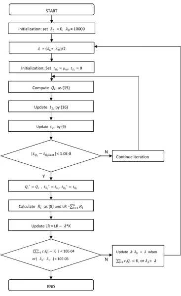
Figure 21. The flowchart of the combination of Lagrangian heuristic and iteration method

Initialization: Set ,

,

Continue iteration

𝜆 = (𝜆𝐿+ 𝜆𝑈)/2 START

Initialization: set 𝜆𝐿 = 0, 𝜆𝑈= 10000

Compute 𝑄𝑖 as (15)

Update 𝑡 _𝑖by (16)

Update 𝑡𝑄𝑖 by (9)

|𝑡𝑄𝑖 𝑡𝑄𝑖𝑙𝑎𝑠𝑡|< 1.0E-8

Calculate 𝑅𝑖 as (8) and LR =∑𝑛𝑖 𝑅𝑖

Update LR = LR – 𝜆*K

Update 𝜆: 𝜆𝑈 = 𝜆 when

∑n 𝑐𝑖𝑄𝑖 , or 𝜆𝐿= 𝜆

END

|∑n

| < 10E-04

(66)

Step 11: Update .

Let ca_gap = ∑ ,

If |ca_gap| < 1.0E-04 or | - |< 1.0E-05, Stop.

If ca_gap < 0, then = ; Else = .

Step 12: Go to step 2.

The flowchart of the algorithm is illustrated in Figure 21.

Once we know and , the optimal time to issue order for a given PN index i can be

found by .

3.5 Numerical Examples and Results

In this section, we give some numerical examples and compare their results for the three methods. As mentioned before, we still assume parts demands follow normal distributions.

(67)

c(i) h (i) s(i) µx(i) days σx(i) days T(i) days µz(i) σz(i) n(i) K

part i=1 449586 307.94 6158.71 243.6 65.9 1825 25 10 200 2.32E+07 part i=2 449586 615.87 2463.48 1218 65.9 1825 25 10 200 2.32E+07

Table 14. Parameter values for two PNs example

The calculation results are summarized in Table 15 for three different methods: GAMS and its solver MINOS 5, the combination of the Lagrangian relaxation heuristic and GAMS /MINOS 5, as well as the combination of Lagrangian relaxation heuristic and iteration method. Compared with single PN examples in Chapter 2, we can see that GAMS/MINOS 5 produces good and accurate results in this small size problem, but it does not work well once it is combined with the Lagrangian relaxation method. However, if the iteration method instead of the GAMS solver is applied to these relaxed and decomposed sub-problems, the optimal solutions are almost the same as GAMS/MINOS 5 results. The tiny difference may be caused by numerical errors. Accordingly, two conclusions can be drawn based on this example: the GAMS/MINOS 5 solver is not reliable once we combine it with the Lagrangian relaxation heuristic due to the complexity of our NLP models. Furthermore, the combination of Lagrangian relaxation heuristic and iteration method is feasible and effective in solving these proposed NLP models.

Q R

GAMS/MINOS5 part i=1 34.53 142.12 181.41 5.64E+07

part i=2 17.00 1,165.46 1,127.56

Lagrangian relaxation &GAMS solver part i=1 0 5121955 1.00E+12 -2.75E+16 part i=2 0 5121955 2.00E+12

Lagrangian relaxation & Iteration part i=1 34.64 140.58 181.55 5.64E+07 part i=2 16.89 1,158.52 1,127.33

(68)

GAMS/MINOS5 Lagrangian relaxation & Iteration

Q R Q R

part i=1 0.02 / 21.60

1.47E+10

139.52 84.27 121.81

8.08E+09

part i=2 155.37 219.96 336.83 169.06 191.14 347.22

part i=3 162.56 109.71 152.65 174.03 101.64 156.08

part i=4 89.54 282.08 556.17 96.41 300.97 573.52

part i=5 29.71 / 231.77 32.41 130.01 238.07

part i=6 66.93 129.79 / 32.41 123.57 220.49

part i=7 339.23 410.73 4.04E+11 182.96 389.90 614.96

part i=8 152.25 427.50 692.77 163.74 425.97 707.14

part i=9 20.27 502.41 673.26 22.46 478.61 689.63

part i=10 183.00 224.27 372.25 198.42 223.82 382.03

Table 16. Calculation results and comparison for the problem with m=10

(69)

the minimum total cost on the right hand side is obviously lower than that on the left. Therefore, the combination of Lagrangian relaxation and iteration has its superiority in solving our proposed multiple PNs NLP models compared with GAMS/MINOS5.

To test the performance and stability of the integrating Lagrangian relaxation and iteration approach in solving large size problems, six instances are randomly generated with the number of PNs (m) ranging from 5 to 2000 with the other parameters such as c(i), h(i), s(i),

, remaining the same in GAMS codes as mentioned in the previous paragraph. The computation results in Table 17 indicate that the integrative Lagrangian relaxation and iteration approach reports extremely good solutions in terms of both solution quality and computing time: the gap between the Lagrangian relaxation value and objective solution value for all the instances are 0. For cases involving up to 200 PNs, the optimal solutions can be found in less than 1 second. Even for large scale cases with thousands of PNs, this approach can obtain results in less than half a minute.

m Bound Solution GAP(%) CPU Times (second)

5 2.90E+09 2.90E+09 0 0.031

10 8.08E+09 8.08E+09 0 0.031

20 1.20E+10 1.20E+10 0 0.062

200 1.24E+11 1.24E+11 0 0.719

1000 7.38E+11 7.38E+11 0 7.063

2000 1.37E+12 1.37E+12 0 21.391

(70)

3.6 Sensitivity Analysis

In order to understand how important parameters affect decision variables, we conduct a sensitivity analysis with the improved multiple PNs model for three different cases, which are typical representations based on our earlier analysis on single PN models in Chapter 2. The basic input parameter values are generated randomly in GAMS and are listed in Table 18. We choose a small size example, m=3, because it is easy to operate and clear to investigate. In each case, we only change one parameter value at a time while the others are kept the same.

c(i) h (i) s(i) µx(i) days σx(i) days T(i) days µz(i) σz(i) n(i) K

part i=1 10387.65 1664.39 38430.80 621.48 104.04 1825 165.56 33.07 367.55

7197117.52 part i=2 50611.68 8019.04 238509.58 1055.44 199.64 1825 45.20 10.50 109.33

part i=3 33067.48 4788.52 103641.02 404.05 119.12 1825 60.18 14.75 150.31

Table 18. Basic values of parameters

K 5997598 6597358 7197118 7796877 8396637 8996397

Q

part i=1 167.715 181.792 195.932 209.967 220.938 220.938

part i=2 44.055 48.959 53.834 58.786 62.989 62.989

part i=3 61.261 67.47 73.704 79.854 84.588 84.588

part i=1 441.573 444.137 447.081 449.874 451.785 451.785 part i=2 686.873 692.081 698.376 704.546 709.016 709.016

part i=3 201.928 205.395 209.23 212.755 215.095 215.095

part i=1 610.056 620.068 630.11 640.158 648.132 648.132

part i=2 1006.393 1029.256 1051.645 1074.337 1093.782 1093.782 part i=3 376.203 388.747 401.172 413.399 422.871 422.871

R SUM 2.72E+09 1.75E+09 1.23E+09 1.02E+09 1.01E+09 1.01E+09

(71)

First, we observe how the budget limit (K) influences our decision variables and objective function value. The test data are summarized in Table 19. K is changed from 5 997 598 to 8 996 397, which is actually from the value of ∑ to 1.5∑ . We can see that Q, , and increase as budget limit K is increased. While the total expected cost R decreases when a higher budget is allowed due to the reduction of shortage cost. The lowest optimal value is obtained at about K=8 396 637 (which is 1.4∑ ), and after that point the decision variables and objective value do not change any more even if the budget limit is further increased. It is due to the reason that the budget limit is likely a binding constraint when K < 8 396 637 and becomes redundant once K ≥ 8 396 637.

(72)

Figure 22. Order quantities change when K increases

Figure 23. Parts arrival times change when K increases

Figure 24. Expected total cost changes when K increases

0 50 100 150 200 250

5990000 6990000 7990000 8990000 9990000 Q(1) Q(2) Q(3) K Q(i) 0 100 200 300 400 500 600 700 800

5990000 6990000 7990000 8990000 9990000

t2(1) t2(2) t2(3) t2(i) K 0.00E+00 5.00E+08 1.00E+09 1.50E+09 2.00E+09 2.50E+09 3.00E+09

5990000 6990000 7990000 8990000 9990000 R

(73)

Next, we investigate how the decision variables and objective function value change as the MTTF ( ) for PN 1 increases. When K=7 197 118 (which is 1.2∑ ), the optimal

replenishment plans for all the three PNs are summarized in Table 20, and are illustrated in Figure 25, 26, and 27. When increases, we can see that the part arrival times for PN 1 are postponed due to their longer expected lifetimes. The part shortage period for PN 1 also starts later due to the same reason, however, the values of and for the other two

parts almost remain at the same levels. Order quantities for the three parts are also kept more or less the same as a result of budget constraint which restricts decision-makers’ purchase of parts. Figure 27 shows that the expected total cost consistently decreases as

increases, which is likely due to the shortage cost savings for PN 1.

312.12 364.14 416.16 468.18 520.2 572.22 621.475

Q

part i=1 198.83 198.398 197.946 197.472 196.975 196.453 195.932 part i=2 53.509 53.558 53.608 53.661 53.717 53.776 53.834 part i=3 73.291 73.353 73.417 73.485 73.555 73.63 73.704 part i=1 138.327 190.258 242.185 294.107 346.024 397.936 447.081 part i=2 697.951 698.015 698.081 698.15 698.223 698.3 698.376 part i=3 208.979 209.016 209.055 209.097 209.14 209.185 209.23 part i=1 322.82 374.532 426.23 477.912 529.578 581.226 630.11 part i=2 1050.157 1050.378 1050.61 1050.853 1051.108 1051.376 1051.645 part i=3 400.351 400.474 400.602 400.736 400.877 401.025 401.172

R SUM 1.28E+09 1.27E+09 1.26E+09 1.25E+09 1.24E+09 1.24E+09 1.23E+09

Proactive and Efficient Spare Parts Inventory Management Policies Considering Reliability Issues

Scholarship at UWindsor

Scholarship at UWindsor

Proactive and Efficient Spare Parts Inventory Management

Proactive and Efficient Spare Parts Inventory Management

Policies Considering Reliability Issues

Policies Considering Reliability Issues

Proactive and Efficient Spare Parts Inventory

Management Policies Considering Reliability Issues

Proactive and Efficient Spare Parts Inventory

Management Policies Considering Reliability Issues

APPROVED BY:

AUTHOR’S DECLARATION OF ORIGINALITY

ABSTRACT

ACKNOWLEDGMENT

TABLE OF CONTENTS

LIST OF FIGURES

LIST OF TABLES

CHAPTER 1: INTRODUCTION

1.1

General Overview

1.2

Proposed Research

1.2.1

Research Topic

1.2.2

Organization of Thesis

CHAPTER 2: EFFICIENT SPARE PARTS INVENTORY

MANAGEMENT FOR AIRCRAFT MAINTENANCE – SINGLE

PART NUMBER (PN) CASE

2.1 Introduction

2.2

Literature Review

2.3

Basic Mathematical Model and Solution Methodology

2.3.1 Basic Mathematical Model

2.3.2 Solution Methodology

2.3.2.1 Numerical and iteration methods

2.3.2.2 Solve the basic model by GAMS

2.4

An Improved Mathematical Model and Solution Methodology

2.5

Numerical Examples and Results

2.6 Sensitivity and Comparative Analyses

2.7 Concluding Remarks

CHAPTER 3: PROACTIVE SPARE PARTS PROCUREMENT

INVENTORY MANAGEMENT FOR FAILURE-BASED

MAINTENANCE POLICY -

MULTIPLE PART NUMBER (PN) CASE

3.1 Introduction

3.2

Literature Review

3.3

Mathematical Model

3.3.1

Basic Mathematical Model

3.3.2

Improved Mathematical Model

3.4

Solution Methodology

3.4.1 GAMS and Its Solvers

3.4.2 A Lagrangian Relaxation Heuristic

3.4.3 The Combination of the Lagrangian Relaxation Heuristic and Iteration

Method

3.5 Numerical Examples and Results

3.6 Sensitivity Analysis