ABSTRACT
JAUNICH, MEGAN KRAMER. Exploring Waste Policy and Management Approaches to Achieve Cost and Environmental Goals: Application of Life-Cycle Optimization Frameworks to Municipal and Electronic Waste Management Case Studies (Under the direction of Dr. Ranji S. Ranjithan and Dr. Joseph F. DeCarolis).
Municipal solid waste (MSW) management is necessary to properly treat and dispose of
the more than 250 million Mg generated each year in the United States. MSW includes ordinary
household waste (e.g., food, packaging), durable goods (e.g., furniture), white goods (e.g., toaster
oven), and electronics (e.g., laptop computer). Worldwide, generation is estimated at over one
billion Mg and could exceed two billion Mg by 2025. Although many safe and effective methods
for waste treatment and disposal exist, each has its own advantages and challenges. Furthermore,
upstream processes, such as waste collection, can influence the effectiveness of downstream
processes, such as recovery of recyclable materials. Additionally, MSW composition is highly
variable and can be directly and indirectly affected by consumer habits, waste management
regulations, and external policies. Because of the interconnected nature and potential effects of
exogenous factors, it is important to holistically assess different waste management options.
The primary goal of solid waste management (SWM) is to protect human health and the
environment. Secondary goals include maximizing resource recovery, including recyclables and
energy, or diverting waste from landfills. Concerns over climate change have made reduction of
greenhouse gas (GHG) emissions a goal as well. SWM activities contribute directly to GHG
emissions, and collection and transportation further contribute to GHG emissions. Such
secondary goals can be achieved through waste management planning and local, regional, or
national policies. For example, many states in the U.S. ban the disposal of yard waste, although
capacity, promoting or supporting composting infrastructure, and reducing landfill GHG
emissions.
Waste management systems at the local, regional, and national scales have been studied
in terms of cost and environmental performance using many different analysis approaches.
However, few have used an integrated optimization modeling framework to analyze real-world
SWM systems with detailed case study data. The goal of this study is to the extend analysis of
hypothetical SWM systems by evaluating how existing or potential waste management policies
influence the cost and environmental performance of real-world systems. Additionally, this study
aims to identify opportunities where a new or different SWM policy may lead to improved
environmental or cost outcomes.
The objectives of this work include: (1) assessing existing electronic and municipal solid
management systems; (2) identifying management alternatives for the present and proposing
options for the future; and (3) using an integrated decision modeling framework to gain insights
into waste management planning. Case study data sets and model representations have been
developed for a municipal SWM system (representing Wake County, North Carolina) and for an
electronic waste management system driven by extended producer responsibility (EPR)
regulations (State of Washington). Results illustrate that existing waste management policies and
practices, sometimes enacted with the intent to achieve environmental and resource conservation
goals, can adversely affect cost and/or environmental performance, while improved outcomes
Exploring the Impacts of Waste Policy and Management Approaches on Cost and Environmental Goals: Application of Life-Cycle Optimization Frameworks to
Electronic and Municipal Solid Waste Case Studies
by
Megan Kramer Jaunich
A dissertation submitted to the Graduate Faculty of North Carolina State University
in partial fulfillment of the requirements for the degree of
Doctor of Philosophy
Civil Engineering
Raleigh, North Carolina 2019
APPROVED BY:
_______________________________ _______________________________
S. Ranji Ranjithan Joseph F. DeCarolis
Committee Co-chair Committee Co-chair
_______________________________ _______________________________
James W. Levis Morton A. Barlaz
ii
DEDICATION
iii
BIOGRAPHY
Megan Kramer Jaunich was born and raised (mostly) in Florida. She graduated Magna
Cum Laude with a Bachelor of Science degree in Mechanical Engineering from Florida Institute
of Technology in 2006, and she continued on to earn a Master of Science in 2007. Following
graduation, she worked as a system safety engineer for Millennium Engineering and Integration
Company at Kennedy Space Center in Florida, during which time she completed a Master of
Engineering degree in System Engineering from Stevens Institute of Technology. In August
2012 she joined the Department of Civil Engineering at North Carolina State University in
Raleigh as a PhD student. Her coursework and research have focused on solid waste
iv
ACKNOWLEDGMENTS
I wish to sincerely thank the members of my committee for their patience, encouragement, and
collaboration during my entire time at NC State; having a kind, supportive, and rigorous group
helped me to persist through times of discouragement and self-doubt. Financial support was so
important to me pursuing and finishing this degree: thanks to various North Carolina State
University funding sources (NCSU Dean's Doctoral Fellowship, Ward Fellowship, College of
Engineering Graduate Merit Award, and the Sustainability Initiative Research Grant from the
Poole College of Management),the Environmental Research and Educational Foundation
(Lonnie C. Poole/Waste Industries Scholarship), and Wake County, North Carolina. I also wish
to acknowledge Hadi Moheb Alizadeh Gashti, who, as part of his Ph.D. studies, led the effort to
develop the mixed integer linear programming model described in Chapter 5. I also want to
thank the many organizations and individuals who provided their time and insights, including
North Carolina State University Surplus Property Services, the Washington Materials
Management & Financing Authority, the Washington State Department of Ecology, Lenovo,
IBM, Wake County Solid Waste Management, the Town of Cary, the Wake County Solid Waste
Technical Advisory Committee, Waste Industries, Global Electric Electronic Processing (GEEP),
v
TABLE OF CONTENTS
TABLE OF CONTENTS ... v
LIST OF TABLES ... viii
LIST OF FIGURES ... xi
Chapter 1. Introduction ... 1
Chapter 2. Solid waste management policy implications on waste process choices and systemwide cost and greenhouse gas performance... 6
Abstract ... 6
2.1 Introduction ... 7
2.2 Modeling Approach ... 9
2.1.1 Functional Unit and System Boundaries... 9
2.1.2 Wake County Waste Characteristics and Waste Generation Sectors ... 11
2.1.3 Scenario Descriptions ... 12
2.1.4 Facility and Process Modeling ... 14
2.3 Results ... 15
2.3.1 Cost-Effective SWM Strategies ... 15
2.3.2 Minimum GHG SWM Strategies... 19
2.3.3 Impact of Separate Collection Requirement ... 19
2.3.4 Results Summary ... 21
2.4 Sensitivity ... 22
2.5 Policy Implications ... 25
Chapter 3. Exploring alternative solid waste management strategies for achieving policy goals ... 30
Abstract ... 30
3.1 Introduction ... 31
3.2 Modeling Approach ... 33
3.2.1 Model Description ... 33
3.2.2 Case Study and Data Description ... 34
3.2.3 Wake County Scenarios ... 36
3.2.4 Method for Generating Alternative Optimal Solutions ... 37
3.2.5 Scenario Refinement based on SWM Personnel Feedback ... 39
3.3 Results ... 39
3.3.1 Comparisons of Alternative SWM Strategies with Bounding Cases... 40
3.3.2 Mass Flows and Waste Collection Schemes of SWM Alternatives ... 42
3.3.3 Feedback from Wake County SWM Experts ... 45
3.3.4 Revised Strategies and Results Summary ... 48
3.4 Policy Implications ... 49
Chapter 4. Life-cycle modeling framework for electronic waste recovery and recycling processes ... 53
Abstract ... 53
4.1 Introduction ... 54
vi
4.2.1 E-waste Characterization ... 60
4.2.2 E-waste Recovery and Recycling Processes ... 60
4.3 Washington Case Study ... 69
4.3.1 Washington State Case Study Description ... 70
4.3.2 Ranking Process Model Input Parameters by Relative Impact on Output Coefficients ... 72
4.3.3 Variability of Input Parameters at E-waste Processing Facilities and Comparison with Empirical Data ... 74
4.3.4 Alternative E-waste Management Scenarios ... 77
4.4 Results: Comparison of Alternative E-waste Management Scenarios ... 77
4.5 Discussion ... 80
Chapter 5. Life-Cycle Optimization Framework for Integrated Electronic Waste Management Considering Cost and Environmental Impacts ... 83
Abstract ... 83
5.1 Introduction ... 84
5.2 Modeling Approach ... 87
5.2.1 Cost Objective Function: E-waste Recovery and Recycling ... 91
5.2.2 Emissions Objective Function: E-waste Recovery and Recycling ... 93
5.2.3 Constraints ... 94
5.3 Illustrative Example of an E-waste Take-back System ... 97
5.4 Illustrative Results ... 99
5.4.1 Impact of Drop-off Facility Convenience: User versus System Optimal Scenario... 99
5.4.2 Limited Capacity and Different E-waste Product Mix ... 103
5.4.3 Illustrative Sensitivity ... 110
5.5 Discussion ... 111
5.6 Acknowledgements ... 113
Chapter 6. Concluding Remarks and Future Work ... 114
References 116 APPENDICES ... 133
Appendix A. Supporting Information for Chapter 2 ... 134
A.1 Background Information ... 134
A.2 Waste Composition ... 137
A.3 Default Waste Composition ... 140
A.4 Alternate Waste Composition ... 156
A.5 Model Parameters ... 159
A.5.1 Collection ... 165
A.5.2 Material Recovery Facilities ... 170
A.5.3 Composting ... 173
A.5.4 Anaerobic Digestion ... 173
A.5.5 Mass Burn Waste-to-Energy Combustion (WTE) ... 174
A.5.6 Transportation ... 175
vii
A.5.8 Electricity Grid... 176
A.6 Supplemental Results and Discussion ... 177
A.7 Results Summary Data ... 180
Appendix B. Supporting Information for Chapter 3 ... 182
B.1 Modeling to Generate Alternatives Formulation ... 182
B.2 Bounding Case Results ... 182
B.3 Additional Results ... 183
Appendix C. Supporting Information for Chapter 4 ... 188
C.1 E-waste Modeling Framework ... 188
C.1.1 Notations ... 188
C.1.2 Additional Modeling Framework Details ... 190
C.1.3 E-waste recycling facility process model ... 190
C.1.4 Electricity and Intermediate Economic Calculations ... 191
C.2 Recovered Material Default Properties ... 194
C.3 Washington case study input parameters values ... 195
C.3.1 Costs and emissions from personal vehicles attributable to electronic waste recycling ... 197
C.4 Supplemental Results ... 204
viii
LIST OF TABLES
Table 2-1. Description of model scenarios. ... 13
Table 2-2. Mitigation cost for cost-minimized cases in relation to Base_Case cost ($/MTCO2e). ... 18
Table 3-1. Description of model scenarios. ... 37
Table 3-2. Collection Scheme Difference Metrics for the All Scenario. ... 45
Table 3-3. Revised strategies based on feedback from WCSWM. ... 49
Table 4-1. Process-level parameters varied: Parameter distributions for Monte Carlo analysis to estimate system total cost, revenue, emissions, and emissions offsets. ... 78
Table 4-2. Distribution Mean for Product Mix Systems and Routing Scenarios: Unit Cost and Emissions. ... 80
Table 5-1. Decision Variables and Indices for the Mixed-Integer Linear Programming Model. ... 88
Table 5-2. Population, generation, and product mix for two different e-waste streams: Baseline and Alternative Product Mix. ... 98
Table 5-3. Distances between residence areas h, drop-of facilities d, e-waste recycling facilities p, and material treatment facilities s. ... 98
Table 5-4. Percent difference in costs and emissions between system optimal value and user optimal value for Product Mix Scenarios (PM1 and PM2) with capacity constrained for e-waste recycler 1. ... 104
Table 5-5. Drop-off facility used by and distance from residence area for system optimal and user optimal cases (all product mix and capacity scenarios). ... 104
Table A-1. Integrated Solid Waste Management Case Studies. Studies include at least two SWM processes and considers system-level implications; the “X” shows which processes were included. ... 135
Table A-2. Population and Number of Households Serviced for Each Sector. ... 138
Table A-3. Adaptation of Wake County Data About Waste Composition to SWOLF Waste Fractions. ... 141
ix Table A-5. Composition of Residual Waste by Sector: Single-family, Multi-family, and
Convenience Centers ... 146
Table A-6. Composition of Source-Separated Recyclables by Sector (%) ... 149
Table A-7. Composition of Source-Separated Organics by Sector (%) ... 151
Table A-8. Collection Separation Efficiencies (%). Quantity of Waste Item Collected for Recycling Divided by Total Generation of Waste Item (Single-family (SF) Municipalities, Multi-family (MF), and Convenience Center (CC)) ... 152
Table A-9. Average Waste Composition by Sector: Single-family (SF) Municipalities, Multi-family (MF), and Convenience Center (CC). ... 154
Table A-10. Alternate Waste Composition by Sector: Single-family (SF) Municipalities, Multi-family (MF), and Convenience Center (CC) ... 157
Table A-11. Abbreviations for Wake County Waste Generating Sectors and Facilities ... 159
Table A-12. Existing and Potential Future SWM Facilities: Location, Current Capacity, Minimum Build and Expansion Capacities, and Minimum Percent of Built Capacity Which Must be Utilized ... 160
Table A-13. The Initial Build Cost Coefficient and the Expansion Cost Coefficient for Each Capacity Process ... 160
Table A-14. The Utilization Cost Coefficient Associated with Each Process and Waste Item ($/Mg) ... 161
Table A-15. GHG Emission Coefficient Associated with Each Process and Waste Item (kg CO2e/Mg). Negative Values Indicate Net GHG Offsets for the Specified Waste Fraction at the Specified Treatment Process ... 163
Table A-16. Default Input Values for Collection Process Model ... 166
Table A-17. Sector-specific Collection Process Model Inputs ... 169
Table A-18. Collection Route-to-Facility (Drf) and Facility-to-Garage (Dfg) Distances ... 170
Table A-19. Mixed Waste and Single-stream MRF Separation Efficiency and Utilization Cost Parameters ... 172
Table A-20. Selected Input Parameters for Future WTE Facility ... 174
x Table A-22. Electricity Grid Power Generating Mix for Default and Alternate Cases ... 177
Table A-23. Net GHG (MTCO2e) Comparison by Process: +MW (max diversion) and
+WTE (70% and Max Diversion) ... 178
Table A-24. Sample Results Table (Table S24) from Results workbook “Supplemental
Info Summary Results Tables S25-S128.xlsx” ... 181
Table B-1. Material recovery for recycling with single stream recycling in Base case compared with recovery of recyclable material from mixed waste using a
mixed waste MRF (e.g., Scenario R2) ... 186
Table B-2. Summary results: collection, annualized cost, GHG, and diversion... 187
Table C-1. Key Processing Activities of an E-waste Management System; their
interactions among the processes are shown in Figure 4-1 ... 190
Table C-2. Default costs for materials managed at e-waste recycling facility. Revenue from recovered materials is indicated as a positive value ($/kg) and cost for disposal of residual waste is indicated as a negative value. Residual is
assumed to be landfilled... 194
Table C-3. E-waste generation, product mix, and device re-sale associated with the
Washington state “E-cycle” program (2013) ... 195
Table C-4. Washington E-cycle program: e-waste weight and composition
characteristics ... 196
Table C-5. Dedicated fraction values used for four categories of convenience ... 198
Table C-6. Default input parameter value and percentage change in net cost ($/kg) and CO2 (kg CO2/kg) at drop-off facility based on 20% increase in individual
parameter values ... 199
Table C-7. Default input parameter value and percentage change in change in net cost ($/kg) and CO2 (kg CO2/kg) at e-waste recycling facility based on 20%
increase in individual parameter values ... 200
Table C-8. Net cost and emissions for e-waste management facilities as estimated by model simulation with Washington case study data compared with reported Washington E-cycle program costs ... 204
Table D-1. Input parameters for illustrative analyses ... 205
xi
LIST OF FIGURES
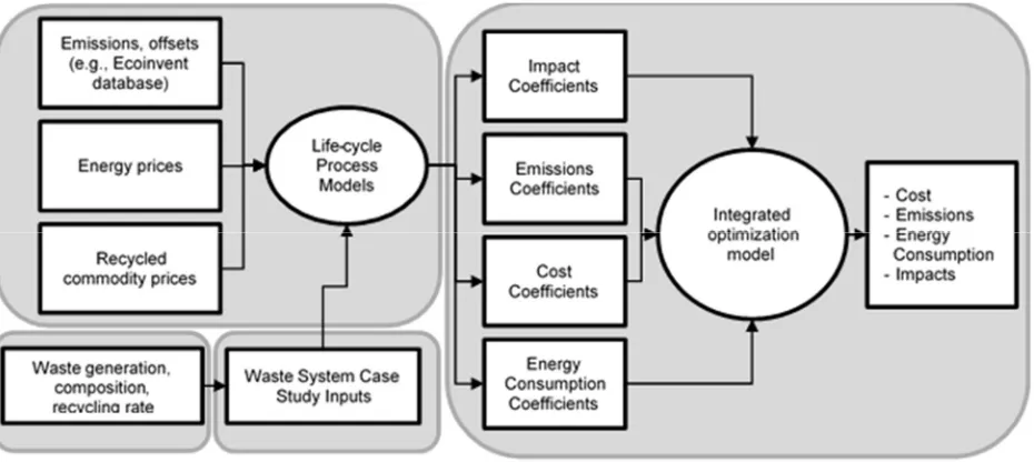
Figure 1-1. Integrated Modeling Framework: Life-cycle process model interaction with data sources and optimization model. ...4
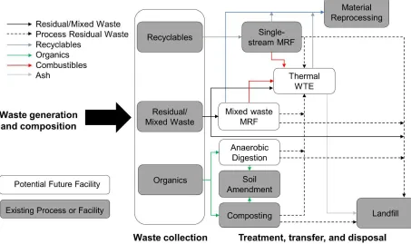
Figure 2-1. Potential mass flows through the prevailing and future SWM system for Wake County, North Carolina. Residual waste includes MSW that remains after source-separated recyclables and organics (only yard waste included in current system) are collected. Mixed waste collection can be used to collect all generated waste. Aluminum and ferrous metal in WTE bottom ash can be separated and recycled, but remaining bottom ash and fly ash are assumed to not be beneficially used in this study. Waste generation and composition are presented in Appendix A.2 and facility details in Appendix A.3. Adapted
from (Levis et al., 2014). ...11
Figure 2-2. Cost, GHG emissions, facility utilization, and mitigation cost for Base_Case and Food Waste (+FW+AD) scenarios. The sum of “% of Total Waste” may exceed 100% since MSW may be managed at more than one facility. AD was selected by the model only when the objective is minimizing GHG
emissions. ...16
Figure 2-3. Cost, GHG emissions, facility utilization, and mitigation cost at different diversion levels for scenarios (a) Base_Case, (b) +MW, (c) +WTE, and (d) +MW+WTE. Total waste percentage may exceed 100% since MSW may be managed at more than one facility. Separate collection of single-stream recyclables and yard waste are required. Alternate facility utilization increases to meet the minimum cost objective as the diversion target
increases. ...17
Figure 2-4. Cost, GHG emissions, facility utilization, and mitigation cost for +MW+WTE+AnyCollection scenarios at increasing budget constraints. Mixed waste MRF and WTE use increased as the diversion constraint was increased while minimizing cost. At the minimum GHG, mixed waste MRF is used for material recovery prior to sending residual to WTE for energy
recovery. ...20
Figure 2-5. Net annualized cost, landfill diversion, and waste treatment choices for Base_Case, +MW+WTE (required separate collection), and
xii energy recovery provides GHG emissions reductions at a moderate cost
increase. The fraction of each slice of a particular pie chart is representative of the fraction of generated waste entering each indicated treatment process in the respective solution. ...22
Figure 3-1. Potential mass flows through the current and future SWM system for Wake County, North Carolina. Residual waste includes MSW that remains after source-separated recyclables and organics are collected. Mixed waste collection can be used to collect all generated waste. Aluminum and ferrous metal in WTE bottom ash can be separated and recycled but remaining bottom ash and fly ash are assumed to have no beneficial use in this study.
(Jaunich et al., 2019) ...35
Figure 3-2. Net annualized cost, landfill diversion, and GHG emissions offsets for scenarios a) All, b) AD, c) No MWMRF, d) No WTE, and e) comparing all alternative solutions to the current system with all treatment processes enabled but requiring separate collection of recyclables and yard waste (Bounding: Separate Collection) and the current system with all treatment and collection processes enabled (Bounding: Any Collection) at various diversion levels. The center of each circle indicates the cost and diversion value. Cost and GHG offsets (larger circle means higher offsets) tend to increase with increased diversion for scenarios with the same collection scheme. Cost, GHG, and diversion are presented in Table B-2. Panel e) displays linear regression for Separate Collection (Base 28% diversion through max diversion at 82%) and Any Collection (min cost 7% diversion through 70% diversion). The boxed area represents the solution space explored (> 35% diversion, > min cost, > min GHG, < cost in Base. Several SWM alternatives overlap in panels a-e. Mass flows for results are described in Appendix B.2. ...41
Figure 3-3. Base Wake County Scenario: Cost, GHG emissions, and landfill diversion for the current Wake County SWM system. Total residential waste
generation for the county (approximately 401,000 Mg) is shown initiating from single family (SF), multi-family (MF), and convenience center (CC) sectors. Waste flows are approximately to scale. Mass flow quantities are
presented in Table A-24. ...43
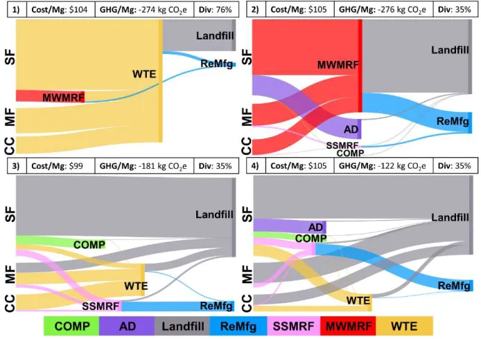
Figure 3-4. All Scenario: Cost, GHG emissions, and landfill diversion for four strategies (panels 1-4) identified through MGA for the scenario that includes all SWM treatment processes. Total residential waste generation for the county (approximately 401,000 Mg) is shown initiating from single family (SF), multi-family (MF), and convenience center (CC) sectors. Waste flows are
xiii Figure 3-5. No WTE Scenario: Cost, GHG emissions, and landfill diversion for four
strategies (panels 1-4) identified through MGA for the scenario that includes all SWM treatment processes except WTE is excluded. Total residential waste generation for the county (approximately 401,000 Mg) is shown initiating from single family (SF), multi-family (MF), and convenience
center (CC) sectors. Waste flows are approximately to scale...44
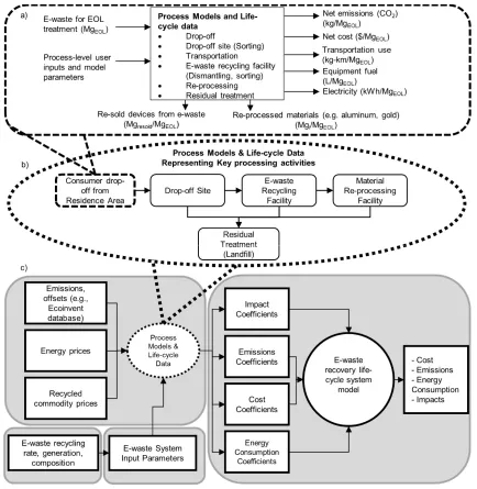
Figure 4-1. The integrated e-waste management system modeling framework. A generic e-waste management process is shown in (a) and details are described in Appendix Table A1. Process models include incoming e-waste product mix and composition and process input parameters and computes the output coefficients (net emissions and cost) for that process. The functional unit is the total quantity of e-waste, defined by the amount and material
composition of each product type, going to EOL treatment per year. (b) E-waste originates in residences, is transported to a drop-off site, sorted, and is prepared for shipment to a recycling facility. Materials recovered at the recycling facility are sent for reprocessing into recycled materials, and residual is sent to residual treatment (landfill). (c) The process models interface with data sources and the integrated e-waste recovery model, which allows the modeling framework to capture the changes in costs and emissions at both the process and the system level as (e.g., due to
composition changes of an electronic product). ...59
Figure 4-2. Costs, emissions, and mass flows for e-waste management processes. Costs are incurred for aggregating e-waste at a drop-of site, processing at a recycling facility, and disposing of residual waste. Revenues are earned from the sale of functional devices and from the sale of recovered materials for production of recycled materials/re-processing. Costs are incurred for transportation with each waste flow to a facility and are allocated to the drop-off or inter-facility transportation processes. Emissions are the result of electricity and fossil fuel use at a drop-of site or e-waste recycling facility. Process emissions occur from the production of recycled materials/re-processing. Emissions offsets are the result of avoided production of new devices and virgin materials. Transportation emissions occur with each waste flow to a facility and are allocated to the drop-off or inter-facility
transportation processes. ...68
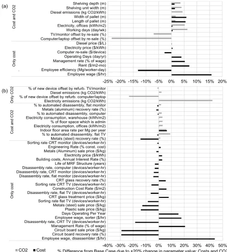
Figure 4-3. Percent change from base case output values (emissions and cost) based on 20% increase in input parameter value associated with the process model. Changes less than 0.1% not shown. Results are grouped by impact on process model cost and/or CO2 coefficients then ranked based on magnitude
xiv workday (more shifts meant more electricity consumption), electricity grid
emissions, and offsets from device re-sale had the largest impact on CO2.
For recycling facility (b), disassembly rate (worker efficiency) and recovery and sale price of circuit boards had the largest impact on cost, while offsets from device re-sale, the assumed CO2 intensity of electricity, and the portion
of devices being treated with automated equipment had the largest impact
on CO2...73
Figure 4-4. Net emissions and net cost per kg at drop-off site (kg CO2/kg and $/kg).
Monte Carlo simulation distribution, model-estimated net value based on
default input data, and Washington E-cycle program cost estimate. ...75
Figure 4-5. Contribution by process to cost, revenue, emissions, and offsets for System 1 (the base case) with half of e-waste routed to a manual recycler and half to a more automated recycler (Scenario 1). The Drop-off of e-waste is the major contributor to cost and CO2 emissions. Revenue from recovered
materials is attributed to the recycling facility in this framework, but
emissions offsets are attributed to material re-processing. ...79
Figure 5-1. E-waste recovery system that represents the flow of e-waste items and materials from generation in residence areas to eventual material remanufacture or disposal, via drop-off collection sites and recycling
facilities. ...89
Figure 5-2. Life-cycle process model: summary of inputs and outputs. ...89
Figure 5-3. Impact of Variation in Dedicated Fraction df on User Cost and System Cost. ...100
Figure 5-4. Contribution of User Cost (Residence Area h to Drop-off Facility d, RA-DO) to Transportation Cost for System (S) and User (U) Optimal Cases (% and $). ...102
Figure 5-5. Contribution of each process to cost/revenues and emissions/offsets. ...106
Figure 5-6. Mitigation Cost for Product Mix and Capacity Scenarios. ...109
Figure 5-7. Sensitivity of System Net Cost and Emissions to Input Parameters, Net Cost and Net Emissions Minimization. ...111
xv waste and recyclables. One convenience center sector accepting all waste
generated by all sites is modeled. Many composting facilities exist and are not shown in this figure; composting facilities are modeled as a single
facility. ...136
Figure A-2. Total Mass of Waste Generated (1000 Mg), and the Split of Recyclables, Yard Waste, and Residual Waste for each Residential Sector. Food waste is generally not separately collected in Wake County and is thus included with residual waste in this figure. ...139
Figure A-3. Cost, GHG Emissions, Facility Utilization, and Mitigation Cost for
+MW+WTE at Increasing Budget Constraints. Budget levels were selected at even increments between the net system costs in the least cost and least GHG solutions, with additional budget levels between the first and second budget levels to mirror the additional diversion levels between 30 and 40% shown in main body Figure 3 (b)-(d). Separate collection of single-stream recyclables and yard waste was required, mixed waste MRF and WTE were enabled. Mixed waste MRF and WTE use increased to meet minimum GHG objective as the budget constraint was loosened. GHG emissions are
minimum at the maximum budget constraint. At that level, mixed waste MRF is used for material recovery prior to sending residual to WTE for
energy recovery...179
Figure A-4. Cost, Landfill Diversion, GHG Emissions, and Mitigation Cost for +MW+WTE and +MW+WTE+AnyCollection. Requiring separate waste collection (+MW+WTE) results in higher system net cost than when separate collection is not required (+MW+WTE+AnyCollection). Annualized cost and mitigation cost tend to increase with increasing diversion, but mitigation cost savings compared to the base case can be achieved for a wide range of diversion levels when separate collection is not required. ...180
Figure B-1. Scenario 2. AD: Annualized cost, GHG emissions, and landfill diversion for the Wake County SWM system with mixed waste MRF and WTE enabled, and AD required for separately-collected organics (food and yard waste). Total residential waste generation for the county (approximately 401,000 Mg) is shown initiating from single family (SF), multi-family (MF), and
convenience center (CC) sectors. Waste flows are approximately to scale. ...183
xvi (SF), multi-family (MF), and convenience center (CC) sectors. Waste flows
are approximately to scale. ...184
1
Chapter 1. Introduction
Globally, more than 1 billion metric tons (Mg) of municipal solid waste (MSW) is
generated annually (Hoornweg and Bhada-Tata, 2012), as well as an estimated 50 million Mg of
electronic waste (e-waste). In the U.S., consumer electronics comprise approximately 2% of
MSW, while e-waste, as a whole, approaches closer to 5% (i.e., including appliances, batteries,
and electronics). Waste generation continues to grow worldwide, and its proper management is
essential to protect human health, minimize impact on the environment, and promote effective
use of material and energy resources. While material and energy recovery technologies have the
potential to reduce the cost and environmental impacts associated with waste management,
efficient collection, transportation, treatment, and disposal choices are essential to ensure the
most cost-effective and environmentally beneficial waste management system.
Waste management policies, legislation, and management choices influence, and
sometime dictate, the way waste is collected, treated, and disposed. While material recycling and
landfill diversion are two common management approaches intended for achieving favorable
environmental and material recovery outcomes, it is not clear that such policies necessarily and
consistently minimize environmental, economic or related impacts. For instance, the European
Union has set landfill diversion targets and requires pre-treatment for biodegradable waste prior
to disposal in a landfill; however, when landfills have effective gas collection with energy
recovery, organic waste disposal in a landfill may have lower net GHG emissions than
composting, depending on the assumed soil amendment offset (Hodge et al., 2016). Banning
yard waste from landfill is common and is understood by the public to be generally beneficial to
the environment. In typical U.S. practice, most yard waste is composted and most food waste
2 compared with several anaerobic digestion alternatives—high solids, co-digestion with industrial
waste or sewer sludge (Yoshida et al., 2012).
In the context of electronic waste (e-waste), a constituent of MSW, recycling has been
promoted in the U.S. and globally through Extended Producer Responsibility (EPR) legislation.
Such legislation holds manufacturers responsible for the recovery and recycling of their
products; however, a recent study by Esenduran and Kemahlioglu-Ziya (2015) suggested that
actions taken by companies in response to EPR legislation might increase the total environmental
impact of certain products. For example, a manufacturer electing to comply with EPR legislation
via its own e-waste recovery program instead of through a collective program made up of
multiple manufacturers may reduce the overall collection rate for a particular region, thereby
potentially reducing the efficiency of the collective program and consequently increasing its cost
and/or emissions. Additionally, recent declines in the demand for recyclable materials have
raised concerns about the destination of source-separated recyclables and whether the costs
outweigh the benefits (Corkery, 2019). These examples illustrate a potential disconnect between
policies intended (at least in part) to have favorable environmental implications and the real
outcomes of their implementations in waste management practices.
E-waste and MSW management systems are complex, involving many processes,
existing infrastructure, and stakeholders. Economic and environmental tradeoffs among different
solid waste management (SWM) systems are not easily generalized and are heavily dependent on
the waste system characteristics that are location-specific (De Feo et al., 2016; Ripa et al., 2017).
A systematic approach is needed to analyze integrated SWM strategies while simultaneously
considering local waste characteristics, waste management infrastructure, and competing
3 potential success at achieving stated environmental or policy goals and to support SWM policy
development and implementation. A life-cycle-based approach is useful for holistically
evaluating the system-wide cost and environmental implications of SWM decisions, while an
optimization-based approach further enables systematic exploration and identification of
efficient solutions. Previous work has proposed various life-cycle and optimization modeling
frameworks for analyzing SWM systems, although only a few have applied such frameworks to
case studies. This dissertation research expands on prior studies by implementing detailed,
real-world, case study data in life-cycle optimization frameworks with the objective of exploring the
impacts of existing and future waste management approaches and policies on cost and the
environment. Furthermore, this dissertation methodically identifies alternative effective
strategies to achieve competing goals by meeting modeled objectives while enabling the
consideration of the strategies’ performance with respect to unmodeled objectives.
Two case studies were developed based on existing waste management systems: (1)
Wake County, North Carolina’s municipal SWM system for managing residential MSW, and (2)
the state of Washington’s electronics EPR program which is funded by original equipment
manufacturers (OEM). These case studies incorporate recent waste generation characteristics,
existing infrastructure, and geographic details to provide a realistic representation of the waste
management systems. The goal of this research is to study these systems using an appropriate
integrated life-cycle modeling framework to answer the following questions: (1) What impact do
waste management policies or approaches have on cost and environmental performance of waste
management systems? and (2) What are potential opportunities for improvements through the
4 The life-cycle frameworks connect process-level life-cycle models with an integrated
optimization model and enable in-depth analysis of waste management systems. Life-cycle
assessment (LCA) is a tool used to systematically evaluate environmental impacts and costs of
products or services through all stages of their life cycle, and to compare performance of
different systems that provide the same function or service. Figure 1-1 shows the general
modeling framework which connects data sources with life-cycle process models that provide
cost, emissions, energy consumption, and impact coefficients to the optimization model;
Chapters 2 and 5 have model- and system-specific schematics for the Wake County MSW and
Washington e-waste analyses, respectively.
Figure 1-1. Integrated Modeling Framework: Life-cycle process model interaction with data sources and optimization model.
Chapters 2 through 5 were written as individual research papers (Appendices A-D
provide background information and correspond with Chapters 2-5, respectively). Chapters 2 and
3 focus on MSW and Chapters 4 and 5 focus on a single category of MSW, e-waste. Chapter 2
discusses methodological details of developing a data set to represent the large, real-world SWM
5 context of Wake County’s management goals, existing SWM constraints, and future
considerations. Chapter 3 further explores the solution space to identify maximally different
strategies that meet cost and environmental goals and can further be considered by decision
makers in terms of unmodeled objectives such as practicality of implementation, public
perceptions, or management preferences. Chapter 4 discusses methodological details of
developing a data set to represent the large, real-world e-waste management system of the U.S.
state of Washington in a life-cycle framework. The framework is used to estimate quantitatively
the contribution of e-waste management processes to cost and greenhouse gas emissions, and to
compare alternative systems representing possible management choices. Chapter 5 builds upon
the life-cycle approach in Chapter 4 to investigate a mathematical programming model for
optimizing the e-waste management system considering cost and select environmental impacts
for a simplified version of the Washington case study. A discussion of the influence of waste
management policies and approaches on the performance of waste management systems is
included in Chapter 6.
Overall this dissertation aims to evaluate how municipal waste and e-waste management
approaches and policies affect cost and environmental performance of waste management
systems. Identifying opportunities for waste management system improvement in terms of cost,
GHG emissions reductions, and/or landfill diversion, while quantifying associated adverse
effects on those parameters will help inform and aid decision makers. Given the large and
complex nature of waste management, it is imperative to holistically represent site-specific waste
management systems in an integrated framework to systematically assess and compare waste
management alternatives to support policy and management goals while considering cost,
6
Chapter 2. Solid waste management policy implications on waste process choices and systemwide cost and greenhouse gas performance
Abstract
Solid waste management (SWM) is a key function of local government and is critical to
protecting human health and the environment. Development of effective SWM strategies should
consider comprehensive SWM process choices and policy implications on system-level cost and
environmental performance. This analysis evaluated cost and select environmental implications
of SWM policies for Wake County, North Carolina using a life-cycle approach. A
county-specific data set and scenarios were developed to evaluate alternatives for residential municipal
SWM, which included combinations of a mixed waste material recovery facility (MRF),
anaerobic digestion, and waste-to-energy combustion in addition to existing SWM infrastructure
(composting, landfilling, single stream recycling). Multiple landfill diversion and budget levels
were considered for each scenario. At maximum diversion, the greenhouse gas (GHG) mitigation
costs ranged from 30 to 900 $/MTCO2e; the lower values were when a mixed waste MRF was
used, and the higher values when anaerobic digestion was used. Utilization of the mixed waste
MRF was sensitive to the efficiency of material separation and operating cost. Maintaining the
current separate collection scheme limited the potential for cost and GHG reductions.
Municipalities seeking to cost-effectively increase landfill diversion while reducing GHGs
7
2.1 Introduction
Proper solid waste management (SWM) is important to protect human and environmental
health and is a critical function of local government. At the local level, waste collection may
comprise as much as 40% of municipal solid waste (MSW) management budgets (Chalkias and
Lasaridi, 2009) and may be the most fossil fuel-intensive process in SWM systems (NREL,
1995). Landfills, which nationally receive over 50% of municipal solid waste, are estimated to be
the third largest contributor to anthropogenic methane (CH4) emissions in the U.S. (17.6%), and
landfilling, composting, and waste incineration are reported to be responsible for approximately
2% of U.S. greenhouse gas (GHG) emissions (U.S. EPA, 2017). Many local and state policies
have been enacted with the goal of improving the cost or environmental performance of SWM
systems. For example, yard waste bans have been enacted to increase landfill diversion (NERC,
2017) and some communities (e.g., Portland, OR; San Francisco, CA; Seattle, WA) have
mandated food waste diversion for residential and/or commercial generators (Portland City
Code, 2012a; Portland City Code, 2012b; San Francisco City Ordinance, 2009; Seattle Municipal
Code, 2015). Because the economic and environmental tradeoffs among different SWM system
designs are location-dependent (Ripa et al., 2017; De Feo et al., 2016) and influenced by existing
or potential SWM practices and policies (Laurent et al., 2014), strategies enacted with the intent
of accomplishing environmental goals may not necessarily achieve them universally (e.g., the
benefits of recycling will vary based on the availability of reprocessors and materials markets).
Furthermore, piecemeal policies targeted for a specific waste flow or process may have
unintended consequences elsewhere in the system that could potentially undermine the intended
purpose of the policy. Thus, systematic integrated analysis of SWM alternatives in consideration
8 is necessary to evaluate whether proposed SWM strategies achieve the intended goals and to
support development of appropriate policies and plans for future SWM.
Interest in the impact of existing municipal SWM practices on environmental
performance, cost, and other metrics is illustrated by regional and national SWM case studies.
Appendix Table A-1 presents studies that included two or more solid waste processes. In some
cases, a life-cycle methodology was used to compare baseline scenarios with alternative SWM
approaches (Jia et al., 2018; Yadav and Samadder, 2018; Noya et al., 2018; Stanisavljevic et al.,
2018; Aleisa and Al-Jarallah, 2018; Starostina et al., 2018; Hadzic et al., 2018; Ripa et al., 2017;
Liu et al., 2017; Marino et al., 2017; Syeda et al., 2017; Bjelic et al., 2017; Grzesik, 2017; De
Feo et al., 2016; Yay, 2015; Fernandez-Nava et al., 2014; Song et al., 2013; Belboom et al.,
2013; Thanh and Matsui, 2013; Nouri et al., 2014), while other studies employed different
methods, such as waste flow analysis (Tunesi et al., 2016) or multi-period mixed integer linear
programming (MILP) along with life-cycle data to analyze geographically different regions (e.g.,
optimizing for cost by maximizing profit (Tan et al., 2014), maximizing profit while assigning a
financial cost to environmental impacts (Harijani et al., 2017). Notably, the number of systematic
case studies in the context of U.S. SWM systems is small, even though comprehensive integrated
analyses (e.g., life-cycle-based case studies such as Kaplan et al., 2009) in the U.S. context could
contribute to decision support as municipalities increasingly seek SWM strategies to achieve cost
and environmental goals while addressing landfill diversion challenges (Levis et al., 2014).
The objective of this study is to assess the cost, environmental performance (i.e., net
GHG emissions), and landfill diversion potential for Wake County, North Carolina (NC),
considering current and prospective alternative SWM strategies from a life-cycle perspective,
9 choices. Wake County is a large, suburban county in the center of North Carolina which operates
its own landfill (South Wake) with approximately 25 years of remaining capacity (Wake County,
2018). County management has a goal to maximize the life of the South Wake Landfill while
simultaneously considering cost and environmental impacts. Additional objectives of this paper
are to: (1) provide methodological insights on modeling a complex SWM system using real data
and a life-cycle optimization decision-support tool (the Solid Waste Life-cycle Optimization
Framework, SWOLF) (Levis et al., 2013); and (2) perform policy-relevant optimization analyses
to support SWM decision-making. The prospective SWM options included combinations of the
following: addition of anaerobic digestion (AD), thermal treatment by mass-burn
waste-to-energy (WTE), and a mixed waste material recovery facility (MRF), as well as changes to the
current collection practice.
2.2 Modeling Approach
This section describes how the Wake County SWM system was represented in SWOLF.
More generally, the methodological steps described here provide a roadmap for other researchers
to develop thorough, data-driven representations of their own case studies.
2.1.1 Functional Unit and System Boundaries
A life-cycle approach was used to quantify GHG emissions, costs, and landfill diversion
associated with current and potential SWM strategies for Wake County. The functional unit is
the annual mass of residential mixed MSW ready for end-of-life treatment (e.g., set out at the
curb), and reference flows are the masses of individual waste items (e.g., brown glass, aluminum
cans), as detailed in Section 2 of the SI. Landfill diversion is defined as the fraction of generated
waste that does not go to a landfill (e.g., landfilled bottom ash from waste-to-energy does not
10 collected independently, with the remaining waste referred to as residuals. Collected waste is
managed at existing or prospective future SWM facilities (Figure 2-1). The system boundary
includes final disposal of residual waste in a landfill and the reprocessing of recovered recyclable
materials including beneficial offsets from avoided primary energy and material production.
SWM options considered were based on existing practice in Wake County and other available
technologies in a U.S. context. The analysis used a 100-year time horizon for environmental
emissions. One-hundred-year global warming potential (GWP) was calculated using values from
the Intergovernmental Panel on Climate Change (IPCC) Fifth Assessment Report which reported
that one kg CH4 is equivalent to 34 kg CO2 over 100 years (IPCC, 2013). The Wake County
SWM system was modeled and implemented using SWOLF, which uses a multistage
optimization approach based on a mixed-binary linear program, to identify efficient SWM
11
Figure 2-1. Potential mass flows through the prevailing and future SWM system for Wake County, North Carolina. Residual waste includes MSW that remains after source-separated recyclables and organics (only yard waste included in current system) are collected. Mixed waste collection can be used to collect all generated waste. Aluminum and ferrous metal in WTE bottom ash can be separated and recycled, but remaining bottom ash and fly ash are assumed to not be beneficially used in this study. Waste generation and composition are presented in Appendix A.2 and facility details in Appendix A.3. Adapted from (Levis et al., 2014).
2.1.2 Wake County Waste Characteristics and Waste Generation Sectors
Wake County had a population of approximately 1.02 million in 2015 and was the fastest
growing metropolitan area in the U.S. between 2000 and 2010 (U.S. Census Bureau, 2010).
Wake County residential waste was assumed to originate from one of three sectors: (1)
single-family residential, (2) multi-single-family residential, or (3) drop-off convenience centers. The county
consists of 12 incorporated cities and towns that collect or have contracts for the separate
collection of yard waste, recyclables, and residual waste from single-family residences. Waste
collection from multi-family units are modeled as two sectors: one representing Raleigh since
12 Each city or town operates convenience (i.e., drop off) centers to collect recyclables and residual
waste from residents, and the county operates centers for residents of unincorporated areas. All
convenience centers are modeled as a single sector. Table A-4presents the mass generated by
each residential sector and the amount initially diverted from landfill disposal (i.e., collected for
yard waste composting or recycling). Table A-5 through A-7 present the composition of each
separately collected waste stream for each sector and the source-separated fraction (i.e., the
collection separation efficiency) for each waste item for each sector.
The management of commercial waste was not included in this study since commercial
waste is not collected or managed by the municipalities and counties in North Carolina. As some
commercial waste is nonetheless managed by the county’s landfill, potential implications of
commercial waste management are discussed with the results.
2.1.3 Scenario Descriptions
Scenarios were created to represent current practice and plausible SWM alternative
strategies (i.e., technology choices and mass flows) that align with the county’s management
goals. These scenarios include the addition of food waste collection, AD, WTE, and a mixed
waste MRF (Table 2-1). For each scenario, SWOLF was used to identify SWM strategies that
meet specified objectives (e.g., minimize cost, maximize landfill diversion, minimize GHG
emissions) subject to waste management targets and constraints.
In the scenario representing current practice in Wake County (Base_Case), recyclables
and yard waste are collected separately. For the least-cost strategies, different combinations of
processes are enabled, and the minimum cost solutions were found at incrementally increasing
diversion requirements. For the least-GHG strategies, minimum GHG solutions were found at
13
Table 2-1. Description of model scenarios.
Scenario Name Description Model Objective(s)
[Key Constraints]
Base_Case
Current practice involves separate collection of residential recyclables to a single-stream MRF and yard waste to composting facilities (single-family residences only)
Cost
+FW+AD
Base_Case plus food waste co-collected with yard waste and AD enabled (but not required to be selected). Diversion is fixed based on assumed source separation rates.
Cost, GHG
+MW Base_Case with mixed waste MRF enabled Cost [Diversion]
+WTE Base_Case with WTE enabled Cost [Diversion]
+MW+WTE Base_Case with mixed waste MRF and WTE both enabled Cost [Diversion] GHG [Cost]
+MW+WTE+AnyCollection As in +MW+WTE, but separate collection of recyclables and yard waste is not required
Cost [Diversion] GHG [Cost]
The county is considering food waste diversion, and some small-scale food waste
diversion efforts are already in place (primarily drop-off). In addition to the current practice in
Wake County, +FW+AD enables food waste collection and AD. Similarly, additional MSW
treatment technologies (i.e., mixed waste MRF and WTE) are also enabled, independently and
simultaneously, to identify alternative SWM strategies that could increase landfill diversion
(scenarios +MW, +WTE, and +MW+WTE) while still potentially utilizing the existing separate
(yard waste, single-stream recyclables and residual) waste collection system. As SWM goals
could be achieved through alternative strategies that need not necessarily include separate
collection of recyclables or yard waste, +MW+WTE+AnyCollection is included to represent the
least constrained situation in which any facility type and any collection scheme could be used in
14
2.1.4 Facility and Process Modeling
SWOLF embeds life-cycle process models that compute waste-item-specific unit cost and
emissions coefficients for individual processes in the SWM system, including waste
collection(Jaunich et al., 2016), transfer stations (simplified version of (Pressley et al., 2015)),
landfills (Levis and Barlaz, 2011), composting (Levis and Barlaz, 2011), AD (Levis and Barlaz,
2011), MRFs (Pressley et al., 2015), mass burn WTE (updated version of Harrison et al., 2000),
and material reprocessing (U.S. EPA, 2001). A collection model was created for each sector
using collection activity data from multiple sources (Wake County, 2012; Wake County, 2018;
SCS Engineers, 2011; NC Department of Environmental Quality, 2017). The landfill model
reflects South Wake Landfill operations. Composting facilities in Wake County use windrows
and the resulting compost is assumed to be land applied with appropriate mineral fertilizer
production offsets (Levis and Barlaz, 2011). Digestate from a potential new AD facility is
assumed to be aerobically cured after AD and prior to land application. The single-stream MRF
model represents a facility similar to those used in Wake County. The model representing a
potential future mixed waste MRF facility uses lower recovery rates than the single-stream MRF
facility to account for lower separation efficiency and losses due to higher contamination
expected at mixed waste facilities as described in (Pressley et al., 2015) (Table A-19). The
potential future WTE facility is assumed to be state-of-the art with landfilling of residual ash
after iron and aluminum recovery. Each process has associated capital and operating costs (Table
A-13 and A-14), as well as GHG emissions coefficients (Table A-15) and user-specified
minimum build and expansion capacities (Table A-12). The life-cycle models used for each
15 Utilization of existing Wake County facilities (South Wake landfill, composting sites,
single-stream MRFs) incurs no initial build cost, while building new facilities (WTE, AD, mixed
waste MRF) does. Other than sector- and site-specific facility details, waste characteristics, and
waste collection parameters, the default SWOLF data and process models were used (Levis et
al., 2013). The default electricity grid mix was assumed to be that of the Southeast Electric
Reliability Corporation (SERC), which includes North Carolina (Table A-22).
2.3 Results
2.3.1 Cost-Effective SWM Strategies
Food waste collection was enabled (+FW+AD) to increase diversion compared to
Base_Case (Figure 2-2) by increasing food waste source-separation to 50% from 0% in
Base_Case and enabling its collection with the current yard waste stream. When cost is
optimized for +FW+AD, food waste is treated with single-family yard waste at a composting
facility, which reduces GHG by 5.9 kg CO2e/Mg waste, increases cost by 0.47 $/Mg, and
increases diversion from 28% to 31%. When GHG emissions are optimized, food and yard waste
are sent to AD to achieve the same 31% diversion; however, this reduces GHG emissions by 6.6
kg CO2e/Mg waste. Since food waste is 70-80% moisture (Lopez et al. 2016; Hodge et al.,
2016), its rapid decomposition and volume reduction would result in less than 1% effective
savings in landfill volume (De la Cruz and Barlaz, 2010).
The mitigation cost is used to estimate the cost-effectiveness of an alternate scenario for
reducing GHG emissions compared to Base_Case; it is calculated by dividing the increase in cost
by the decrease in emissions. The U.S. Environmental Protection Agency’s (EPA) social cost of
carbon provides context for the calculated mitigation costs. The social cost of carbon is the dollar
16 emitted in a given year. The EPA’s 2020 estimate for the social cost of carbon is 46 $/MTCO2e
(r = 3%) with the baseline assumption of severity and 136 $/MTCO2e at high severity (U.S.
EPA, 2017).
The +FW+AD cost increases primarily due to additional processing costs for composting
or using AD; GHG emission savings are due to reductions in net GHG at the landfill, and GHG
offsets from electricity production at AD (Figure 2-2). The mitigation cost for the cost-optimized
+FW+AD solution is 98 $/MTCO2e and 839 $/MTCO2e when GHG is optimized (Table 2-2).
Thus, food waste diversion with composting yields a small increase in landfill diversion and
GHG benefits, while the same diversion by using AD would cost more and provide greater GHG
reductions.
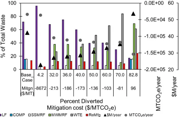
Figure 2-2. Cost, GHG emissions, facility utilization, and mitigation cost for Base_Case and Food Waste (+FW+AD) scenarios. The sum of “% of Total Waste” may exceed 100% since MSW may be managed at more than one facility. AD was selected by the model only when the objective is minimizing GHG emissions.
Solutions at several diversion levels for Base_Case, +MW, +WTE, and +MW+WTE
(Figure 2-3) help illustrate the effect of adding different SWM technologies on diversion, energy
recovery, or recovery of materials that are not separated by the waste generator (at rates
17 Base_Case, the annualized cost increases to $45M for +MW with a mitigation cost of 30
$/MTCO2e. The maximum diversion achievable by processing all residual waste at the mixed
waste MRF prior to landfilling is nearly 39% compared to 28% for Base_Case. WTE use can
achieve 80% diversion since waste is reduced to ash and metal is recovered from the bottom ash;
however, net GHG emissions offsets are higher for +MW at maximum diversion (39%) than that
for +WTE at all diversion levels except at the maximum diversion (i.e., all residual waste is
incinerated). Up to 70% diversion, emissions offsets from WTE electricity generation do not
outweigh the increase in net emissions resulting from reduced material recovery, reduction in
carbon storage at the landfill, and additional emissions from the combustion of plastics (Table
A-23).
At every diversion level, mitigation cost for +WTE is lower than that for GHG-optimized
+FW+AD, but it is higher than that for +MW (Table 2-2); this is primarily because the capital
Figure 2-3. Cost, GHG emissions, facility utilization, and mitigation cost at different diversion levels for scenarios (a) Base_Case, (b) +MW, (c) +WTE, and (d) +MW+WTE.
Total waste percentage may exceed 100% since MSW may be managed at more than one facility. Separate collection of single-stream recyclables and yard waste are required. Alternate facility utilization increases to meet the minimum cost objective as the diversion target
18 cost of WTE is between that of AD and of a mixed waste MRF. Thus, while WTE can be used to
achieve higher diversion and lower net GHG emissions, a mixed waste MRF can achieve
moderate GHG reductions at a lower cost.
The Wake County system achieves the best diversion and GHG emissions when both a
mixed waste MRF and WTE are included (+MW+WTE). At 32% diversion, only a mixed waste
MRF and landfill are used for residual waste (identical to +MW). The assumed minimum build
capacity of WTE (48,000 Mg/yr) is sufficient to achieve 36% diversion cost-effectively without
a mixed waste MRF. Use of only a mixed waste MRF achieves no more than 40% diversion;
addition of WTE is needed to attain 40% or higher diversion, and the combined use of WTE and
mixed waste MRF is more cost effective than using WTE alone. At the maximum diversion, all
collected MSW is initially treated at a mixed waste MRF prior to incineration at WTE.
Mitigation costs at different diversion targets for +MW+WTE lie between those for +MW and
+WTE (Table 2-2).
Table 2-2. Mitigation cost for cost-minimized cases in relation to Base_Case cost ($/MTCO2e). Diversion Constraint
Scenario 30% 31% 32% 34% 36% 38% 39% 40% 50% 60% 70% >80%b
+FW+AD
(least cost) N/A 98a - - - -
+FW+AD
(least GHG) N/A 839a - - - -
+MW 14 17 18 23 27 34 34a - - - - -
+WTE 96 96 96 96 96 96 99 101 110 108 112 131a
+MW+WTE 14 17 18 23 96 96 64 54 62 72 85 96a
a Max diversion level
b For +WTE, maximum diversion is 80%. For +MW+WTE, maximum diversion is 83%.
19
2.3.2 Minimum GHG SWM Strategies
To investigate cost-effective SWM strategies to reduce GHG emissions, GHG
emissions-minimizing strategies were identified at increasing budget levels, starting with Base_Case cost
and then increasing incrementally to the cost of the least GHG strategy (Figure A-3). Mixed
waste MRF and WTE were enabled as in +MW+WTE; also, separate collection of yard waste
and recyclables was imposed. Thus, the recyclables separated by households for single stream
recyclables collection are directed to the single stream MRF and yard waste to composting. The
GHG emissions minimizing strategies use the mixed waste MRF to increase recovery of
recyclable materials not separated by residents and consequently increase the associated GHG
offsets from material reprocessing. As the budget increases incrementally, the use of WTE (with
ash going to landfill) instead of the landfill increases to treat the mixed waste MRF residual.
Thus, the GHG optimizing strategies vary in terms of diversion and mitigation cost (Figure A-3).
2.3.3 Impact of Separate Collection Requirement
The optimal cost and optimal GHG strategies indicate that the collection process is a
major contributor to cost and GHG emissions, and that the contribution is higher when separate
collection is required. Taking the sum of the absolute value of all SWM processing costs and
GHG emissions (i.e., the total magnitude of processing costs and GHG emissions including net
revenue and offsets), waste collection contributes 84% to costs and 30% to GHG emissions in
Base_Case. Using the 50% diversion case as an example, collection contributed 80% to the sum
of the absolute value of process costs and 17% to GHG emissions when separate collection is
required (+MW+WTE). Because the contribution of collection to cost and GHG emissions is
large, and since compliance with material landfill bans and other policies could be achieved
20 waste and/or recyclables, an additional scenario (+MW+WTE+AnyCollection) was considered
(Table 2-1) where all collection and treatment processes in +MW+WTE were enabled (but not
required).
Compared to Base_Case, the cost-effective +MW+WTE+AnyCollection strategies have
lower cost and GHG emissions for all diversion levels analyzed up to 70% (Figure A-4). With no
separate recycling collection requirement, fewer materials go to a single-stream MRF. Instead, to
increase diversion more cost-effectively, a mixed waste MRF is utilized at lower diversion levels
and WTE is utilized between 40% and 70% diversion (Figure 2-4). To achieve the maximum
diversion (82.5%), all residual waste is sent to a mixed waste MRF, with MRF residual going to
WTE, and landfill is used for WTE ash only; also, costlier options of separate yard waste
collection and composting are used to divert yard waste. Collection costs for
+MW+WTE+AnyCollection strategies at all diversion levels are approximately half those of
Base_Case, except at maximum diversion when the same collection scheme as Base_Case is
Figure 2-4. Cost, GHG emissions, facility utilization, and mitigation cost for
21 used, resulting in 3.5 times more GHG emissions offsets and over 82% diversion (compared to
28% in Base_Case) at 27% greater cost (mitigation cost is 96 $/MTCO2e).
The GHG emissions minimizing strategy for +MW+WTE+AnyCollection cost
approximately 11% more than the Base_Case (mitigation cost is 31 $/MTCO2e) and has 4.5
times more GHG emissions offsets with over 78% diversion. Each strategy for
+MW+WTE+AnyCollection costs 28% to 36% less and has 1% to 66% higher GHG emissions
offsets than +MW+WTE strategies at the same diversion targets. Thus, alternate treatment
options (+MW+WTE) increase opportunities for GHG emissions reductions but at added cost;
however, when coupled with no separate collection requirement (+MW+WTE+AnyCollection),
both cost savings and GHG emissions reductions improve.
2.3.4 Results Summary
Net system GHG emissions tend to decrease with increasing diversion, but not
monotonically. If landfill diversion is the primary goal, both diversion and environmental goals
(i.e., net GHG emissions reductions) could be met at a lower cost by not requiring separate
collection of yard waste, recyclables, and residual waste. For example, if GHG reduction is the
primary goal while not exceeding 125% of the current cost, a combination of WTE and mixed
waste MRF could be used to achieve 60% diversion and more than four times the GHG offsets of
Base_Case (Figure 2-5). But, at the same cost, 80% diversion could be achieved with more than
22
Figure 2-5. Net annualized cost, landfill diversion, and waste treatment choices for Base_Case, +MW+WTE (required separate collection), and +MW+WTE+AnyCollection (any collection scheme). Cost and GHG offsets tend to increase with increased diversion for scenarios with the same collection scheme. Within a given diversion range (e.g., 40-45%), there is a large
difference in cost and net GHG offsets. The primary driver of the cost difference is the collection scheme used. In general, a combination of mixed waste MRF with material recovery for
remanufacturing and WTE with energy recovery provides GHG emissions reductions at a
moderate cost increase. The fraction of each slice of a particular pie chart is representative of the fraction of generated waste entering each indicated treatment process in the respective solution.
2.4 Sensitivity
Several +MW+WTE strategies were analyzed to evaluate the sensitivity of the results to
select process model parameters. We explored the impact on results due to changing the default
settings for the energy grid, mixed waste MRF efficiency parameters (material recovery
efficiency and processing costs), and the assumed waste composition.
The default electricity grid was changed to two alternative grids: “Coal” consisted
entirely of coal-generated electricity, while “Natural Gas” consisted of the national average split
of natural gas generating technologies (i.e., 33% combined cycle, 50% combustion turbine, 17%
steam) (Table A-22). The set of treatment processes selected and the mass flows to meet the
23 assumption has a large impact on the calculated net GHG emissions and associated mitigation
costs. For all model runs where GHG savings are realized with increased net cost (i.e., positive
mitigation costs), the mitigation cost ranges from 6 to 53 $/MTCO2e when using the “Coal” grid,
and 31 to 399 $/MTCO2e for the “Natural Gas” grid. Thus, if the grid were to shift towards more
natural gas than coal (i.e., less GHG-intensive), the price of GHG mitigation would increase and
could exceed the 2017 U.S. EPA estimate (136 $/MTCO2e, assuming high severity impacts) for
the social cost of carbon, since a cleaner grid reduces the emission offsets from waste-based
energy or recovered resources.
Mixed waste MRF appears in all GHG- and cost-optimized strategies for +MW+WTE.
To explore the sensitivity to mixed waste MRF performance, the material separation efficiency at
the MRF was decreased by 10% and the processing cost was increased by 10% (Table A-19);
consequently, none of the cost-optimized solutions utilizes a mixed waste MRF, suggesting that
the cost-effectiveness of using a mixed waste MRF instead of WTE to achieve higher diversion
is sensitive to the MRF’s efficiency. This also indicates that the effectiveness of the mixed waste
MRF in improving the sustainability of the solid waste system is sensitive to incoming and
outgoing rates of contamination and how they affect separation efficiencies, revenues, and
beneficial offsets. When the separation efficiencies and processing costs were changed by 5%,
use of mixed waste MRF is reduced at each diversion level (e.g., at 70% diversion, when
efficiency is reduced by 5%, mixed waste MRF utilization is approximately 10% of that for the
default efficiency). However, for GHG-optimized solutions, a mixed waste MRF is used to the
same extent as in the default runs even with a 40% decrease in separation efficiency. The
mitigation costs at each budget level are within 20% of the default runs, ranging from 54 to 123
24 the recovered materials were reduced due to contamination in the outgoing streams. Applying the
reduced mixed waste MRF efficiency parameters to +MW+WTE+AnyCollection produced
similar results; mixed waste MRF is not used in cost-optimized scenarios but is used to the same
level in the GHG-optimized solutions as in +MW+WTE+AnyCollection.
Sensitivity to waste characteristics was examined by considering an alternative waste
composition that was developed based on the annual change in the per capita generation of each
waste material estimated by extrapolating the annual percentage change in U.S. per capita MSW
generation from 2000 to 2010 (U.S. EPA, 2012) to 2045 (Table A-10). Recyclable glass
generation decreases by over 2% per year during that period, PET container generation increases
by 3%, and all types of recyclable paper decrease by 1 to 5% per year. The total change in per
capita generation for each material through 2045 was limited to ±25%. The 2045 composition, as
a plausible future waste composition, was then applied to the default waste generation amount.
Use of SWM treatment processes is largely insensitive to the change in composition, and
variations in net cost at each intermediate diversion constraint are within ~7% of default. The
total amount of separately collected waste is lower in the alternate composition scenario since
there is less yard waste and recyclables, which also reduces the collection costs. In the maximum
diversion case, the mass of material recycled or composted is reduced by 33%, but total
diversion is reduced only by 0.1% since residual waste is still combusted. The minimum GHG
emissions are 3% higher than that for the default setting, primarily due to fewer offsets from
WTE, composting, landfill, and remanufacturing due to reduction in the generation of recyclable