Effects of Variable Prey and Cohort Dynamics on Growth of
Young-of-the-Year Estuarine Bluefish: Evidence for Interactions
between Spring- and Summer-Spawned Cohorts
FREDERICK
S. SCHARF*
Department of Biology and Marine Biology, University of North Carolina at Wilmington, Wilmington, North Carolina 28403, USA
JEFFREY
A. BUCKEL
Department of Zoology, Center for Marine Sciences and Technology, North Carolina State University, 303 College Circle, Morehead City, North Carolina 28557, USA
KENNETH
A. ROSE
Department of Oceanography and Coastal Sciences and Coastal Fisheries Institute, Louisiana State University, Baton Rouge, Louisiana 70803, USA
FRANCIS
JUANES
Department of Natural Resources Conservation, University of Massachusetts, Amherst, Massachusetts 01003, USA
JAMES
H. COWAN, JR.
Department of Oceanography and Coastal Sciences and Coastal Fisheries Institute, Louisiana State University, Baton Rouge, Louisiana 70803, USA
Abstract.—Previous field studies of bluefishPomatomus saltatrixhave documented variation in young-of-the-year (age-0) growth rates among years and between spring- and summer-spawned cohorts. However, the potential factors responsible for generating variable growth in age-0 bluefish have not been investigated. We constructed an individual-based model that combined size-dependent bluefish foraging with a bioenergetics model to quantify the potential effects of variable prey fish dynamics on first-summer growth of juvenile bluefish. We used long-term monitoring data to define baseline conditions and calibrate the model. We then performed three simulation experiments designed to assess the effects of initial density and arrival timing of prey species and bluefish cohorts on bluefish length distributions on October 1. Simulation experiments indicated that spring-spawned bluefish were robust to fluctuations in prey dynamics because of a spawning strategy that ensures temporal overlap with a diversity of prey fish species. In contrast, summer-spawned bluefish were sensitive to variation in prey fish dynamics because of their dependence on a single prey species. Model results also revealed the potential for the time of arrival and the initial density of the spring-spawned cohort to affect the growth of the summer-spring-spawned cohort. Our findings demonstrate that population-level interactions between bluefish and their prey can be complex and have a considerable influence on the early growth rates of the summer-spawned cohort.
Bluefish Pomatomus saltatrix have a worldwide subtropical distribution and support commercial and recreational fisheries throughout their range (Juanes et al. 1996). Adult landings and juvenile recruitment indices provide evidence of a declining bluefish population along the U.S. East Coast during the past two decades (Mid-Atlantic Fishery Management Council 1998; Munch and Conover 2000), and historical records indicate large interannual fluctuations
in abundance (Baird 1873). Recent efforts to identify potential causes of interannual variation in bluefish abundance have focused on the relationship between the survival of larval and juvenile life stages and the eventual recruitment success of annual cohorts (Con-over et al. 2003).
The life history of bluefish in the western Atlantic Ocean has been described in detail elsewhere (Juanes and Conover 1995; Hare and Cowen 1996; Juanes et al. 1996). Briefly, adults spawn in offshore waters over the continental shelf of the U.S. East Coast, egg and larval stages develop in shelf waters, and juveniles recruit to nearshore oceanic and estuarine habitats. Two pulses of juvenile recruits arrive in mid-Atlantic estuaries each
* Corresponding author: [email protected] Received March 4, 2005; accepted March 12, 2006 Published online September 7, 2006
1266
summer (Nyman and Conover 1988; McBride and Conover 1991), representing survivors from spring and summer spawning events identified from otolith-derived birth dates. Upon entry into estuaries, juvenile bluefish become piscivorous and exhibit an increase in their growth rate. This increase in growth rate is due, in part, to the switch from invertebrate prey to piscine prey (Juanes and Conover 1994). After spending the summer in mid-Atlantic estuaries, bluefish migrate southward in autumn and overwinter in the South Atlantic Bight (Buckel et al. 1999b; Munch and Conover 2000).
Factors that influence the advection and mortality of egg and larval stages have been proposed as important to bluefish recruitment success (Hare and Cowen 1993, 1996, 1997; Munch and Conover 2000). However, little is known about how year-class success is shaped by processes affecting growth and survival of young-of-the-year (hereafter, age-0) bluefish during their residency in estuaries. Considerable interannual varia-tion in juvenile growth rate and body size attained before fall migration has been documented for both the spring- and summer-spawned cohorts (McBride and Conover 1991; McBride et al. 1995; Munch and Conover 2000). Higher bluefish cohort loss rates, implying higher mortality, were observed by McBride et al. (1995) during years of slow growth rates. Slower growth could be caused by density-dependent compe-tition among bluefish for their prey. Growth rate variability in the early juvenile period can have important consequences for the survival and recruit-ment of marine fishes (Campana 1996; Sogard 1997). Moreover, the effects of variable growth and body size in bluefish may not be limited to their estuarine period; slow estuarine growth could interact with size-de-pendent mortality due to predation or energetic limitations during the southward migration and over-wintering to further influence year-class success (Shuter and Post 1990).
Growth rate variability in fishes is often difficult to explain because multiple environmental (e.g., water temperature) and biological (e.g., prey availability) factors can be important and are often confounded. The availability of appropriately sized prey can be affected by several processes and may have a large effect on bluefish growth trajectories during their first summer. By initiating spawning at southern latitudes, the spring-spawned bluefish cohort is spring-spawned in advance of many other fish species that occupy mid-Atlantic estuaries during the summer (Juanes et al. 1994; Juanes and Conover 1995). These later-spawning fish species then become prey for the spring-spawned bluefish cohort (Juanes et al. 1993; Juanes and Conover 1995; Buckel and Conover 1997; Buckel et al. 1999a).
The summer-spawned bluefish cohort, however, is spawned at more northern latitudes and does not recruit to estuarine waters until midsummer. Later estuarine arrival limits the diet of the summer-spawned bluefish cohort to a much smaller subset of fish prey than that experienced by the spring-spawned cohort; diets of summer-spawned bluefish are dominated by bay anchovy Anchoa mitchilli in both estuarine (Juanes and Conover 1995; Buckel 1997) and oceanic waters (Buckel et al. 1999b). By affecting predator–prey size relationships and encounter probabilities, variation in prey dynamics from year to year (e.g., timing of spawning, density, growth rate) may alter the timing and degree of piscivory in bluefish, which can in turn affect bluefish growth (Juanes and Conover 1994; Buckel et al. 1998). Furthermore, because bluefish diets differ between spring- and summer-spawned cohorts, the influence of prey fluctuations may be cohort specific.
Individual-based models are ideally suited to examine size-dependent interactions (e.g., predator– prey relationships) among individual organisms and have been successfully used to evaluate the effects of these interactions on fish populations (Adams and DeAngelis 1987; Rice et al. 1993). Recent studies have combined individual-based foraging models with bio-energetics models to explore the potential effects of multiple interacting factors on fish feeding, growth, and size-dependent recruitment success (Dong and DeAn-gelis 1998; Mason et al. 1998; Burke and Rice 2002). Here, we report the results of simulations using an individual-based model that couples size-dependent foraging with a bioenergetics model to evaluate the potential consequences to age-0 bluefish growth of variation in the dynamics of prey fish populations. The model was constructed with the use of established bioenergetics relationships (Steinberg 1994; Hartman and Brandt 1995) and size-dependent foraging relation-ships (Scharf et al. 2003). We used the model to quantify the potential effects of variation in the population dynamics of summertime estuarine prey fishes on the body sizes achieved by spring- and summer-spawned bluefish just before their southward migration in early fall. Specifically, we present the results of three simulation experiments designed to evaluate the effects of variation in (1) the timing of prey fish appearance, (2) prey fish density, and (3) bluefish cohort density and estuarine arrival timing.
Methods
Model Description
age-0 bluefish during their summer and early-fall residency in mid-Atlantic estuarine systems. Aspects of the ecology of juvenile bluefish have been studied throughout much of the species’ U.S. East Coast range, and several common features emerge. The first feature is the summer appearance in inshore waters of at least two distinct juvenile cohorts that have been demonstrated to represent the survivors from spring and summer spawning events (Kendall and Walford 1979). Al-though the mechanism producing two juvenile cohorts (e.g., distinct spawning periods or differential transport success) has yet to be precisely determined (Hare and Cowen 1993), the inshore appearance of two pulses of age-0 bluefish is ubiquitous. The presence of spring-and summer-spawned bluefish cohorts is evident in nearly all years of the National Marine Fisheries Service’s fall bottom trawl survey conducted between Cape Hatteras, North Carolina, and the Gulf of Maine (Munch and Conover 2000). Two distinct age-0 cohorts have been observed in every state between Maine and North Carolina, where extensive studies of juveniles exist (McBride and Conover 1991; Creaser and Perkins 1994; McBride et al. 1995; Able et al. 2003).
Two other features general to mid-Atlantic bluefish are their dependence on piscine prey and their rapid growth during their first summer. The small, schooling species within the families Atherinidae, Clupeidae, and Engraulidae are prevalent in age-0 bluefish diets (Juanes et al. 1993; Juanes and Conover 1995; Buckel et al. 1999b; Scharf et al. 2004). Furthermore, bluefish selection for fish prey is passively size dependent, as evidenced by the strong negative size dependence of prey fish capture success (Scharf et al. 2003). Consumption of mainly fish prey by age-0 bluefish promotes very rapid growth during their first summer (Juanes and Conover 1994); individual bluefish often realize four- to fivefold increases in length between the time of estuarine arrival and southern migration in fall. Mean estimated growth rates in several mid-Atlantic systems generally exceed 1 mm/d and have approached 2 mm/d (McBride and Conover 1991; McBride et al. 1995; Able et al. 2003). Growth rates of age-0 bluefish in the mid-Atlantic also demonstrate appreciable levels of variation both among years and among individuals within years (McBride and Conover 1991; McBride et al. 1995; Able et al. 2003). Factors influencing variable growth of age-0 bluefish and the interaction of spring-and summer-spawned cohorts have not been thorough-ly investigated.
Our model attempts to capture these general features of juvenile bluefish ecology, and the simulations that we outline below are designed to explore processes that may influence the growth and sizes achieved by spring-and summer-spawned age-0 bluefish before their
southerly fall migration. We configured the model and designed the exploratory simulations using exten-sive empirical data collected in the lower Hudson River estuary, one of several large estuarine nursery areas for age-0 bluefish in the mid-Atlantic. Although we used Hudson River data, our model is not designed to generate predictions of bluefish dynamics for specific years or conditions in the Hudson River; rather, we used Hudson River data to ground-truth our model so we would have more confidence in its general predictions. By means of system-specific adjustments to environmental inputs and prey fish community composition and dynamics, the model can be adapted to explore similar hypotheses in other estuarine and nearshore oceanic systems where age-0 bluefish have been studied. The relative success of the spring- and summer-spawned bluefish cohorts has been the subject of much recent interest (Conover et al. 2003). Our model was constructed as a general exploratory framework within which we could begin to identify potential factors affecting the processes of feeding and growth of age-0 bluefish that may eventually contribute to cohort recruitment success.
Model overview.—Model simulations begin on calendar day 100 (April 9), continue through calendar day 274 (October 1), and follow the daily growth and mortality of individual spring- and summer-spawned bluefish in a single, well-mixed, 5,000-m3spatial box. The initial appearance of bluefish in the baseline model occurs on calendar day 169 (June 18). The environment in the spatial box is defined by daily water temperature and the densities and size distributions of multiple cohorts of four prey fish species: bay anchovy, striped bass Morone saxatilis, river herring Alosa spp., and Atlantic silversidesMenidia menidia. Individual blue-fish from each of the spring- and summer-spawned cohorts are introduced as three subcohorts spaced 5 d apart. Individual bluefish are assigned an initial starting length and weight. Daily growth is computed based upon a bioenergetics model in which consump-tion is dependent upon the encounters and captures of fish prey. Prey size distributions progress during the simulation based upon the daily growth rates of prey, and prey densities are decreased based upon bluefish consumption rates and a non-bluefish mortality rate. A fixed mortality rate is applied to the bluefish. The primary predicted output of the model is length frequency distributions of spring- and summer-spawned bluefish at the end of the summer period.
Long-Term Data Sets
juvenile finfish index and the Hudson River Estuary Monitoring Program (HREMP). The NYDEC index is an annual beach seine survey conducted during July through November. Twice per month, samples are collected with a 61-m beach seine at 20–25 fixed stations in the lower Hudson River. The HREMP is a riverwide sampling program that uses multiple gears; annual reports that contain data on density, size, and distribution of fishes within the Hudson River system are available through NYDEC. We used 1985–2000 data from the NYDEC index and 1984–1996 data from HREMP surveys to ensure that we simulated realistic bluefish and prey fish timing, growth, and densities.
Spatial Box
We simulated a single, well-mixed spatial box because of limited information on the fine-scale distributions of bluefish and their prey and because bluefish appear to be fairly well distributed throughout the lower Hudson River estuary. Catch-per-unit-effort (CPUE) data from beach-seine and gill-net collections in the lower Hudson River estuary suggest that bluefish use both inshore and offshore habitats throughout a diel cycle (Buckel and Conover 1997).
Water Temperature
Daily water temperature representative of the Indian Point area of the lower Hudson River (T; 8C) was generated as a function of calendar day via the equation
T¼13:60 ½10:28 cosð0:0172DÞ ½6:20 sinð0:0172DÞ;
whereDis calendar day and 0.0172 is a multiplier that converts degrees to radians. Equation (1) was derived by first fitting the function to observed average daily temperatures measured at the Poughkeepsie Water Works for 1987–1991. The estimated coefficients were then adjusted with a linear regression relationship based upon a subset of the time period when measured values were available for both the Poughkeepsie Water Works and Indian Point locations (Table 314 in Lawler, Matusky, and Skelly [Engineers] 1989).
Prey Dynamics
Each of the four prey species was simulated using multiple subcohorts. Each subcohort had a day of introduction, initial density (Table 1), and a mean and coefficient of variation (CV¼100SD/mean) of initial length, growth rate, and mortality rate. Mean (CV) initial lengths and mean daily growth rates of the subcohorts were 20–25 mm (CV¼0.38) and 0.80 mm/ d for striped bass, 25 mm (CV¼0.26) and 0.55 mm/ d for bay anchovy, 35–40 mm (CV¼0.15) and 0.50 mm/d for herring, and 60–70 mm (CV¼0.26) and 0.50
mm/d for Atlantic silversides. Mean and CV of initial prey lengths were calculated from length frequency distributions, and growth rates were roughly estimated from linear regressions of weekly mean length on date of capture from NYDEC sampling. Mortality rate of all prey subcohorts from sources other than bluefish consumption was assumed to be 1%/d. The density (number/m3) of the subcohort on each day was used to determine bluefish encounter rates, and the prey density was decremented daily based upon the prey mortality rate and the bluefish consumption rate.
The subcohorts were configured to reflect the general dynamics of the prey species in the lower Hudson River. Striped bass and bay anchovy spawn in the lower Hudson River and initially appear in survey data and bluefish diets as early juveniles (approxi-mately 20 mm total length [TL]; Buckel et al. 1999a; NYDEC; HREMP). Atlantic silversides enter the Hudson River later in the summer from adjacent marine habitats and therefore generally appear in survey data as older juveniles (approximately 40 mm TL). Several herring species spawn upriver of the bluefish nursery habitats in the Hudson River during late spring. Relatively small numbers of early juvenile herring are present in the lower Hudson River throughout the summer; higher abundances are ob-served during the fall migration.
Length frequency histograms for each prey sub-cohort also were created and used to generate the sizes of prey that were encountered by each bluefish. The length frequency histograms of each prey subcohort changed dynamically throughout the simulation based upon prey growth rate, prey mortality rate, and bluefish consumption rate. We created initial length distribu-tions for each subcohort of prey from 100 realizadistribu-tions from a normal distribution with the specified mean length and CV. We treated these 100 values as bins in a length frequency histogram. The initial density of each subcohort was divided evenly among length bins so that each length bin had an associated initial density (number/m3). The sum of densities over the 100 length bins of a subcohort always equaled the total density of the subcohort. The lengths associated with each bin were incremented daily based upon the prey growth rate (mm/d), and the density associated with each bin was decremented daily based upon consumption by bluefish and the assumed prey mortality rate. This approach allows for bluefish consumption to affect the sizes of available prey without having to follow individual prey.
Bluefish Cohorts
collections (Nyman and Conover 1988; McBride and Conover 1991; Buckel et al. 1999a), spring-spawned subcohorts were introduced on calendar days 169 (June 18), 174 (June 23), and 179 (June 28). Individuals from each subcohort were assigned an initial length from a normal distribution with a mean of 60.0 mm and a SD of 7.0 mm. Summer-spawned subcohorts were in-troduced on calendar days 212 (July 31), 217 (August 5), and 222 (August 10; McBride and Conover 1991). Initial lengths were assigned from a normal distribution with a mean of 50.0 mm and a SD of 7.0 mm. Both the spring- and summer-spawned cohorts were assumed to start at an initial density of 0.01 fish/m3, which was
divided among the three subcohorts as 0.003, 0.004, and 0.003 fish/m3. This initial density was similar to estimates based on previously reported field catch rates of newly arrived spring- and summer-spawned bluefish (Nyman and Conover 1988; McBride and Conover 1991; Buckel et al. 1999a).
Growth
Daily growth of each individual bluefish was based upon a bioenergetics model in which consumption was dependent upon prey encounters and captures. Daily growth in weight was computed as
Wt¼Wt1
þ ½ðpCmaxEUSÞ3CAL Rtot3Wt1;
where Wt is bluefish weight (g) at time t; Cmax is maximum consumption rate; p is the proportion of
Cmaxrealized;Eis the egestion rate;Uis the excretion rate;Srepresents specific dynamic action (SDA);Rtotis the total metabolic rate; and CAL represents the ratio of the caloric density of prey consumed to the caloric density of bluefish. Consumption, egestion, excretion, and SDA are expressed as grams of prey per gram of bluefish per day (g preyg bluefish1d1) and are
converted to grams of bluefish per gram of bluefish per day by the ratio of prey-to-bluefish caloric densities. Respiration rate is expressed as grams of bluefish per gram of bluefish per day. All weights of bluefish and prey are wet weight, and lengths are TL. The specific formulations and parameter values for the terms in equation (2) were modified from two existing bio-energetics models (Steinberg 1994; Hartman and Brandt 1995).
A new length was computed from bluefish weight each day with a length–weight relationship (W¼1.483 3106L3.35, where L¼length; Juanes and Conover
1994). Weight was allowed to decrease, but length was only allowed to increase. Individual bluefish that lost weight were not allowed to increase in length until their weight recovered to the weight expected for their length.
Maximum Consumption, Egestion, Excretion, and SDA
The maximum daily consumption rate (Cmax; g preyg bluefish1d1) was dependent upon bluefish weight and water temperature (Steinberg 1994), that is,
Cmax¼0:686W0:555GðTÞ;
where G(T) is the temperature effect. The G(T) is a dome-shaped function defined by four sets of temperatures and correspondingG(T) values (Hanson et al. 1997). Each set of values specifies the temperature effect at a specific temperature. For bluefish, we used the following four sets of temperature and associatedG(T) values from Hartman and Brandt (1995): 10.28C and 0.156; 23.08C and 0.980; 28.08C and 0.980; and 32.08C and 0.850.
Egestion, excretion, and SDA are functions of realized consumption. Egestion rate is assumed to be 15% of consumption rate (pCmax); U and SDA are expressed as 10% and 17%, respectively, of the rate of assimilated consumption (pCmaxE).
TABLE1.—Baseline arrival times (calendar day) and initial density (number/m3) of the subcohorts of four prey fish species introduced into a 5,000-m3spatial box to assess the effects of initial density and arrival timing of prey fish species and bluefish cohorts on bluefish length distributions.
Cohort
Striped bass Bay anchovy Atlantic silversides Alosaspp.
Arrival Density Arrival Density Arrival Density Arrival Density
1 165 0.11 180 0.8 180 0.06 175 0.07
2 168 0.11 190 1.1 190 0.10 179 0.07
3 171 0.11 200 1.1 200 0.14 183 0.07
4 174 0.09 210 0.9 210 0.14 187 0.05
5 177 0.09 220 0.6 220 0.14 191 0.05
6 180 0.07 230 0.3 230 0.14 195 0.04
7 183 0.07 240 0.2 240 0.12 199 0.04
8 186 0.05 250 0.1 250 0.12 203 0.04
9 189 0.05 260 0.1 260 0.12 207 0.04
Metabolism
Daily total metabolism is computed based upon a standard metabolic rate (RS; g bluefishg blue-fish1d1), which depends upon bluefish weight and water temperature, that is,
RS¼0:054W0:498FðTÞ 2:81;
where F(T) is a slowly rising function that mimics a Q10 relationship until reaching the optimal temperature, after which it decreases to zero at the maximum temperature (Hanson et al. 1997). The factor of 2.81 converts grams oxygen to grams wet weight (ww) of bluefish ([13,560 J/g O2]3[1 cal/4.18 J]3[1 g ww/1,152 cal]). For the temperature effects function
F(T), we used a value of 2.04 for the Q10-like parameter, an optimal temperature of 278C, and a maximum temperature of 338C (from Steinberg 1994).
Total metabolic rate (RT) is the sum of active and feeding components, each of which are expressed as multipliers of the standard metabolic rate, namely,
RT¼ACTRSþðACTFACTÞ RSFF ðH=24:0Þ;
where ACT is the multiplier for nonfeeding activities, ACTF is the multiplier for feeding activity, FF is the fraction of the feeding period needed to achieve realized consumption, and H is the feeding period. The second term in equation (5) is the extra metabolic rate due to feeding over the rate associated with the assumed 24-h/d nonfeeding activity. The ACT was set to 2.0 and the ACTF was set to 8.0. Steinberg (1994) and Hartman and Brandt (1995) used activity multi-pliers between 1.88 and 3.00 to account for routine activity levels. Bluefish in captivity have been observed to increase swimming velocity up to twofold during feeding bouts (L. L. Stehlik, National Oceanic and Atmospheric Administration [NOAA] Fisheries, unpublished data). The adjustment of our ACTF to 8.0 was based on observed exponential increases in oxygen consumption at higher swimming velocities in bluefish (Freadman 1979). Feeding period was limited to 2 h/ d to correspond to most bluefish feeding occurring at sunrise and sunset (Buckel and Conover 1997). The FF was computed as realized consumption divided by the consumption obtained if the individual fed for all 2 h of the feeding period. For example, if feeding for the entire 2 h resulted in consumption that was twice the maximum consumption, then the value of FF was 0.5.
Adjustment for Caloric Density
The ratio of caloric densities used to convert grams of prey to grams of bluefish was computed daily to account for changes in bluefish diets. The caloric density of bluefish was fixed at 1,152 cal/g (Steimle
and Terranova 1985). The caloric density of the prey was assumed to be 1,500 cal/g for striped bass, 1,590 cal/g for herring, 1,416 cal/g for bay anchovy, and 1,752 cal/g for Atlantic silversides (Steimle and Terranova 1985). Each day, prey caloric density was computed for each individual bluefish as the average over the four prey species consumed and was weighted by the prey species’ proportions in the individual’s diet.
Fraction of Maximum Consumption and Realized Consumption
The fraction of maximum consumption (p) was computed daily for each bluefish based on its encounters with and capture of the four prey species. We used a modified Gerritsen–Strickler formulation (Bailey and Batty 1983) to determine the number of encounters of an individual bluefish with each of the four prey species. We used the modified Gerritsen– Strickler approach to roughly determine how finite-sized and swimming predators would differentially encounter alternative finite-sized and swimming prey species. We were interested in the relative differences in encounter rates of bluefish with the different prey species; a realistic overall absolute encounter rate was obtained via adjustments (within reason) of other aspects of the feeding computations (e.g., hours spent feeding, reactive distance [RD]). The modified Gerrit-sen–Strickler formulation provided a simple way (e.g., randomly swimming predator and prey) to determine relative encounter rates. The mean encounter rate between an individual bluefish and its prey (Z; number encountered/d) was computed separately for each subcohort of each of the four prey species as
Z¼VYij;
where V is the volume of water intersected by the bluefish and prey (m3/d) andYijis the density (number/ m3) of theith subcohort of thejth prey species. TheVis computed from assumed swimming speeds of bluefish and their prey and from the reactive area (RA) of the bluefish, that is,
V¼RAD1:0e9;
assumed the same bluefish RD for all prey species, partially to scale the Gerritsen–Strickler calculations to obtain realistic growth rates and because a single value was realistic under the turbid conditions. The RA is computed as one-third the area of a circle with a radius equal to the specified RD, namely,
RA¼½3:14 ðRD2Þ=3:0:
Distances swum by individuals are computed under the assumption that all prey swim at two body lengths per second for 24 h/d (DSP); this assumption is based upon routine swimming speeds observed in many species of young fishes (Fuiman and Magurran 1994). We also assumed that bluefish swim for 2 h/d at 750 mm/s when feeding (DSB; L. L. Stehlik, unpublished data), yielding the equations
DSP¼2:0PLij86;400
DSB¼750:0H3;600;
where PLij is the average length (mm) of the j
subcohort of the ith prey species. The Din equation (7) is then computed from distances swum as
D¼ ðDS2Pþ3:0DS2BÞ=DSB; if DSBDSP
or
D¼ ðDS2Bþ3:0DSP2Þ=DSP; if DSB,DSP:
We generated a realized number of encounters from the mean encounter rate of each prey subcohort and assumed cumulative distribution functions of each prey species. The cumulative distribution functions were constructed using reported prey densities for the Hudson River (NYDEC; HREMP). For each prey species, all prey densities were divided by their grand mean and a single distribution was used for all subcohorts of that species throughout the simulation (Figure 1). For each bluefish and subcohort of each prey species, a random number between zero and one was generated and plugged in as the x-variable to obtain a value of they-variable as the multiplier of the mean prey density. The mean encounter rate was then multiplied by this multiplier of the mean to obtain a realized encounter rate.
Lengths and weights of individual prey correspond-ing to the realized number encountered by the bluefish were obtained by sampling the length frequency histogram of the subcohort. Lengths of individual prey were converted to weights based upon prey-specific length–weight relationships (Scharf 1997). For each prey fish encountered, its status as captured or not captured by the bluefish was then determined by comparing a random number to a probability of capture
(PC). The PC was dependent upon the ratio of prey to bluefish lengths (Scharf et al. 2003) as follows:
PC¼0:701:34PB for striped bass;
PC¼1:010:98PB for bay anchovy;
PC¼1:121:66PB for herring;
and
PC¼0:700:94PB for Atlantic silversides;
where PB is the ratio of prey length to bluefish length. The bluefish then sequentially ate these prey fishes in random order of prey species and random order of subcohorts within prey species until the individual exhausted the available prey or reached its maximum consumption. Because prey fishes can be relatively large compared with maximum consumption of small bluefish, bluefish that reached aP-value of 0.7 were permitted to consume one more prey fish, even if maximum consumption was exceeded as a result.
Numerical Considerations
We followed 300 model individuals for each of the spring- and summer-spawned bluefish cohorts. Each model bluefish was assumed to be worth some number of population bluefish (Scheffer et al. 1995). The 300 model individuals were divided among subcohorts in proportion to their initial densities: 90 individuals from the first and third cohorts and 120 individuals from the middle subcohort. Initial worth of each model in-dividual was determined from the initial density divided equally among the number of model individ-uals from each subcohort. Mortality of bluefish was applied by decrementing the population worth of each individual bluefish. All prey–bluefish interactions were scaled for the population worth of the bluefish. For example, if a model bluefish worth six population bluefish ate a prey fish from a length bin, the density of prey in this length bin was decremented by 6 fish/5,000 m3 or 0.0012 fish/m3. All model output variables involving bluefish densities and length frequency distributions were also adjusted to reflect the popula-tion worth of model individuals. Model bluefish were evaluated in random order each day, and the length bin densities of prey were updated after each bluefish ate.
Definition of Baseline Conditions
1985–2000 survey. For each of six sampling periods in the summer of each year, we computed the proportion of each of the four prey species. We then clustered on these proportions by year to identify years that had similar temporal patterns in their prey fish community. The clustering procedure used average linkage and Euclidean distances (SAS 2002). Five clusters were identified; two clusters contained 8 and 5 years, and three clusters contained single years. We extracted the general temporal patterns from the 8-year cluster (hereafter, baseline), where striped bass dominated in early July, Atlantic silversides assumed dominance by September, and bay anchovy were abundant through-out the summer. As part of model calibration and corroboration, we tried as much as possible to use bluefish and prey fish data from the eight baseline cluster years. We used data primarily from 5 of the 8
years (1988, 1990, 1992, 1993, and 1999) that contained sufficient sample sizes to allow comparisons with the model.
Model Calibration and Corroboration
Model calibration involved trial-and-error adjust-ments to aspects of the prey dynamics under baseline conditions until bluefish length frequency distributions, bluefish diets, and prey length frequency distributions were roughly similar to field data. Model corroboration consisted of comparing predictions of the calibrated model (other than size distributions and bluefish diets) with laboratory and field data. Corroboration compar-isons involved weight-specific consumption rates of bluefish and the lengths of fish prey consumed relative to bluefish length.
Calibration.—We made minor adjustments to the timing and initial densities of the prey species cohorts until predicted bluefish length distributions and prey length distributions displayed a temporal pattern similar to that observed in baseline years of field data. We also wanted to maintain the general temporal pattern of prey fish species in bluefish diets as observed in field studies. Similarity between the predicted and observed length distributions and diets was judged qualitatively. We present predicted and observed twice-monthly length frequency distributions for the bluefish; however, to save space, we present predicted and observed monthly mean lengths only for the prey species. We also present model-predicted and observed diet compositions of bluefish throughout the summer period. The values for the prey dynamics shown in Table 1 were the final calibrated values.
Calibrated bluefish length frequency distributions for spring- and summer-spawned cohorts aligned closely with field-derived distributions (Figure 2). We used field data from 1988 for the spring-spawned cohort and data from 1999 for the summer-spawned cohort. These two years were chosen because they were baseline years and each of these years had high enough cohort densities to generate interpretable length frequency
distributions. One difference between predicted and observed length frequencies for spring-spawned blue-fish was that predicted length frequency distributions did not exhibit the right skewness observed on some sampling dates. The major difference between pre-dicted and observed length frequencies for the summer-spawned cohort was that predicted lengths generally showed a slightly narrower length range, which resulted in higher modes. For example, predicted lengths on September 17 ranged from 80 to 170 mm TL, whereas observed lengths on September 14 ranged from 90 to 190 mm TL; the predicted mode had a height of about 30% versus about 20% for the observed data.
Calibrated fall (October 1) bluefish lengths and weights were similar to the fall sizes observed in empirical studies. In our model, spring-spawned bluefish reached an average length of 248.3 mm and an average body weight of 158.9 g, and summer-spawned bluefish achieved an average length of 154.3 mm and an average body weight of 32.4 g. During September of 1994 and 1995, the mean length of age-0 spring-spawned bluefish captured in continental shelf waters off the U.S. East Coast (after emigrating from estuaries) ranged between 208 and 263 mm fork length
(Buckel et al. 1999b). The mean lengths of summer-spawned bluefish for 1994 and 1995 ranged between 70 and 135 mm fork length, although the inclusion of some individuals that may have been spawned during very late summer or early fall probably resulted in smaller overall mean lengths for this cohort (Buckel et al. 1999b). Both model cohorts grew at an average rate of 1.8 mm/d. Field estimates of spring-spawned bluefish growth rates averaged 1.17–1.35 mm/d in New York area estuaries (McBride and Conover 1991) and 0.93–2.06 mm/d in a southern New England estuary (McBride et al. 1995). Summer-spawned bluefish growth rates in New York area estuaries averaged 0.57–1.47 mm/d (McBride and Conover 1991).
Calibrated mean prey lengths and prey densities showed reasonable agreement with field data. Model-predicted mean prey lengths during summer months displayed the same general increases through time observed in field data and were different from observed means by less than 5 mm for all but two of the monthly comparisons (Table 2). The two largest discrepancies were for (1) striped bass in September, when predicted mean length was 10.2 mm longer than the field-measured value, and (2) herring in July, when predicted mean length was 7.7 mm shorter than the field value. Simulated prey densities, expressed as the proportion of the total prey density, showed the same qualitative pattern of the baseline cluster from the field data of early dominance by striped bass, late dominance by Atlantic silversides, and relatively high bay anchovy abundance throughout the summer (Figure 3).
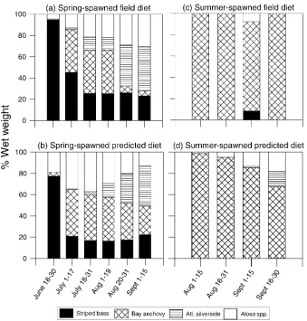
Model-predicted diets of spring- and summer-spawned bluefish demonstrated seasonal patterns similar to those observed in the lower Hudson River during the summer months of the baseline years of 1990, 1992, and 1993 (Figure 4). As observed in field-caught bluefish, the dominant prey of simulated
spring-spawned bluefish showed a seasonal progression from striped bass to bay anchovy to Atlantic silversides (Figure 4a, b). Simulated and observed summer-spawned bluefish diets were dominated by bay anchovy (Figure 4c, d). Predicted contribution of herring to the diets of both spring- and summer-spawned bluefish tended to be overestimated by the model. The predicted range of herring contribution for simulated spring-spawned bluefish was 13–37% versus 5–30% observed in the field data, and the predicted range for herring contribution to simulated summer-spawned bluefish was 1–18% versus less than 8% observed in the field data.
Corroboration.—Once bluefish and prey length distributions and bluefish diets were deemed reason-able, we examined other model prediction variables as part of model corroboration. Under baseline conditions, spring-spawned bluefish displayed consumption rates similar to those observed in recent laboratory and field studies (Figure 5). Predicted consumption rates in
TABLE2.—Mean lengths of prey fish species predicted by the model under baseline conditions compared with observed mean
lengths in long-term field surveys. Field data for striped bass, bay anchovy, andAlosaspp. were from the Hudson River Estuary Monitoring Program for 1984–1996; bay anchovy length data were only collected during 1993–1996. We used American shad
Alosa sapidissima as a representative for the Alosa spp. Atlantic silverside data are from New York Department of Environmental Conservation beach seine samples for 2001–2002. Bay anchovy and Atlantic silversides generally occur at very low abundances in June and thus were not introduced into the model until July.
Prey fish species
Month
Jun Jul Aug Sep
Model Field Model Field Model Field Model Field
Striped bass 23.7 23.7 37.9 43.5 62.1 64.0 86.5 76.3
Bay anchovy 25.9 28.5 34.4 35.9 42.8 40.3
Alosaspp. 36.1 35.3 41.9 49.6 55.0 56.9 70.3 73.7
Atlantic silversides 65.5 68.8 75.3 72.2 85.6 80.8
Figure 5 were obtained by averaging consumption rates over model individuals that were assigned to weight intervals throughout the baseline simulation. Similar to empirically derived consumption rates, modeled blue-fish consumption rates declined rapidly as body weight increased from 1 to 30 g and then leveled off at 0.05– 0.10 g preyg bluefish1d1for bluefish heavier than 50 g.
Prey lengths consumed by bluefish in the baseline simulation conformed closely with prey lengths re-covered from field-collected bluefish stomachs (Figure 6). Empirical diet information was available for bluefish between 50 mm and 200 mm TL. For bluefish in this length range, model-predicted lengths of bay anchovy eaten showed good agreement with bay
anchovy lengths recovered from field-collected blue-fish stomachs (Figure 6a). Predicted and observed minimum anchovy lengths eaten were between 10 and 20 mm TL for all bluefish, and the predicted and observed maximum length of anchovy eaten increased with bluefish length. Model-predicted lengths of bay anchovy eaten did not include as many large (.60 mm TL) individuals as seen in field bluefish diets. Predicted TL of striped bass prey eaten also agreed with field-reported values; predicted and observed minimum striped bass TL ranged between 10 and 40 mm and maximum TL ranged between 30 and 85 mm. Both minimum and maximum striped bass TLs consumed were highly dependent on bluefish length (Figure 6b).
Model Simulation Experiments
We performed three simulation experiments to explore the effects of variable prey fish dynamics on age-0 bluefish growth and the potential for interaction between spring- and summer-spawned bluefish co-horts. The three experiments were designed to assess the effects of variation in prey density alone, in prey timing alone, and in bluefish cohort density and arrival timing. Model input values were varied from their baseline values roughly based upon empirical data collected in the lower Hudson River. Among years in the NYDEC and HREMP surveys, peak prey densities have varied between 5- and 10-fold and prey arrival times have varied by about 30 d. Bluefish dynamics also demonstrated comparable interannual variation by having 5–10-fold differences in CPUE estimates and up to 20-d differences in estuarine arrival timing (Nyman and Conover 1988; McBride and Conover 1991; Buckel and Conover 1997; Buckel et al. 1999a). In the simulation experiments, we varied prey and bluefish densities (650%) from baseline densities and arrival timing (610 d) from baseline arrival times. The arrival time and density of herring were maintained at baseline conditions for all simulation experiments because available empirical data indicated that herring prey represented a minor but stable contribution to bluefish diets across years (Buckel et al. 1999a).
Simulation experiment 1: prey timing.—The first simulation experiment evaluated the effects of variable prey timing by altering the initial appearance of striped bass, Atlantic silversides, and bay anchovy from baseline values (610 d). All 27 factorial combinations
of three appearance times (10 d, baseline,þ10 d) for each of three prey fish species were evaluated. We report the results for the extreme combinations of all three prey species 10 d earlier and all three prey species 10 d later. The other simulations had effects in-termediate to these two extreme cases. This simulation experiment was designed to account for the potential for environmentally generated variation in spawning period and timing of inshore movements of prey fish populations independent of environmentally driven variation in the dynamics of offshore-spawned bluefish cohorts. Offsetting the timing of the initial appearance of prey fishes effectively produced variation in predator–prey body size relationships and in the relative densities of prey species experienced by the bluefish cohorts.
Simulation experiment 2: prey density.—The second simulation experiment evaluated the effects of variable prey density by increasing and decreasing the initial
FIGURE5.—Bluefish consumption rate6SD expressed as
a function of body weight. The results of several past field and laboratory studies (open symbols) are compared with baseline model-predicted consumption (filled circles). Model estimates represent individual bluefish consumption averaged for each 10-g weight increment up to 50 g and for each 50-g weight increment thereafter.
densities of striped bass, Atlantic silversides, and bay anchovy by 50% from their baseline values. As with the first experiment, all 27 factorial combinations of three initial densities (50%, baseline,þ50%) and three prey fish species were evaluated. We report the results of two of the simulations: (1) bay anchovy density at 50% lower than baseline and (2) bay anchovy at 50% lower density combined with striped bass and Atlantic silversides at 50% higher densities than baseline. These two combinations were selected because the altered bay anchovy density alone illustrated the major role of bay anchovy to growth of summer-spawned bluefish, and the simulation with increased striped bass and Atlantic silverside densities showed that the growth consequences of decreased bay anchovy density could not simply be offset by higher densities of the other prey species.
Simulation experiment 3: bluefish density and timing.—The third simulation experiment involved simultaneous variation of the arrival timing and density of the spring- and summer-spawned bluefish cohorts. Three mini-experiments were performed to keep the many possible combinations of initial densities and arrival times for each of the two cohorts to a manage-able level. The three mini-experiments evaluated the potential for one bluefish cohort to indirectly affect the growth of the other cohort through prey consumption. Estuarine arrival times of each bluefish cohort were allowed to vary by610 d from baseline values, and initial cohort densities were varied by650%.
The first mini-experiment (simulation experiment 3a) consisted of nine simulations that examined each possible combination of spring- and summer-spawned bluefish initial density (50%, baseline, andþ50% for each bluefish cohort) with arrival times of each cohort at baseline conditions. The second mini-experiment (simulation experiment 3b) also consisted of nine simulations that examined each possible combination of spring- and summer-spawned bluefish arrival timing (10 d, baseline,þ10 d for each bluefish cohort) with initial densities of each cohort at baseline conditions. The third mini-experiment (simulation experiment 3c) was designed to explore the effects of simultaneous variation in initial bluefish cohort densities and arrival times. We first examined four combinations of early and late summer-spawned cohort arrival (10 d and
þ10 d) with low and high initial densities of the spring-spawned cohort (50% andþ50%). Results from these four combinations yielded a counterintuitive outcome in which early arrival (i.e., longer growing season) of the summer-spawned cohort resulted in shorter average lengths when combined with high initial densities of spring-spawned bluefish. Given this outcome, we then performed an additional six simulations to determine
whether there were conditions that included high initial density of the spring-spawned cohort under which the counterintuitive outcome could be reversed. These six additional simulations were early and late arrival of the summer-spawned cohort each combined with low initial density of the summer-spawned cohort, early arrival of the spring-spawned cohort, and late arrival of the spring-spawned cohort.
Results
Simulation Experiment 1: Prey Timing
Variation in the timing of prey appearance produced only moderate effects on the length frequency distribution of bluefish at the end of the summer. We present model results for the two most extreme conditions of the first simulation experiment, when all three prey fish species appeared in the estuary either 10 d earlier or 10 d later than baseline conditions (Figure 7). When all prey fish were introduced early (Figure 7b), both spring- and summer-spawned blue-fish cohorts reached slightly longer average lengths by October 1 than occurred under baseline conditions (spring-spawned cohort: 261 versus 248 mm TL; summer-spawned cohort: 159 versus 154 mm TL). Similarly, when all prey fish were introduced 10 d late (Figure 7c), both bluefish cohorts showed shorter mean lengths on October 1 than occurred under baseline conditions (spring-spawned cohort: 232 versus 248 mm TL; summer-spawned cohort: 145 versus 154 mm TL).
The effect of delayed prey appearance on the shape of the bluefish length frequency distribution on October 1 was considerably more pronounced for the spring-spawned cohort than for the summer-spawned cohort. The shapes of the length frequency histograms on October 1 for summer-spawned bluefish were similar for the delayed prey and baseline simulations (black bars in Figure 7a, c). In contrast, delayed prey caused a change in the shape of the length frequency histogram for the spring-spawned cohort to include more small individuals (gray bars in Figure 7a, c). Delayed prey species resulted in about 25% of the spring-spawned bluefish having October 1 lengths less than 200 mm and only about 7% of the bluefish having lengths exceeding 260 mm. Under the baseline simulation, only about 7% of the spring-spawned bluefish had October 1 lengths that were shorter than 200 mm and about 25% of the bluefish had lengths that were longer than 260 mm.
Simulation Experiment 2: Prey Density
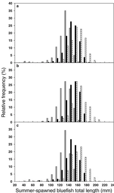
length distributions demonstrated that the spring-spawned cohort was relatively robust to fluctuations in prey fish densities and that bay anchovy played a major role in the growth dynamics of the summer-spawned cohort (Figure 8). A 50% reduction in the initial density of bay anchovy resulted in a 50% decrease in mean length of summer-spawned bluefish on October 1; the majority of individuals in the cohort displayed negligible growth during the summer (Figure 8b). The spring-spawned bluefish cohort was less affected by reduced bay anchovy density, but its October 1 length frequency distribution was strongly skewed to the left because of a small segment of the cohort that displayed much reduced growth (Figure 8b). A 50% increase in the densities of striped bass and Atlantic silversides did little to offset the effects of lowered bay anchovy density (Figure 8c).
Simulation Experiment 3: Bluefish Density and Timing
Variation in the initial densities and arrival timing of the spring- and summer-spawned bluefish cohorts had
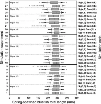
negligible effects on growth and the lengths attained by the spring-spawned cohort. Figure 9 shows the October 1 length distributions for the spring-spawned cohort for all simulations in the three mini-experiments (simula-tion experiments 3a–c). The strongest effects predicted for the spring-spawned cohort occurred when high initial density of the spring-spawned cohort was coupled with either a high initial density or an early arrival of the summer-spawned cohort, resulting in left-skewed October 1 length distributions that included several fish shorter than 175 mm TL (Figure 9; simulations 9, 21, and 27).
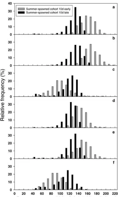
Simulations that varied only the initial densities of the spring- and summer-spawned cohorts (simulation experiment 3a) revealed that the summer-spawned cohort grew more slowly with high initial densities of the spring-spawned cohort (Figure 10). With the spring-spawned cohort at baseline or low initial densities, variation in the initial density of the summer-spawned cohort had little effect on summer bluefish growth and October 1 length frequency distributions (Figure 10a, b). However, growth of the summer-spawned cohort was negatively impacted by high initial density of the spring-spawned cohort; average length of the summer-spawned cohort on
FIGURE8.—Model-predicted length frequency distributions of spring- and summer-spawned bluefish on October 1 for simulations that varied prey fish densities (simulation experiment 2). Model predictions are illustrated for (a) baseline conditions, (b) a 50% reduction in bay anchovy density, and (c) a 50% reduction in bay anchovy density combined with 50% increases in the densities of striped bass and Atlantic silverside prey.
FIGURE7.—Model-predicted length frequency distributions
October 1 was reduced by more than 30 mm (Figure 10c). The impact of a dense spring-spawned cohort on the summer-spawned cohort was amplified if the summer-spawned cohort was itself denser than baseline (gray bars versus black bars in Figure 10c); average length of the summer-spawned cohort on October 1 was shorter than 90 mm. Low initial density of the summer-spawned cohort partly offset the effects of a high initial density of the spring-spawned cohort, allowing the summer-spawned cohort to achieve lengths close to baseline lengths (hatched bars in Figure 10c versus black bars in Figure 10a).
The effects of variation only in the arrival timing of the spring- and summer-spawned cohorts (simulation experiment 3b) on fall lengths of the summer-spawned cohort were moderate and directly related to the length of the growing season (Figure 11). With the spring-spawned cohort at baseline arrival timing, early arrival of the summer-spawned cohort resulted in longer lengths on October 1 and delayed arrival resulted in shorter lengths on October 1 (Figure 11a). When combined with early and late arrival by the summer-spawned cohort, the arrival time of the spring-summer-spawned
cohort had little effect on the growth and fall lengths of the summer-spawned cohort (Figure 11a–c).
Variation in the density of spring-spawned bluefish interacted strongly with the estuarine arrival timing of the summer-spawned cohort to produce large growth effects for the summer-spawned cohort (simulation experiment 3c). At baseline and low spring-spawned cohort densities, summer-spawned bluefish reached longer lengths when they arrived early and shorter lengths when they arrived late (Figure 12a, b). However, at high initial densities of the spring-spawned cohort, early-arriving summer-spring-spawned
blue-fish grew more slowly compared with later-arriving bluefish (gray bars shifted to the left of black bars in Figure 12c). Both length frequency distributions were skewed; a few early-arriving bluefish grew very well compared with most of the cohort, and a few late-arriving bluefish grew poorly. At high densities of the spring-spawned cohort, average length of summer-spawned bluefish on October 1 was 119 mm for the late-arriving cohort and 103 mm for the early-arriving cohort.
We completed six additional simulations to identify potential conditions that might offset the influence of high initial density of the spring-spawned cohort on fall
FIGURE 10.—Model-predicted length frequency distribu-tions of summer-spawned bluefish on October 1 for simulations that allowed spring- and summer-spawned bluefish cohort densities to covary (simulation experiment 3a). Panels represent conditions of differing spring-spawned bluefish density as follows:(a)baseline,(b)a 50% decrease, and (c) a 50% increase. For each level of spring-spawned bluefish density, three levels of simulated variation in summer-spawned bluefish density are represented: baseline (black bars), a 50% decrease (hatched bars), and a 50% increase (gray bars).
lengths of the summer-spawned cohort (Figure 12d–f). Low initial density of the summer-spawned cohort restored the effect of summer-spawned bluefish arrival timing observed at baseline spring-spawned cohort densities, where early-arriving summer-spawned blue-fish reached longer lengths than late-arriving
summer-spawned bluefish (gray bars shifted to the right of black bars in Figure 12d). However, lowered initial density of the summer-spawned cohort did not completely offset the influence of high initial density of the spring-spawned cohort, as fall lengths of the summer-spring-spawned cohort were still shorter than those achieved under baseline conditions (Figure 12a, d). Early arrival by the spring-spawned cohort also served to offset the influence of high initial density of the spring-spawned cohort, allowing early-arriving summer-spawned blue-fish to reach longer lengths than late-arriving summer-spawned bluefish and with length distributions that approached those predicted under baseline densities (Figure 12a, e). However, late arrival by the spring-spawned cohort further augmented the influence of high initial density of the spring-spawned cohort on growth of the summer-spawned cohort (Figure 12f). Under conditions of a high initial density and late arrival of the spring-spawned cohort, early-arriving summer-spawned bluefish grew very slowly (gray bars in Figure 12f). Late-arriving summer-spawned bluefish also grew slowly but were less affected than the early-arriving bluefish (black bars in Figure 12f). Under a high initial density and late-arriving spring-spawned cohort, the average length of summer-spawned bluefish on October 1 was 90 mm for the early-arriving cohort and 112 mm for the late-arriving cohort.
Discussion
Influence of Bay Anchovy Dynamics
The availability of appropriately sized fish prey is an important factor influencing juvenile growth rate and recruitment for both freshwater (Buijse and Houthuij-zen 1992; Parkos and Wahl 2000) and marine (Shoji and Tanaka 2003) piscivores. Our modeling results showed that the growth rates of summer-spawned bluefish were very sensitive to bay anchovy density; lowered bay anchovy densities resulted in October 1 summer-spawned bluefish lengths that averaged nearly 80 mm shorter than lengths under baseline conditions (Figure 8). In model simulations and in field data, the diet of summer-spawned bluefish was dominated by bay anchovy, which often constituted greater than 80% by weight of the total prey eaten (Figure 4; Juanes and Conover 1995; Buckel 1997; Buckel et al. 1999b). Even with higher-than-baseline densities of alternative prey fish species, such as striped bass and Atlantic silversides, predicted fall lengths of summer-spawned bluefish were still shorter than baseline lengths (Figure 8c), further demonstrating the reliance of the summer-spawned cohort on bay anchovy.
Our estimates of bay anchovy density used in model simulations were based upon two independent
term data sets collected during 1984–1996 (HREMP) and 1985–2000 (NYDEC). These surveys involved multiple gears (seines, epibenthic sleds, midwater tucker trawls) in nearshore, shoal, and channel habitats of the lower Hudson River. The use of comprehensive long-term data sets allowed us to obtain good estimates of seasonal and interannual variation in bay anchovy relative densities in a single estuarine system. Howev-er, the accuracy of the absolute density estimates we used in model simulations is more uncertain, given the small body size, high mobility, and patchy distributions of pelagic, schooling forage fish species (Freon and Misund 1999). Different methods used to estimate forage fish densities can produce variable results (Carscadden et al. 1994). For example, Wang and Houde (1995) found that hydroacoustic surveys pro-duced estimates of bay anchovy densities in the Chesapeake Bay that were 2.3–57.7 times higher than densities estimated from comparable trawl surveys. Our baseline bay anchovy densities were within the broad range of densities observed in the Hudson River long-term data sets and in other mid-Atlantic estuaries (Vouglitois et al. 1987; Wang and Houde 1995) and are probably low, given that the field density estimates already include losses resulting from bluefish pre-dation. Although uncertainty exists in the estimates of bay anchovy absolute densities, we are confident that the level of variability (650%) in bay anchovy (and other prey fish) densities that we imposed during simulation experiments was well within the range of natural variation. The variability we simulated was probably more conservative than the two- to fivefold levels of interannual variation in relative bay anchovy density observed in the lower Hudson River and the order-of-magnitude fluctuations in bay anchovy abun-dance seen in other mid-Atlantic estuaries (Vouglitois et al. 1987; Newberger and Houde 1995). Bluefish cohorts probably experience more extreme annual fluctuations in bay anchovy availability than we explored in our simulations.
Previous field studies have noted that the growth rates of summer-spawned bluefish appear to exhibit higher interannual variability than the growth rates of spring-spawned bluefish (McBride and Conover 1991; McBride et al. 1995). In many lake and reservoir systems, which often demonstrate a tight coupling between a small number of top-level predatory species and a few dominant prey fish taxa, prey fish availability plays a major role in regulating foraging success and growth of piscivorous fishes (Olson 1996; Donovan et al. 1997; Michaletz 1998). Although large estuarine systems typically contain a more diverse prey fish community than is seen in freshwater systems, the availability of small forage fishes can be equally
important in determining feeding and growth of estuarine piscivores. The coupling of estuarine pisci-vores with their potential forage species may be especially strong for predators during their first growing season, when small predator body size restricts the size range of susceptible prey. Fitzhugh et al. (1996) hypothesized that low densities of small fish prey led to divergence in growth rates and size bimodality in age-0 southern flounder Paralichthys dentatus; large, fast-growing southern flounder showed a higher degree of piscivory than smaller individuals. Our modeling results suggest that even modest fluctuations in bay anchovy prey densities can generate considerable variation in prey consumption and growth realized by summer-spawned bluefish. High interan-nual variability in the density of bay anchovy is well documented throughout the species’ range (Vouglitois et al. 1987; Nelson et al. 1992; Newberger and Houde 1995) and may be attributable to its opportunistic life history strategy that enables rapid population growth under favorable environmental conditions (Winemiller and Rose 1992; Rose et al. 1999). The strong dependence of summer-spawned bluefish on bay anchovy probably exposes summer-spawned bluefish to large interannual fluctuations in prey availability and may be largely responsible for the highly variable growth observed in the summer-spawned cohort.
Robustness of the Spring-Spawned Cohort
summer may serve to buffer spring-spawned bluefish from fluctuations in the abundance of any one prey species. In addition, bluefish have been shown to feed selectively on high-density prey species, indicating the presence of behavioral flexibility to take advantage of dynamically changing prey resources (Juanes et al. 1993; Buckel et al. 1999a).
The largest responses of the generally robust spring-spawned cohort were predicted under variation in prey timing. Based on previous results in freshwater systems (Adams and DeAngelis 1987) and the size dependence of bluefish capture success (Scharf et al. 2003), we initially hypothesized that the timing of prey arrival would have important growth consequences for both cohorts of bluefish. However, advanced or delayed arrival of any single prey species did not have a major influence on the lengths achieved by either spring- or summer-spawned bluefish (results not shown). Al-though the effects were still relatively modest in magnitude, delayed arrival of three prey species caused an increase in the number of shorter bluefish in the fall length frequency distribution of spring-spawned blue-fish (Figure 7c). This slowed growth was a result of limited prey being available for the early and middle subcohorts of the spring-spawned cohort. Keast and Eadie (1985) concluded that a divergence in size over the summer growing season in largemouth bass
Micropterus salmoides was caused by the lack of appropriately sized piscine prey for smaller largemouth bass, while larger largemouth bass demonstrated a higher degree of piscivory. However, spring-spawned bluefish showed a divergence in size only under extreme conditions (all prey delayed in arrival), suggesting that under most scenarios, the effects of prey timing will be of limited importance to the growth of spring-spawned bluefish.
The general lack of importance of prey timing to the growth of both bluefish cohorts as predicted by the model seems reasonable given the features of juvenile bluefish ecology, but it is inconsistent with the strong associations between predator and prey timing that have often been detected in freshwater systems (Keast 1985; Phillips et al. 1995; Olson 1996). Advanced spawning by the spring-spawned bluefish cohort, combined with a diverse prey fish assemblage, may ensure a size match with at least a subset of the prey fish species. Furthermore, varied spawning periods among the prey fishes in mid-Atlantic estuaries result in numerous cohorts of small-sized prey entering these systems during the summer. Summer-spawned bluefish in model simulations also appeared to be robust to variation in prey timing (Figure 7). The summer-spawned cohort relies on bay anchovy, and thus one might expect a more significant impact of variable prey
timing. However, bay anchovy are small in size, are easier to capture than other prey fish species (Scharf et al. 2002, 2003), and produce multiple cohorts from early summer into fall (Vouglitois et al. 1987; Luo and Musick 1991; Zastrow et al. 1991; Lapolla 2001). Therefore, our simulations suggest that spring-spawned bluefish may be shielded from the effects of variation in prey timing by their early spawning and consump-tion of multiple prey species, while the summer-spawned cohort is buffered from variation in prey timing because of protracted summer spawning, small body size, and the relative ease of capture of bay anchovy, their primary prey.
Interactions between Spring- and Summer-Spawned Bluefish Cohorts
The simulated effects of bluefish cohort arrival times alone on the interaction between spring- and summer-spawned cohorts were generally small (Figure 11). When summer-spawned bluefish arrived early, they achieved longer fall lengths; when they arrived later, they achieved shorter fall lengths. This outcome is clearly related to the time fish spend in the estuary (and in the model); early-arriving fish are afforded a longer time period to accumulate growth. In addition, there were little or no observable effects of arrival time on daily consumption and growth rates of the summer-spawned cohort. Despite only modest effects of bluefish arrival timing demonstrated by our model, previous laboratory experiments that simulated a de-layed estuarine arrival found that fall body sizes of age-0 bluefish may be negatively affected by a shorter growing season (Buckel et al. 1998).
between spring- and summer-spawned bluefish cohorts is likely to be high, given the large interannual variability observed in prey fish densities and the high consumptive demand of age-0 bluefish.
When initial densities and arrival times of bluefish cohorts were varied together, model simulations re-vealed strong and unanticipated cohort interactions. The presumed advantages of early arrival for the summer-spawned cohort (as observed at baseline initial bluefish densities) were negated by a relatively dense spawned cohort. When the initial density of spring-spawned bluefish was high, predicted lengths of summer-spawned bluefish in the fall were longer for the late-arriving cohort than for the early-arriving cohort (Figure 12c). Slowed growth in the early-arriving summer-spawned cohort was directly related to bay anchovy density reductions due to high prey demand of the dense spring-spawned cohort. A very small fraction (,5%) of the early-arriving summer-spawned cohort was able to locate adequate prey resources upon estuarine arrival and grow rapidly enough to reach body sizes that allowed exploitation of the other, larger prey fish species, creating a right-skewed length frequency distribution (Figure 12c). The growth advantages of early versus late arrival for the summer-spawned cohort under a high initial density of the spring-spawned cohort were restored if a low initial density of the summer-spawned cohort (Figure 12d) or an early arrival of the spring-spawned cohort (Figure 12e) was also imposed. Both of these additional conditions acted to offset the higher bay anchovy demand of a dense spring-spawned cohort. Our simulation results indicated that covariation in bluefish cohort dynamics (densities and arrival times) can produce complex effects of the spring-spawned cohort on the summer-spawned cohort via their competition for prey.
Data, Model Considerations, and Caveats
The current version of our model has several limitations that should be considered when interpreting our findings. The assumption of a single, well-mixed volume with cumulative distribution functions for realized encounters is a crude approximation to the possible effects of temporal and spatial variation on bluefish encounters with their prey. Our model was also restricted to the four prey fish species that occur most frequently in bluefish diets in the lower Hudson River. Although bluefish in the lower Hudson River feed almost exclusively on the prey species we modeled, alternative fish and invertebrate prey (Fried-land et al. 1988; Juanes et al. 1993, 2001) have been shown to contribute to bluefish diets and growth patterns in this and other mid-Atlantic estuaries. Our incorporation of energetic costs associated with
in-creased swimming velocities, time spent searching, and prey attacks during feeding periods is partially sub-jective owing to a lack of physiological data represent-ing these activities. In addition, our use of a relatively simple foraging and bioenergetics model (e.g., fixed activity multipliers) is subject to many criticisms (Ney 1993). Lastly, even in situations where we had extensive long-term data, such as with prey densities, the extrapolation of relative density to absolute density is subject to uncertainty. We were fortunate to have two previously developed bioenergetics models avail-able (Steinberg 1994; Hartman and Brandt 1995), detailed laboratory information on bluefish foraging (Scharf et al. 2003), and extensive long-term data on prey dynamics from the NYDEC and HREMP surveys. Thus, despite the many limitations, we believe that with proper interpretation, the model can provide a reasonable quantitative link between prey fish dynamics and summer growth of age-0 bluefish.
Our model would benefit from improved data in several areas. Most notably, more complete growth records for spring- and summer-spawned bluefish based on adequate sample sizes and multiple years would enable more thorough model corroboration. Spatially explicit density information for bluefish and their dominant prey fishes would improve the estima-tion of encounter probabilities and would permit more accurate model predictions of bluefish foraging success under varying prey conditions. Targeted laboratory experiments on bluefish metabolism under different levels of activity would help refine the activity portion of the bioenergetics model. Finally, the generality of our conclusions would benefit from application of the model to other data-rich estuaries besides the Hudson River. Although we used Hudson River data exten-sively, we tried to ensure that the model simulations used changes in bluefish and prey dynamics that were applicable to other locations. Confirmation of our conclusions when the model is based on data from other estuaries would greatly increase our confidence that our conclusions in this paper were not overly influenced by nuances specific to the Hudson River.