University of Windsor University of Windsor
Scholarship at UWindsor
Scholarship at UWindsor
Electronic Theses and Dissertations Theses, Dissertations, and Major Papers
2016
Modeling of Free-Surface Flows with Air Entrainment
Modeling of Free-Surface Flows with Air Entrainment
Vimaldoss Jesudhas University of Windsor
Follow this and additional works at: https://scholar.uwindsor.ca/etd
Recommended Citation Recommended Citation
Jesudhas, Vimaldoss, "Modeling of Free-Surface Flows with Air Entrainment" (2016). Electronic Theses and Dissertations. 5738.
https://scholar.uwindsor.ca/etd/5738
Modeling of Free-Surface Flows with Air Entrainment
by
Vimaldoss Jesudhas
A Dissertation
Submitted to the Faculty of Graduate Studies
through the Department of Civil and Environmental Engineering
in Partial Fulfillment of the Requirements for
the Degree of Doctor of Philosophy
at the University of Windsor
Windsor, Ontario, Canada
2016
Modeling of Free-Surface Flows with Air Entrainment
by
Vimaldoss Jesudhas
APPROVED BY:
______________________________________________ Y. Jin, External Examiner
University of Regina
______________________________________________ D. Ting
Department of Mechanical, Automotive & Materials Engineering
______________________________________________ R. Carriveau
Department of Civil & Environmental Engineering
______________________________________________ T. Bolisetti
Department of Civil & Environmental Engineering
______________________________________________ V. Roussinova
Department of Mechanical, Automotive & Materials Engineering
______________________________________________ R. Balachandar, Co-advisor
Department of Civil & Environmental Engineering
______________________________________________ R. Barron, Co-advisor
DECLARATION OF CO-AUTHORSHIP / PREVIOUS PUBLICATION
I. Co-Authorship Declaration
I hereby declare that this dissertation incorporates the outcome of research
undertaken under the co-supervision of Dr. Ram Balachandar and Dr. Ronald M. Barron
from University of Windsor. Dr. Roussinova’s contribution in this research is to the extent
of providing advice in the preparation of the manuscripts catalogued in the next section. In
all cases, I certify that I am the principal author and have had a major role in the preparation
and writing of the manuscripts.
I am aware of the University of Windsor Senate Policy on Authorship and I certify
that I have properly acknowledged the contribution of other researchers to my dissertation.
I certify that, with the above qualification, this dissertation, and the research to
II. Declaration of Previous Publication
This dissertation includes two original journal papers and one conference paper as
listed below:
Dissertation
chapter Publication title/full citation Publication status
Chapter 3
Jesudhas, V., Roussinova, V., Balachandar, R., and Barron, R., (2015) Numerical study of the turbulence characteristics of a submerged hydraulic jump, 36th IAHR World Congress, 28th
June - 3rd July, The Hague, Netherlands.
Presented
Chapter 3
Jesudhas, V., Roussinova, V., Balachandar, R., and Barron, R., (2016) A CFD study of a submerged hydraulic jump using DES, ASCE, Journal of Hydraulic Engineering.
Under review
Chapter 4
Jesudhas, V., Roussinova, V., Balachandar, R., and Barron, R., (2016) CFD study of classical hydraulic jump using DES, ASCE, Journal of Hydraulic Engineering.
I certify that I have obtained a written permission from the copyright owner(s) to
include the above published material(s) in my dissertation. I certify that the above material
describes work completed during my registration as graduate student at the University of
Windsor.
I declare that, to the best of my knowledge, my dissertation does not infringe upon
anyone’s copyright nor violate any proprietary rights and that any ideas, techniques,
quotations, or any other material from the work of other people included in my dissertation,
published or otherwise, are fully acknowledged in accordance with the standard
referencing practices. Furthermore, to the extent that I have included copyrighted material
that surpasses the bounds of fair dealing within the meaning of the Canada Copyright Act,
I certify that I have obtained a written permission from the copyright owner(s) to include
such material(s) in my dissertation.
I declare that this is a true copy of my dissertation, including any final revisions, as
approved by my dissertation committee and the Graduate Studies office, and that this
dissertation has not been submitted for a higher degree to any other University or
ABSTRACT
This dissertation deals with the computational study of free-surface flows with air
entrainment. The aim of the study was to identify a suitable multiphase flow model that is
capable of not only simulating the intricate flow physics but is also able to capture the
free-surface deformations and predict the air entrainment at a reasonable computational cost.
Finite volume based computations were performed using STAR-CCM+ commercial
solver. The volume of fluid (VOF) multiphase model was used in the present study. First,
a submerged hydraulic jump with an inlet Froude number F1=8.2 is simulated to determine
the capabilities of the VOF multiphase model in capturing the free-surface deformations
and other flow characteristics. The submerged hydraulic jump entrains lesser quantities of
air and the free-surface deformations are not as abrupt as the classical hydraulic jump.
Hence, this problem was chosen as a benchmark to validate the model. The VOF
multiphase model was able to accurately capture the submerged hydraulic jump flow field.
Proper orthogonal distribution (POD) analysis of the fluctuating velocity of the submerged
hydraulic jump revealed the breakdown of large-scale structures into smaller-scale
structures by the interaction of the roller and wall-jet flow, leading to the dissipation of
energy.
Subsequently, a classical hydraulic jump with inlet Froude number F1=8.5 was
studied using the VOF multiphase model. The mean and unsteady features of the classical
hydraulic jump were predicted accurately by the VOF multiphase model. Quadrant
decomposition of the Reynolds stresses revealed that the outward and inward interactions
towards the free surface, leading to interfacial aeration. The VOF multiphase model
over-predicted the air concentration in the classical hydraulic jump due to numerical diffusion.
Further simulations were performed by including a sharpening factor in the formulation of
the VOF multiphase model to contain the numerical diffusion. It was demonstrated that the
air concentration showed that the air concentration distributions in a classical hydraulic
DEDICATION
“The fear of the LORD is the beginning of wisdom: a good understanding have all they
that do his commandments: his praise endureth for ever.”
- KJV, Psalm 111:10
ACKNOWLEDGEMENTS
I would like to extend my heartfelt gratitude and appreciation to my advisors Dr.
R. Balachandar and Dr. R.M. Barron for their guidance, support and benevolence
throughout the course of my study. They have not only been a source of great inspiration
but also a role model that I intend to pursue throughout my career.
I would like to sincerely acknowledge the members of my doctoral committee, Dr.
D. Ting, Dr. R. Carriveau, Dr. T. Bolisetti and Dr. V. Roussinova, for their valuable time
and for consenting to be a part of my doctoral committee. I would also like to thank all my
colleagues for their inquisitiveness and thought provoking discussions that provided an
enriching environment to work in.
A special thanks to my wife for her trust, support, encouragement and patience
without which this work would not be possible. I would like to thank all my friends and
relatives for their moral support during the course of my study.
I would like to thank Natural Sciences and Engineering Research Council of
Canada (NSERC) for their financial support for this study. I would also like to gratefully
acknowledge the entrance scholarship and graduate assistantship I received from
TABLE OF CONTENTS
DECLARATION OF CO-AUTHORSHIP/PREVIOUS PUBLICATION iii
ABSTRACT vi
DEDICATION viii
ACKNOWLEDGEMENTS ix
LIST OF FIGURES xiii
NOMENCLATURE xvii
CHAPTER 1 FREE-SURFACE FLOWS 1
1.1 Introduction 1
1.2 Classification of multiphase flows 2
1.3 Relevance of free-surface flows in hydraulic engineering 3
1.4 Energy dissipation in stilling basins 4
1.5 Types of air entrainment in free-surface flows 6
1.6 Motivation for the present study 7
1.7 Overview of the dissertation 9
CHAPTER 2 MODELING FREE SURFACE AND TURBULENCE IN
HYDRAULIC JUMPS 17
2.1 Introduction 17
2.2 General modeling approaches 17
2.3 Volume of fluid (VOF) model 20
2.3.1 Surface tension formulation 22
2.4 Hybrid RANS-LES approach to model turbulence 24
2.4.2 IDDES formulation of the SST k-ω model 30
2.5 Concluding remarks 31
CHAPTER 3 CFD STUDY OF SUBMERGED HYDRAULIC JUMPS
USING DES 33
3.1 Introduction 33
3.2 The model setup 36
3.3 Validation 38
3.3.1 Mean quantities at z/W = 0.167 39
3.4 Three-dimensional features of the flow field 41
3.5 Unsteady flow features 45
3.5.1 Vortex shedding and mechanism of air entrainment 45
3.5.2 Coherent structures 47
3.6 Conclusions 51
CHAPTER 4 CFD ANALYSIS OF CLASSICAL HYDRAULIC JUMPS
USING DES 68
4.1 Introduction 68
4.2 The model 74
4.3 Validation 78
4.4 Results and discussion 83
4.4.1 Toe oscillations 83
4.4.2 Mean flow and turbulence quantities 85
4.4.3 Quadrant analysis 89
4.4.5 Air concentration 94
4.5 Conclusions 95
CHAPTER 5 PREDICTION OF AIR ENTRAINMENT IN HYDRAULIC
JUMPS 115
5.1 Introduction 115
5.2 The model 120
5.3 Validation of flow parameters 121
5.4 Results and discussions 123
5.5 Conclusions 128
CHAPTER 6 SUMMARY AND FUTURE WORK 138
6.1 Summary 138
6.2 Recommendations for future work 141
REFERENCES/BIBLIOGRAPHY 142
LIST OF FIGURES
Fig. 1.1 Types of multiphase flow regimes in a horizontal gas-liquid flow
(adapted from Brennen, 2005)
12
Fig. 1.2 Air-water flows in hydraulic engineering: “white waters”
encountered in (a) bell-mouth spillway of the Lady Bower reservoir,
UK (b) chute spillway of Itaipu dam, Paraguay
13
Fig. 1.3 Classification of hydraulic jumps based on the super-critical Froude
number
14
Fig. 1.4 Types of aeration free-surface flows; (a) local or singular aeration,
(b) interfacial aeration (adapted from Chanson, 1996)
15
Fig. 1.5 Fig. 1.5 Thermal stratification in reservoirs depicting the intake for
the penstock in the Hypolimnion. (adapted from Hu and Cheng,
2013)
16
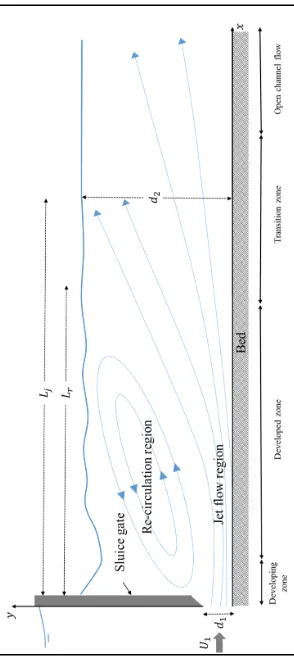
Fig. 3.1 Schematic representation of the flow field in a submerged hydraulic
jump
54
Fig. 3.2 2-D representation of the simulation domain at initial time (t = 0 s) 55
Fig. 3.3 Free-surface profile of the submerged hydraulic jump 56
Fig. 3.4 Profiles of mean streamwise velocity 57
Fig. 3.5 Profiles of mean streamwise turbulence intensity 58
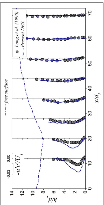
Fig. 3.6 Profiles of Reynolds shear stress 59
Fig. 3.7 Free surface colored with contours of (a) mean x-velocity, (b)
vorticity magnitude, (c) velocity vectors on y/d1 = 5.3 plane
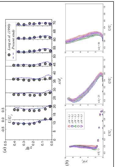
Fig. 3.8 Variation of (a) mean streamwise velocity across the channel at
different streamwise locations, (b) mean streamwise velocity
normal to the bed at different transverse locations
61
Fig. 3.9 Evolution of shear layer at different streamwise locations of the
submerged hydraulic jump
62
Fig. 3.10 Vortex shedding from the sluice gate and air entrainment in the
roller
63
Fig. 3.11 Variation of maximum air concentration in the central plane of the
submerged hydraulic jump
64
Fig. 3.12 Iso-surfaces of 𝜆2colored by contours of z-vorticity 64
Fig. 3.13 Modal distribution of turbulent kinetic energy and spatial
distribution of Reynolds stress for higher order modes in the central
plane
65
Fig. 3.14 Modal distribution of turbulent kinetic energy and spatial
distribution of Reynolds stress for higher order modes in
x d⁄ 1=3 plane
66
Fig. 3.15 Modal distribution of turbulent kinetic energy and spatial
distribution of Reynolds stress for higher order modes in
x d⁄ 1=26 plane
67
Fig. 4.1 (a) Schematic depicting the different zones of flow in a classical
hydraulic jump, (b) typical velocity profile in the developed zone
of the classical hydraulic jump
98
Fig. 4.3 Contours of blending function depicting the RANS and LES
regions
100
Fig. 4.4 Comparison of streamwise velocity fluctuations for the submerged
hydraulic jump
100
Fig. 4.5 (a) Comparison of computed mean velocity with experimental data,
(b) comparison of computed free-surface profiles with
experimental data
101
Fig. 4.6 Similarity analysis of different time-averaged quantities 102
Fig. 4.7 Movement of the toe of the hydraulic jump, superimposed with
contours of z-vorticity
103
Fig. 4.8 Frequency of toe fluctuations (a) Strouhal number vs. Froude
number, (b) Strouhal number vs. Reynolds number
104
Fig. 4.9 Profiles of time-averaged streamwise velocity at different
streamwise locations
105
Fig. 4.10 Profiles of RMS of streamwise turbulence intensity at different
streamwise locations
106
Fig. 4.11 Time-averaged streamwise velocity at different x-z planes 107
Fig. 4.12 Effect of channel aspect ratio on the flow parameters 108
Fig. 4.13 Mean free surface colored by contours of (a) mean streamwise
velocity (b) mean vorticity magnitude
109
Fig. 4.14 (a) Time-averaged Reynolds shear stress at different streamwise
location (b) bed shear stress along the length of the hydraulic jump
110
Fig. 4.16 Vertical distribution of third-order moments at different streamwise
locations
112
Fig. 4.17 (a) Skewness of the streamwise velocity fluctuations, (b) skewness
of the vertical velocity fluctuations, (c) streamwise turbulent kinetic
energy flux, (d) vertical turbulent kinetic energy flux
113
Fig. 4.18 Air concentration at different streamwise locations 114
Fig. 5.1 Schematic representation of the classical hydraulic jump 130
Fig. 5.2 Flow parameters along the center plane of the hydraulic jump (a)
contours of mean velocity (b) velocity vector field (c) mean
Reynolds stresses
131
Fig. 5.3 Decay of mean streamwise velocity 132
Fig. 5.4 Effect of sharpening factor on free-surface profile 132
Fig. 5.5 Effect of sharpening factor on the flow parameters 133
Fig. 5.6 Effect of sharpening factor on the air concentration 134
Fig. 5.7 Fig. 5.7 Variation of (a) maximum air concentration (b) location of
maximum
air concentration long the streamwise direction
135
Fig. 5.8 Distribution of air concentration in different x-z planes 136
NOMENCLATURE
A Area of the control volume
Ai Eigenvectors
an POD coefficients
a1 Constant used in the k-ω SST model
arg1, arg2 Functions used in the k-ω SST model
b Half width of the wall jet
C Time-averaged air concentration at any location in the flow field
Cmax Maximum value of time-averaged air concentration
Cmean Mean air concentration at any given streamwise location.
Cmm Maximum value of mean air concentration for a given x-y plane
C̃ Auto-covariance matrix
CDω Term related to the cross-diffusion term used in k-ω SST model
C'p Co-efficient of pressure fluctuations
Ct, Cl Model constants used in the IDDES model
Cα Sharpening factor used in the VOF model
Dk Dissipation term in the turbulent kinetic energy transport equation
Dω Cross-derivative term in the SST k-ω model
d Depth of flow
dw Distance to the nearest wall
d0 Height of the sluice gate
d2 Tail-water depth
d2* Sub-critical sequent depth
EC Cumulative turbulent kinetic energy
Ek Turbulent kinetic energy associated with each POD mode
F Froude number
F1 Inlet Froude Number
Fku Flux of the turbulent kinetic energy in the streamwise direction
Fkv Flux of the turbulent kinetic energy in the vertical direction
Fn1 Blending function in k-ω SST model
Fn2 Function used in the computation of turbulent time scale
fB Blending function used in the IDDES formulation
fe, fe1, fe2 Elevating function used in the IDDES formulation
ft, fl Functions used in the IDDES formulation
fd,fdt Functions used in the IDDES formulation
fsec Secondary frequency of free-surface fluctuations
ftoe Frequency of toe fluctuations
f𝜎 Surface tension force
fσ,t, fσ,n Tangential and normal components of surface tension force respectively
fβ* Vortex stretching modification term used in SST k-ω model
f Frequency of sluice gate vortex shedding
Gk Turbulent production term
hweir Height of the downstream weir
K Mean curvature of free surface
k Turbulent kinetic energy
k0 Ambient value of turbulent kinetic energy
L Length scale equal to the value of x where Um=0.5 U1
La Length of the aeration
Lr Length of the roller for the submerged hydraulic jump
Lj Length of the submerged hydraulic jump
Lr* Length of the roller of the classical hydraulic jump
Lj* Length of the classical hydraulic jump
lHYBRID Hybrid length scale used in the IDDES formulation of SST k-ω model
N Number of snapshots
p' Pressure fluctuations
Re Reynolds number
rdt, rdl Functions used in the IDDES formulation
S Modulus of mean strain rate tensor
S1 Submergence factor of a submerged hydraulic jump
St Strouhal Number
Sk User specified source terms for turbulent kinetic energy in SST k-ω model
Sr Additional mass source term in VOF model
ST Strain tensor
Su Skewness factor for the streamwise velocity
Sαi Source or sink of the ith phase in the VOF model
Sω User specified source terms for specific dissipation rate in SST k-ω model
t Time
T Time period
Tt Turbulent time scale
U,V,W Mean components of velocity in x,y and z directions
u,v,w RMS values of velocity fluctuations in the x,y and z directions
u',v',w' Fluctuating x, y and z components of velocity
U0 Velocity at the inlet
U1 Velocity at the toe of the hydraulic jump
Um Maximum value of U at any x-location
U' Fluctuating velocity matrix
V Total volume of the control volume
Vi Volume of the ith phase
W Width of the channel
x,y,z Cartesian axis directions
x1 Distance of toe from the sluice gate
y+ Wall normal distance
Greek Letters
α Volume fraction
αi Volume fraction of the ith phase
αdes Function used in the IDDES formulation
γ Blended coefficient of the k-ω SST model
γeff Effective intermittency term in the turbulent kinetic energy equation
γ' Term in the turbulent kinetic energy equation
δt Time step
δ Boundary layer thickness
Δ Distance between cell centers
ΔIDDES IDDES mesh length scale
Δmin Smallest distance between the cell centers
ρi Density of the ith phase
η Free-surface elevation
κ von Karman constant
λi Eigenvalues
λ1, λ2, λ3 First three eigenvalues of (ST2+Ω2)
μ Dynamic viscosity of the air-water mixture
μair Dynamic viscosity of the air
μi Dynamic viscosity of the ith phase
μt Turbulent viscosity
μwater Dynamic viscosity of the water
ρ Density of the air-water mixture
ρair Density of the air
ρi Density of the ith phase
σ Surface tension
σk, σω Inverse turbulent Schmidt numbers
ϕ Set of coefficients used in the k-ω SST model
ϕi POD modes
Ω Rotational tensor
ω Specific dissipation rate
ω0 Ambient value of specific dissipation rate
Tensors and vectors
I Identity matrix
S Stress rate tensor
T Viscous stress tensor
Tl, Tt Laminar and turbulent stress tensors
W Vorticity tensor
u Velocity vector
n Unit normal vector
F Body force term
g Acceleration due to gravity
CHAPTER 1
FREE-SURFACE FLOWS
1.1 Introduction
Multiphase flows are encountered in various applications related to our day-to-day
lives. Some of the common examples include, rain drops falling in the atmosphere,
sediment transport in rivers, oil spills in water bodies, air bubbles in an aerated drink, etc.
In most cases there is no necessity to measure the properties of the individual phases.
However, for applications in petroleum, chemical, and pharmaceutical industries, and in
certain scenarios in hydraulic engineering, it has become increasingly imperative to
determine the properties of the individual phases. A cautionary note about terminology
used in the area of multiphase flows is useful. The term “phase” generally refers to a
“thermodynamic state of matter i.e., solid, liquid or gas”, however, in multiphase flows this
term can be a misnomer as it can be used to describe flows such as oil spill in water, which
is essentially a multi-component or multi-fluid flow. In the current dissertation while
referring to multiphase flows, a more generic definition of phase is adopted and can be
defined as an identifiable class of material that offers a particular inertial response to and
interaction with the flow and the potential field in which it is immersed.
Although the phases present in a flow field can be mixed below the molecular level,
this dissertation only deals with multiphase flows where the phases are mixed well above
the molecular level. This still presents us with a wide spectrum of flow fields. These
multiphase flow fields can be described based on the thermodynamic state of the phases
flow, some of the multiphase flow regimes encountered in horizontal gas-liquid flow is
discussed in section 1.2 and is depicted in Fig. 1.1. However, with the inclusion of the solid
phase, several other flow regimes are also possible.
1.2 Classification of multiphase flows
Topologically multiphase flows can be classified into two distinct types, dispersed
and separated flows. Dispersed flows are flows in which one of the phases is dispersed in
the other continuous phase in the form of bubbles, drops or particulate matter. Separated
flows consist of two or more continuous streams of different phases separated by interfaces.
The multiphase flow regimes depend upon the relative velocities of the individual phases
and also on the orientation of the flow. Some of the multiphase flow regimes (Fig.1.1)
encountered in a horizontal gas-liquid multiphase flow are described below:
(i) Stratified or free-surface flow: These flows involve two or more immiscible
fluids separated by a clearly defined interface, e.g., open-channel flow, sloshing in offshore
separator devices, etc. Such flows occur at comparatively lower liquid and gas velocities.
(ii) Plug and slug flow: These flows show intermittent flow patterns, as they have
alternating regions of high and low liquid concentrations. As the rate of the liquid flow
increases, the liquid becomes the dominant phase and the flow changes from plug to slug,
e.g., large bubble motion in pipes or tanks.
(iii) Bubbly flow: When discrete gas bubbles are present in a continuous liquid it is
referred to as bubbly flow, e.g., air lift pumps, hydraulic jumps, etc. Bubbly flows occur
at high liquid velocities.
(iv) Annular flow: Annular flow occurs at high gas velocities when the gas flows
(v) Mist flow: As the gas flow increases, it picks up liquid from the walls and
incorporates it into the gas flow, this is called a mist flow.
As discussed in chapter 2, identifying the multiphase flow regime is critical in the
choice of the numerical methodology used to model the flow. There is no universal
multiphase flow model that works well in all the multiphase flow regimes.
1.3 Relevance of free-surface flows in hydraulic engineering
Hydraulic engineering deals with the study of the storage, conveyance and flow of
water and other liquids. The open-channel flows that are encountered in hydraulic
engineering are free-surface flows, with an air-water interface. The driving force in
open-channel flows is gravity and there is typically a change in the depth of flow along the
streamwise direction due to the loss of momentum caused by the drag exerted by the bed.
Hence the location of the free surface varies along the streamwise direction. Also, the
free-surface elevation can vary if the flow encounters bumps or other obstacles in its flow path.
The important dimensionless number when studying open-channel flows is the Froude
number defined as F = U⁄√gd, where U is the velocity of the flow, g is the acceleration
due to gravity and d is the depth of flow. In a sub-critical flow (F< 1), the disturbances
of the free surface due to the presence of obstacles tend to travel both upstream and
downstream, while in a super-critical flow (F> 1), the disturbances travel only
downstream. If the Froude number of the flow is equal to one, then a standing wave is
produced in front of the obstacle. These fore-mentioned changes also affect the velocities
in the flow field due to continuity considerations. Hence, when studying open-channel
Energy dissipation in hydraulic structures is another important issue in hydraulic
engineering. When water is discharged from hydraulic structures, the flow has a large
quantity of kinetic energy associated with it. Chute spillways and stilling basin are often
used to dissipate this kinetic energy below hydraulic structures. The failure to dissipate the
energy can result in severe erosion and loss of habitat downstream of the hydraulic
structure. By design, significant quantities of air are entrained in the chute spillways and
stilling basins making the flow two-phase in nature. Fig. 1.2 shows the “white waters”
caused by the air entrainment in (a) bell-mouth spillway of Lady Bower reservoir in
England (b) chute spillway of Itiapu dam, Paraguay.
1.4 Energy dissipation in stilling basins
Stilling basins are hydraulic structures constructed at the base of the spillway to
facilitate the kinetic energy dissipation generally in the form of a hydraulic jump. Hydraulic
jump is a free-surface phenomenon which occurs when a super-critical flow transitions to
a sub-critical flow. Hydraulic jumps are associated with energy dissipation, sharp increase
in free-surface elevation, strong turbulence and air entrainment (Chanson and Brattberg,
2000). The super-critical depth d1 and sub-critical depth d2* are called conjugate depths (see
Fig. 1.3); the ratio of depths is given by the Bélanger equation. The location were the free
surface rises abruptly is called as the toe of the hydraulic jump. The location of the toe
depends upon the tail water depth in the stilling basin. As long as the tail water depth is
less than the sub-critical depth d2* for a given inlet Froude number F1, the toe of the
hydraulic jump occurs somewhere downstream of the sluice gate. This is called as the
classical hydraulic jump. As the tail water depth increases, the toe of the jump moves
sub-critical depth d2* for a given F1 , then the toe of the hydraulic jump gets submerged and it
is called as a submerged hydraulic jump. The flow fields of the classical and submerged
hydraulic jumps are explained in detail in chapter 3 and chapter 4, respectively. The
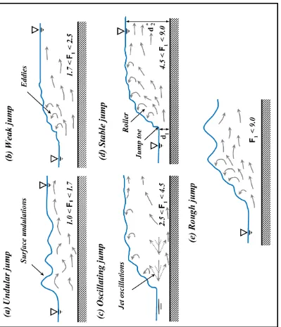
classification of classical hydraulic jump based on the inlet Froude number F1 , depicted
in Fig. 1.3 can be described as follows:
(i) Undular jump: 1< F1<1.7
Hydraulic jumps with inlet Froude numbers between 1 and 1.7 are called as undular jumps,
which are characterized by a slight undulation of the free surface. The difference between
the conjugate depths is not very significant. The recirculation or the roller region is not
formed.
(ii) Weak jump: 1.7< F1<2.5
Hydraulic jumps with inlet Froude number between 1.7 and 2.5 are termed as weak jumps.
Small recirculating eddies appear near the free surface. The loss of energy is not significant
and the ratio between the conjugate depths is of the order of 2 to 3.
(iii) Oscillating jump: 2.5< F1<4.5
Hydraulic jumps with inlet Froude number between 2.5 and 4.5 are known as oscillating
jumps, the jet like super-critical flow emanating from the sluice gate oscillates in the
vertical direction, resulting in surface waves and significant horizontal oscillation of the
toe. The ratio between the conjugate depths is of the order of 3 to 5. A recirculation region
known as the roller is fully developed in this kind of jump, resulting in significant energy
dissipation. However, due to the pressure fluctuations caused by the oscillatory nature of
(iv) Stable jump: 4.5< F1<9
Hydraulic jumps with inlet Froude number between 4.5 and 9 are considered to be the most
stable and are used as energy dissipators below hydraulic structures. The location of the
jump, i.e., the point where the free surface increases abruptly, remains fixed regardless of
downstream conditions. These jumps provide adequate energy dissipation and the rise in
free surface is quite significant with the ratio between the conjugate depths of the order of
6 to 12.
(v) Rough jump: F1>9
If the inlet Froude number increases beyond 9, the jump becomes increasingly rough with
large quantities of air entrained into the flow. This results in colossal sprays, and a very
large size of stilling basins is required to contain the flow. The ratio of conjugate depths
can exceed 20 in this type of jump.
1.5 Types of air entrainment in free-surface flows
Air entrainment aids in the dissipation of energy in hydraulic jumps. The energy is
dissipated due to the shear between air and water and due to turbulent kinetic energy
required to breakup the free surface to initiate the air-entrainment process. Two basic types
of air entrainment processes are identified in free-surface flows (Chanson, 2004).
(i) Local or singular aeration:
This type of air entrainment happens in plunging jets or hydraulic jumps. A singularity or
discontinuity is created at the location where the jet-like flow impinges the surrounding
waters. This singularity is termed as a free-surface cusp (Eggers, 2001). Air gets trapped
(ii) Interfacial aeration:
Interfacial aeration occurs at the air-water interface as shown in Fig. 1.4(b). Air is entrained
into the flow when the turbulent kinetic energy generated in the flow is large enough to
overcome the surface tension and gravity effects. This type of air entrainment can be
observed in chute flows.
Depending upon the type of flow field, air is entrained into the flow by either one
or a combination of both the air-entrainment mechanisms. The entrained air is also
responsible for the bulking of the flow. It is estimated that about 25% of energy dissipated
in stilling basins is due to air entrainment (Hoque and Aoki, 2005).
1.6 Motivation for the present study
From the above discussion it is clear that the free surface, its deformation and its
breakup play an influential role in several problems of practical relevance in hydraulic
engineering. However, when open-channel flows are studied numerically, there is tendency
to use the ‘rigid-lid’ approximation. The free surface is treated as non-deforming and a
free-slip condition is applied on the free surface. This is done to manage the computational
cost and time. However, the ‘rigid-lid’ approximation does not truly reflect the influence
of the free surface on the flow field. Especially in shallow flows, the deformations of the
free surface could influence the velocities throughout the depth of flow (Nasif et al., 2016).
The first objective of the present study is to identify a multiphase flow model that is capable
of modeling the sharp deformations of the free surface with all relevant open-channel flow
parameters encountered in hydraulic engineering with reasonable cost and engineering
Fig. 1.5 shows a typical schematic of a hydropower dam project. The water in the
reservoir, usually consists of two layers, i.e., the top layer called epilimnion and a bottom
layer called the hypolimnion. The epilimnion is well mixed due to the free-surface
turbulence and retains higher dissolved oxygen (DO) due to photosynthesis and exchanges
near the free surface. However, the hypolimnion, contains depleted DO levels due to
animal and plant respiration and bio-chemical oxygen demand. As shown in Fig. 1.5, due
to design considerations, the intake for the penstock pipe is located close to the bottom of
the reservoir, i.e., in the hypolimnion. When water from the hypolimnion with depleted
DO levels reaches downstream, it causes adverse ramifications for the aquatic eco-systems.
In order to increase the DO levels in the downstream flows, the spillway flows are often
adjusted to increase the aeration in the flow. When water is discharged through the
spillway, two mechanisms contribute to increase of DO levels (i) water from the epilimnion
which has higher DO levels mixes with the water from hypolimnion thereby increasing the
overall DO levels, (ii) hydraulic jump occurring in the stilling basin results in the
entrainment of the atmospheric gases into the flow. However, if the reservoir is fully
depleted of DO, then air entrainment through hydraulic jumps remains the only effective
mechanism to increase the depleted DO levels. Alternatively, highly elevated levels of DO
downstream results in supersaturation of dissolved gases and causes gas-bubble disease in
fishes resulting in fish kill (Baxter, 1977). Hence, hydropower projects may have to cease
operations if optimal DO levels are not met downstream of the flow.
Improved prediction of air entrainment occurring in stilling basins will alleviate the
financial impacts caused by the alteration of flow schedules. Though field measurements
they have considerable uncertainties associated with it and they cannot be considered to be
representative of the routinely occurring flow scenario. Another alternative is to use
physical modeling, however air entrainment has scale effects associated with it and cannot
be accurately modeled in a laboratory setup (Chanson and Gualtieri, 2008). Also, the
measuring devices commonly used for air-water measurements have their inherent
limitations making the measurements only relatively accurate (Boyer et al., 2002). The
second objective of the present study is to validate whether the adopted multiphase flow
model is capable of making meaningful prediction of the air concentration in free-surface
flows. Since flow bulking and gas transfer rates are dependent on air concentration, the
model should be effective in scenarios like hydropower projects where prediction of DO
concentrations is vital.
1.7 Overview of the dissertation
In order to realize the above-mentioned objectives, two free-surface flow
problems, i.e., submerged hydraulic jump and classical hydraulic jump were identified and
investigated numerically using multiphase flow models. The submerged hydraulic jump
entrains only moderate quantities of air; however, it provides a benchmark to assess the
capabilities of the volume of fluid (VOF) multiphase model to capture all the relevant flow
features reported in literature. Also, due to its moderate air entrainment, the submerged
hydraulic jump presents the opportunity to carry out higher-order analysis like proper
orthogonal distribution (POD) of velocity fluctuations that are commonly used in
single-phase flows. These higher-order analyses are useful in understanding the internal
micro-structure of the hydraulic jump phenomenon. The classical hydraulic jump represents the
the dominant phenomenon. Hence, the multiphase flow model would be pushed to its limits
to capture the free-surface deformations. Several experimental investigations have reported
the air concentrations in a classical hydraulic jump. Hence, after successfully validating
the flow parameters with experimental results, the air concentration predicted from the
present simulations can be validated. The present dissertation is organized into the
following chapters.
Chapter 2 presents the basis for selecting the VOF model used in the present study.
Also, the present study uses the improved delayed detached eddy simulations (IDDES) to
model turbulence. IDDES uses a combination of Reynolds-averaged Navier-Stokes
(RANS) and large eddy simulation (LES) methods to simulate turbulence. The
hybrid-RANS methodology and its advantages are briefly explained along with the equations for
the IDDES model.
Chapter 3 describes the submerged jump flow field. The free-surface profiles,
velocity, turbulence quantities and Reynolds stresses predicted by the model are compared
with the experimental results of Long et al. (1990). Unsteady flow features such as vortex
shedding from the sluice gate and the mechanism of air entrainment is presented and
discussed. The coherent structures are educed using the λ2-criteria and POD analysis of the
fluctuating velocity field is presented with pertinent discussions.
Chapter 4 describes the classical hydraulic jump flow field. The free-surface
profiles, velocity, turbulence quantities and Reynolds stresses are compared with available
experimental data. The fluctuations of the hydraulic jump toe are captured by the present
simulation. Quadrant analysis of the velocity field and the third-order moments are
Chapter 5 presents the air entrainment characteristics of the classical hydraulic
jump. The use of a sharpening factor in the VOF model to mitigate numerical diffusion is
discussed. The air concentration profiles predicted by the model are compared with the
experimental results. Three-dimensional air concentration distributions in the classical
hydraulic jump are presented for the first time in literature. The three-dimensional
distribution of air concentrations reveals that it is closely related to the velocity field.
F
ig
. 1.1
T
y
pe
s of mult
iphase
flow
r
eg
im
es in a hor
iz
ontal g
as
-li
quid
flow
(a
da
pted f
rom
B
re
nn
en, 20
Fig. 1.2 Air-water flows in hydraulic engineering: “white waters” encountered in (a) bell
mouth spillway of the Lady Bower reservoir, UK (b) chute spillway of Itaipu dam,
F
ig
. 1.3
C
lassific
ati
on of
h
y
d
ra
uli
c jum
ps ba
se
d o
n the supe
r-critica
l F
roud
Fig. 1.4 Types of aeration in free-surface flows; (a) local or singular aeration,
F ig . 1.5 The rma l st ra ti fic ati
on in re
se rvoir s de pi cti ng the intak e for the p ens tock in t he H y poli mni on. (a da pt ed fr
om Hu a
nd C
he
n
g
CHAPTER 2
MODELING FREE SURFACE AND TURBULENCE IN HYDRAULIC JUMPS
2.1 Introduction
This chapter briefly describes the modeling approaches to simulate multiphase
flow. Both the submerged and classical hydraulic jump considered in the present study are
unsteady, turbulent and incompressible two-phase flows. The research reported in this
dissertation is carried out using the STAR-CCM+ (from CD-adapco) commercial solver.
One of the advantages of this commercial code is its ability to tackle problems involving
multi-physics and complex geometries (Nasif, 2014). The Volume of Fluid (VOF)
multiphase flow model is used to model these flow fields. The rationale behind the choice
of the VOF model is provided in this chapter, along with the formulation of the model. The
present study also uses improved delayed detached eddy simulations (IDDES) to model
turbulence. This is a hybrid RANS – LES methodology for modeling turbulence. The
formulation of this methodology from the SST k-ω model is described. The present study
uses the finite volume method (FVM) to discretize the governing equations. It is one of the
most versatile discretization techniques available in CFD. This methodology is described
in Versteeg and Malalasekera (2007), in the STAR-CCM User Guide v8.06 (2013) and
elsewhere, and hence is not presented here.
2.2 General modeling approaches
The term multiphase flow refers to any fluid flow which comprises more than one
phase (term ‘phase’ was defined in chapter 1). A myriad of multiphase flows is encountered
approach depends upon the flow regime that needs to be modeled and also on the physical
properties of the phases involved. The complexity of the multiphase flow model depends
upon the complexity of the physics that the model is expected to capture. Two of the most
commonly used multiphase flow modeling approaches are described below:
(i) Euler – Lagrangian approach:
This type of approach is commonly used for dispersed flows. An Eulerian formulation is
used to model the flow of the continuous phase(s), i.e., the Navier-Stokes equations are
solved for each continuous phase. For the dispersed phase, the Lagrangian approach is
adopted, i.e., equations of motions are used to describe the motion of the individual
particles in the discrete phase. This type of modeling approach provides the detailed
information about the trajectory of each particle and the particle size distribution.
Particle-particle interaction and interaction between the Particle-particles and the continuous phase can be
easily modeled using this approach by adding appropriate force terms to the equations of
motion, such as drag, particle collisions, etc. Any mass transfer between the particles can
also be captured. However, a significant amount of computational power is required to
track all the particles and hence this approach is generally restricted to smaller
concentrations of particles. Also, a considerable amount of post-processing is required to
calculate mean quantities like the void fraction. An example of the Euler-Lagrangian model
is the discrete element method that is employed extensively to model granular material in
(ii) Euler – Euler approach:
In this modeling approach, an Eulerian formulation of the conservation of mass and
momentum equations are solved for each individual phase. The volume fractions of the
phases are tracked separately. A single pressure field is used for all phases. The advantage
of this model is that it can be used for a wide range of concentrations. It also accounts for
the mixing and separation of the phases. The mean quantities can be obtained directly.
However, capturing the individual particles requires a very fine mesh. Particle size
distributions, particle interactions, etc., cannot be modeled directly. Since, the Eulerian
model solves the governing equations for each individual phase, it can be computationally
exhaustive. To reduce computational costs, researchers has developed simplified Euler –
Euler approaches such as the Volume of Fluid (VOF) model. The VOF method treats the
multiphase flow as a mixture and solves a single set of governing equations for the mixture.
This helps to reduce the computational overhead significantly while also yielding results
with acceptable engineering accuracy.
The hydraulic jump is a free-surface phenomenon with sharp deformation of the
free surface. Our first objective is to accurately capture this free-surface deformation. The
VOF model is known to perform well in stratified flows, hence it could be used to model
the hydraulic jump. However, hydraulic jumps have a significant amount of air
entrainment. Experiments have revealed that the nature of the flow is bubbly near the toe
of the hydraulic jump (Chanson and Brattberg, 2000). An extremely fine mesh is required
to capture the individual bubbles in the flow. Nevertheless, the second objective of the
present study is to capture the mean air concentration. This can be computed from the
present study stated here and described in chapter 1, the VOF model appears to be the most
appropriate multiphase model for this research.
2.3 Volume of fluid (VOF) model
The Volume of Fluid (VOF) multiphase model was first proposed by Hirt and
Nichols (1981) and is available in STAR-CCM+. The VOF model is a variation of the
Eulerian-Eulerian multiphase flow model which considers that the immiscible phases
present in a control volume share the same velocity and pressure fields. Therefore, it uses
a single set of equations to describe the transport of mass and momentum for all the phases.
Thus, the equations that are solved are for an equivalent fluid which is a mixture of the
phases present in the flow. The formulation of the model is described in the STAR-CCM+
User Guide v8.06 (2013) and is summarized below. The continuity and the momentum
equations can be written in the integral form as follows:
∂
∂t∫ ρdVV + ∮A (ρu)·ndA= ∫V SrdV (2.1)
∂
∂t∫V ρudV+ ∮A ρu⊗u·ndA = -∮A pI∙ndA +∮A T·ndA + ∫V FdV (2.2)
where Sr in Eq. (2.1) is any other additional mass source terms described by the user, n is
the unit normal vector to the surface element dA, ρ is the mixture density and u is the
instantaneous velocity vector. The two terms in the left hand side of Eq. (2.2) are the
transient and convective fluxes. On the right hand side of Eq. (2.2) are the pressure gradient
term, the viscous flux and the body force terms. Tis the viscous stress tensor, which for a
I is the identity matrix. The body force term F can be any force that might be included in
the study.
The mixture density and viscosity can be calculated as:
ρ= ∑ρiαi i
(2.3)
μ = ∑μiαi i
(2.4)
where αi is the volume fraction of the ith phase defined as Vi⁄V. Here Vi is the volume of
the ith phase and V is the total volume. ρi and μi are the density and viscosity of the ith
phase, respectively. The conservation equation that is solved for the volume fraction is:
∂
∂t∫V αidV+ ∫S αi𝐮 ∙ndA= ∫ (Sαi -αi
ρi Dρi
Dt)
V
dV (2.5)
where Sαi is the source or sink of the ith phase and Dρi⁄Dt is the material derivative of the
phase densities.
The discretization of the transient term in Eq. (2.5) is fairly straightforward,
however for the convective term ∫S αiu∙ndA, the standard discretization schemes are
known not to approximate the large spatial variations of the phase volume fraction. This
can cause smearing of the interface (Rusche, 2002). Hence, to achieve necessary
compression of the interface, an artificial compression term is introduced into the volume
fraction equation (2.5). This term is called the sharpening factor in STAR-CCM+. For a
non-zero sharpening factor, the term
is added to the volume fraction Eq. (2.5), where vciis defined as
vci= Cα|u|
∇αi
|∇αi|
(2.7)
Here, Cα is called the sharpening factor, which can take values between 0 and 1, and u is
the fluid velocity. The sharpening factor can be used to reduce the numerical diffusion of
the simulation due to convection of the step function. If the sharpening factor is set to 0,
there is no reduction in numerical diffusion. If the value is set to 1, there is no numerical
diffusion and a very sharp interface is obtained. This artificial term is only active within a
thin region close to the interface due to the multiplication factor αi(1-αi) in Eq. (2.6).
Therefore, it does not affect the solution significantly outside of this region. However, the
sharpening factor must be used responsibly as it can result in a non-physical alignment of
the free surface.
2.3.1 Surface tension formulation
Another advantage of the VOF model is that it enables inclusion of any other forces
that might be significant for the problem under consideration, through the body force term
in the right hand side of the momentum equation, Eq. (2.2). Dimensional analysis has
revealed that surface tension is an important parameter when studying air entrainment in
hydraulic jumps (Chanson and Gualteri, 2008). Failure to include surface tension in the
simulation can result in over-prediction of air entrainment (Jesudhas et al., 2016). The
methodology employed in STAR-CCM+ to calculate the surface tension can be described
The surface tension force is a tensile force tangential to the interface separating two
fluids. It works to keep the fluid molecules at the free surface in contact with the rest of the
fluid. Its magnitude depends on the nature of the fluids and on the temperature. For a curved
interface, the surface tension force fσ , can be resolved into the normal and tangential
components
fσ = fσ,n+fσ,t (2.8)
where:
fσ,n = σKn (2.9)
fσ,t = ∂σ
∂t t (2.10)
where fσ,n is the normal component and fσ,t is the tangential component of the surface
tension force. Also, σ is the surface tension coefficient, n is the unit vector normal to the
free surface, t is the unit vector in the tangential direction to the free surface and K is the
mean curvature of the free surface. For the present study a constant surface tension
coefficient σ =0.074 N/mbetween the air-water interface was used. When the surface
tension coefficient is constant, the tangential component of surface tension force becomes
zero. The vector normal to the interface is calculated using the volume fraction of the phase
n = ∇αi (2.11)
The curvature of the interface can be expressed in terms of the divergence of the unit
K = -∇∙ ∇αi
|∇αi| (2.12)
Therefore, the expression for the normal component of the surface tension force fσ,n i.e.,
Eq. (2.9) can be re-written as:
fσ,n = -σ∇∙( ∇αi
|∇αi|
) (2.13)
Since, the tangential component of the surface tension force is zero in our present study,
only the normal component of surface tension force is included in Eq. (2.2) to model the
effects of surface tension on the flow field.
2.4 Hybrid RANS-LES approach to model turbulence
Over the years several methodologies have been developed by researchers to model
turbulence in a flow field. The choice of the approach used depends upon the problem
under consideration, computational resources and the purpose of the simulation. At the
very least, the goal of every simulation is to determine the mean quantities of the flow field
with adequate precision. In some cases, the computation of higher-order moments or the
capture of unsteady features of the flow may be required. The Reynolds-Averaged
Navier-Stokes (RANS) models provide a reasonable prediction of the mean quantities with
sufficient engineering accuracy in a majority of flow fields (Casey and Wintergerste,
2000). However, in flow fields dominated by large-scale anisotropic vortical structures,
e.g., wake behind a bluff body, the RANS models yield less than satisfactory results
(Fröhlich and von Terzi, 2008). In such scenarios, large eddy simulation (LES) performs
unsteady characteristics of the flow, which is critical in flow fields where the unsteady
forces must be determined. However, LES is 10 to 100 times costlier than RANS
computations since it requires a finer grid and also calculates the mean quantities by
time-averaging the unsteady quantities over a long sampling time (Fröhlich and von Terzi,
2008). In order to reduce the computational costs and also to adequately capture the
unsteady features of the flow, an endeavor has been made by researchers to combine the
RANS and LES modeling approaches. The objective is to perform LES only where it is
needed and use RANS in regions where it is reliable and efficient.
Another motivation for these hybrid RANS-LES methods comes from wall
bounded flows. In wall bounded flows, the LES concept of resolving the most energetic
eddies results in a significant reduction in the grid size, as the dominating vortical structures
are very small near the wall. As the Reynolds number (Re) is increased, a grid similar to
that for direct numerical simulation (DNS) is required to resolve the flow field (Chapman,
1979). Hence, the LES approach becomes unfeasible for high Re flows. The only way to
circumvent this problem is to use a wall-function near the wall. The use of statistical
information in place of higher resolution is not new to LES as wall functions based on
logarithmic law of the wall has been in use since the early days of LES (Deardorff, 1970).
It is logical to extend this approach by employing a full RANS model near the wall and to
combine it with the LES in the computation of the outer flow.
Though several hybrid RANS-LES approaches are available in the literature, one
of the most prominent and widely used representatives is the detached eddy simulation
(DES), first described by Spalart et al. (1997). It was termed ‘detached eddy’ simulation
employ RANS models in the near-wall regions. The model was first described using the
one equation Spalart-Allmaras RANS model, however, this approach can be extended to
other RANS models as well.
2.4.1 SST k-ω model
The present study uses the improved delayed detached eddy simulation model
(IDDES) available in STAR-CCM+ to simulate both the submerged hydraulic jump and
the classical hydraulic jump. The DES model is suited best in case of flows such as the
hydraulic jump where the turbulence generated at the shear layer between the roller region
and the wall-jet flow region is dominant. The DES model has been used in conjunction
with the SST k-ω RANS model, as it is known to perform better in adverse pressure
gradient flows (Menter, 1992). The formulation of the IDDES version of the SST k-ω
turbulence model, as described by Shur et al. (2008) and in the STAR-CCM+ User Guide
v8.06 (2013), is presented here.
The transport equations for the turbulent kinetic energy k and the specific dissipation rate
ω in the SST k-ω model are:
d
dt∫ρkdV
V
+∫ρuk∙ndA
A
=∫(μ+σkμt)∇k∙ndA
A
+
∫ (γeffGk-γ'ρβ*fβ*(ωkω0k0)+Sk)dV
V
(2.14)
d
dt∫ρωdV
V
+∫ρωu∙ndA
A
=∫(μ+σωμt)∇ω∙ndA A
+∫(Gω-ρβfβ(ω2-ω02)+Dω+Sω)dV V
where Sk and Sω are the user-specified source terms, k0 and ω0 are the ambient turbulence
values in the source terms that counteract turbulence decay, γeff is the effective
intermittency provided by the γ-Reθ transition model, μ and μt are the dynamic and
turbulent viscosities respectively, σk and σω are the inverse turbulent Schmidt numbers and
γ' is defined as,
γ' = min[max(γ
eff,0.1),1] (2.16)
The production of turbulent kinetic energy Gk is evaluated as:
Gk = μt fcS2-2
3ρk∇∙ u -2
3μt(∇∙u)
2 (2.17)
where ∇∙u is the velocity divergence and S is the modulus of the mean strain rate tensor,
S = |S| = √2S:ST = √2S:S (2.18)
and
S = 1
2(∇u+∇uT) . (2.19)
The production of specific dissipation rate ω is evaluated as
Gω= ργ[(S2-2 3(∇∙u)
2)2
3ω∇∙u] (2.20)
where γ is a blended coefficient of the model and S is the modulus of the mean strain rate
tensor given by Eq. (2.18).
Dω= 2(1-Fn1)ρσϖ21
ω∇k∙∇ω (2.21)
where Fn1 is a blending function calculated using Eq. (2.30).
The turbulent viscosity is computed as
μt= ρkT (2.22)
where T is the turbulent time scale.
The turbulent time scale is computed as (Durbin, 1996):
T=min(∝* ω
a1
SFn2
) (2.23)
and S is the modulus of the mean strain rate tensor defined in Eq. (2.18). The values of the
coefficients are taken as ∝* = 1, a1= 0.31.
The function Fn2 is given by:
Fn2= tanh(arg22) (2.24)
where,
arg2= max(2√k β*ωy,
500v
y2ω) (2.25)
and constantβ* has the default value β*=0.09.
The coefficients appearing in Eq. (2.14) and (2.15) are calculated using the blending
function Fn1, such that each coefficient (ϕ)is given by:
The coefficients of set 1 (ϕ1) are:
β1 = 0.0750, σk1 = 0.85, σω1 = 0.5, κ = 0.41, γ1 =
β1 β*-σω1
κ2
√β*
(2.27)
The coefficients of set 2 (ϕ2) are:
β2 = 0.0828, σk2 = 1.0, σω2 = 0.856, κ = 0.41, γ1 =
β2 β*-σω2
κ2
√β*
(2.28)
and, in both Set 1 and Set 2, the constant values are:
β* = 0.09, α* = 1. (2.29)
The blending function Fn1 is defined as follows:
Fn1={
tanh(arg14) without the γ-Re
θ model
max(tanh(arg14), exp[-(ReT
120)
8
])with the γ-Reθ model (2.30)
with
arg1 = min(max( √k 0.09ωy,
500v dw2ω),
2k y2CD
kω
) (2.31)
where dw is the distance to the nearest wall and CDkω is related to the cross-diffusion term,
defined by
CDkω = max(1
ω∇k∙∇ω, 10
-20) . (2.32)
The term fβ* in Eq. (2.14) is a “vortex stretching modification” designed to overcome the
Guide v8.06 (2013) and is set at the default value of 1. Also, near the wall the current
simulations uses the all-y+ wall treatment due to the varying nature of y+ for hydraulic
jumps. This formulation is also available in the STAR-CCM+ User Guide v8.06 (2013).
2.4.2 IDDES formulation of the SST k-ω model
For the IDDES formulation, the dissipation term in the transport equation for k, Eq.
(2.25), is replaced with
Dk =
ρk3 2⁄
lHYBRID (2.33)
where lHYBRID is a hybrid length scale defined as
lHYBRID = fd(1+fe)lt+(1+fd)Cdes∆IDDES (2.34)
Two more functions are introduced to the length scale calculation to add Wall-Modeled
LES (WMLES) capability, a blending function fB and an “elevating” function fe:
fB = min[2 exp(-9αdes2), 1.0] (2.35)
αdes = 0.25 -
dw
∆ (2.36)
fe = max[(fe1-1), 0]fe2 (2.37)
fe1 ={ 2 exp
(-11.09αdes2) if αdes ≥0
2 exp(-9.0αdesα2) if αdes < 0
(2.38)
fe2 = 1.0 - max(ft,fl) (2.39)
ft = tanh[(Ct2rdt) 3
fl= tanh[(Cl2rdl) 10
] (2.41)
rdt=
νt √∇u:∇uTκ2d
w2
(2.42)
rdl=
ν √∇u:∇uTκ2d
w2
(2.43)
Here, Ct and Cl are model constants with values 1.87 and 5.0 respectively, νt and ν are the
eddy viscosity and kinematic viscosity respectively. Also, κ is the von Karman constant
and dw is the distance to the nearest wall. The WMLES and DDES branches of the model
are combined using the function fd as follows:
fd = max((1 −fdt),fB) (2.44)
fdt = 1 - tanh[(Cdtrdt)3] (2.45)
Here Cdt is a model constant of value 20.0. The IDDES model also uses an altered version
of the mesh length scale ∆IDDES, computed as:
∆IDDES = min(max(0.15*d, 0.15*Δ, Δmin),Δ) (2.46)
where Δmin is the smallest distance between the cell centre under consideration and the cell
centres of the neighboring cells.
2.5 Concluding remarks
VOF model is used in the present study to simulate the submerged and classical
hydraulic jump flow fields. Generally, Eulerian models perform well in
stratified/free-surface flows. However, the two-equation Eulerian model is very expensive in terms of the
model treats the flow as a mixture and solves a single set of governing equations for the
mixture, making it computationally less exhaustive than the two-equation Eulerian models.
This is especially useful if simulations must be done on a 1:1 scale for a prototype stilling
basin.
The purpose of this chapter was to present the formulation of the VOF multiphase
model and the IDDES formulation of the SST k-ω model. The VOF model uses other
interface capturing techniques such as the high resolution interface capturing (HRIC)
technique, which is not present here. It is described in the STAR-CCM+ User Guide v8.06