Study of field structure inside a rectangular waveguide corner.

University of Windsor

University of Windsor

Scholarship at UWindsor

Scholarship at UWindsor

Electronic Theses and Dissertations

Theses, Dissertations, and Major Papers

6-1-1970

Study of field structure inside a rectangular waveguide corner.

Study of field structure inside a rectangular waveguide corner.

S. P. Mathur

University of Windsor

Follow this and additional works at: https://scholar.uwindsor.ca/etd

Recommended Citation

Recommended Citation

Mathur, S. P., "Study of field structure inside a rectangular waveguide corner." (1970). Electronic Theses and Dissertations. 6863.

https://scholar.uwindsor.ca/etd/6863

by

S. P. Mathur

A THESIS

SUBMITTED TO THE FACULTY OF GRADUATE STUDIES

THROUGH THE DEPARTMENT OF ELECTRICAL ENGINEERING

IN PARTIAL FULFILLMENT OF THE

REQUIREMENTS FOR THE DEGREE OF

MASTER OF APPLIED SCIENCE

University of Windsor

UMI Number: EC52814

INFORMATION TO USERS

The quality of this reproduction is dependent upon the quality of the copy

submitted. Broken or indistinct print, colored or poor quality illustrations and

photographs, print bleed-through, substandard margins, and improper

alignment can adversely affect reproduction.

In the unlikely event that the author did not send a complete manuscript

and there are missing pages, these will be noted. Also, if unauthorized

copyright material had to be removed, a note will indicate the deletion.

®

UMI

UMI Microform EC52814

Copyright 2008 by ProQuest LLC.

All rights reserved. This microform edition is protected against

unauthorized copying under Title 17, United States Code.

ProQuest LLC 789 E. Eisenhower Parkway

ABSTRACT

Field structure inside a rectangular waveguide corner is

studied. An attempt to calculate the electric and magnetic fields

inside the waveguide in the neighbourhood of the discontinuity region

is presented.

An experimental strategy that is based upon the analogous

behaviour of the acoustic pressure and axial magnetic field is presented.

The technique utilizes holographic interferrometery. Results of some

The author wishes to express sincere thanks to Mr. Philip

Alexander for his guidance and moral support throughout the course of

this work. I would also like to acknowledge the financial help given

TABLE OF CONTENTS

ABSTRACT (ii)

AC KNOWLEDGE EE NTS (ii i )

TABLE OF CONTENTS (iv)

LIST OF TABLES (v)

LIST OF FIGURES (vi)

GLOSSARY OF SYMBOLS (vii)

CHAPTER I INTRODUCTION 1

CHAPTER II THEORETICAL ANALYSIS 5

CHAPTER III THEORY OF THE EXPERIMENT 18

CHAPTER IV EXPERIMENTAL SETUP 36

CHAPTER V RESULTS AN) DISCUSSION 42

CHAPTER VI CONCLUSIONS 45

BIBLIOGRAPHY 46

APPENDIX I 48

TABLE 4. 1 PROPERTIES OF HOLOGRAPHIC PLATES

TABLE 4. 2 DESCRIPTION OF HOLOGRAMS

TABLE 5.1 FIELD COEFFICIENTS

LIST OF FIGURES

FIG. 1 GEOMETRY OF THE RIGHT ANGLE CORNER 8

FIG. 2 PRIMED COORDINATE SYSTEM 14

FIG. 3 RELATION BETWEEN ACOUSTIC AND ELECTROMAGNETIC BOUNDARY 20

CONDITIONS

FIG. 4 GEOMETRY FOR GENERAL DESCRIPTION OF THE HOLOGRAPHIC PROCESS 23

FIG. 5 PRESSURE vs REFRACTIVE INDEX (AIR) 31

FIG. 6 PRESSURE vs REFRACTIVE INDEX (WATER AND WATER AND ALCOHOL 32 MIXTURE)

FIG. 7 ACOUSTIC EXCITATION SYSTEM 38

FIG. 8 SETUP FOR HOLOGRAPHIC INTERFERROMETRY (SCHEME l) 40

a larger dimension of the waveguide

amplitude of the incident wave

A field coefficients

n

b smaller dimension of the waveguide

B field coefficients,

m

c velocity of light in medium of refractive index r|

c velocity of light in air

c velocity of sound

s J

d distance between truncating plane and opposite corner of the waveguide

d distance between opposite corner and intersection of extended waveguide

Ey y-component of the electric field

f frequency of light wave

f acoustic frequency

x-component of magnetic field

z-component of magnetic field

I intensity of stationary image

J zeroeth order Bessel function

o

k propagation constant for light waves

1 length of path of light through the acoustic waveguide

L change in the optical path length

p excess pressure in the waveguide

propagation constant of (1,0) acoustic mode

T transmittance of holographic plate

u particle velocity

U amplitude of acoustic source

v velocity potential

Vq field strength of object beam at recording plate

amplitude of object beam at recording plate

V2 field strength of reference beam at recording plat e

amplitude of reference beam at recording plate

x, y, z cartesian coordinate system

GREEK

|3 propagation constant for (n,0) acoustic mode

1 -9

Cq permittivity of medium, x 10 f/m

p. permeability of medium, 4rr x 10^ h/m

o

X^ light wavelength, 6328 A

A. waveguide wavelength

§

co angular velocity in radians

p density of medium

1-1 GENERAL

The determination of Electromagnetic field configuration in any

region is a solution of Maxwell's equations, formulated either in terms

of a differential equation with appropriate boundary conditions or as an

integral equation which incorporates boundary conditions. The choice

between either method depends on the specific problem.

In the case of waveguide discontinuity problems, an exact solu­

tion by the above methods is very difficult, if not impossible, to obtain.

However, a nearly exact solution can be obtained in most cases by taking

a large number of terms of the series used to express the result.

In the present work, a symmetrically truncated rectangular

waveguide corner is the object of study. The problem is reduced to

2-dimensions by symmetry considerations.

An algorithm for numerical calculation of the field configura­

tion is developed and the computer results are tabulated.

A n experimental strategy to obtain the field structure for

the waveguide is suggested.

1-2 LITERATURE SURVEY

The problem of waveguide discontinuities due to rectangular

corners has been tackled by many workers. M i l e s ^ ^ derived the equiv­

alent circuit of a simple rectangular waveguide corner without

2

used a conformal transformation which carries a bent waveguide into a

straight waveguide filled with non-uniform media. The problem is then

formulated as an integral equation containing a Green's function for

the region. The integrations involved in Rices' work are very difficult

to evaluate and he has not gone beyond the second iteration even for

small angles. Rice obtained approximate formulae for reflection and

transmission coefficients in sharp corners. He did not obtain the field

structure.

(3)

Kao used quasi-optical theory to solve for EM fields in

an overmoded H-plane truncated corner excited by TE^q mode. The diff­

raction effects were, however, neglected in his theory, so that the

comparison of experimental and theoretical results show only fair

agreement.

(4)

Hamid has tried to give the solution to the truncated

waveguide corner problem using Ray theory. However, it must be remem­

bered that Ray methods yield only the first term in the asymptotic

expansion of the modal solution of the total field present in the region

concerned. Even so, the Ray solutions can be changed to mode solutions

by the use of the Poisson sum formula . However, the agreement is only

asymptotic. The method is so complicated that it has only been tried

for parallel-plate waveguide corners.

G o y a l ^ has used the same alternating procedure as adopted

(

6

by Poritsky and Blewett . He assumes appropriate auxiliary fields

for different subregions satisfying the appropriate boundary conditions.

in different subregions. The equations are solved by assuming infinite

series representations for the unknown field components. The results

calculated in terms of the y-parameters of the equivalent network show

good agreement with published data.

Recently, C a m p b e l l ^ ’ has treated the problem of symm­

etrically truncated right-angled corners in the parallel-plate w a v e ­

guide case. The results are also applicable to the rectangular wa v e ­

guide in the TE^q mode of propagation. In these papers he has solved

the general boundary valie problem of a truncated corner. The results

are expressed in terms of y-parameters of the equivalent network for

different d/do values. Standing Wave Ratio (SWR) v s d/do is also plotted.

1-3 PROBLEM FORMULATION

From the literature survey, it can be concluded that although

many workers have tried to solve the problem of waveguide corners, their

main efforts have been in the direction of finding out a suitable equiv­

alent network representation for the specific problem concerned. The

problem taken up in this thesis is that of getting a graphical represen­

tation of total fields inside the symmetrically truncated right angle

waveguide corner. It is believed that this point of view will help in

understanding the behaviour of the 1'corners" in a more complete

fashion. An understanding of this nature could lead to the design of

low SWR (and therefore, low loss) waveguide corners.

In the first part of this thesis (ChapterII), the numerical

algorithm is presented and the results are tabulated. In later sections

4

strategy for obtaining the field structure in the rectangular waveguide.

An indirect technique that makes use of holographic interferrometry

II-l Introduction

Figure 1 shows the geometry of the right angle symmetrically

truncated waveguide corner. As pointed out in sefction (1.2), so far

researchers have been concerned with establishing equivalent network

of the discontinuities from solution of the wave equation with appro­

priate boundary conditions.

The present work deviates from this approach in that the

primary objective here is to obtain the plot of the fields involved.

The system equations are solved to obtain axial magnetic field in the

neighbourhood of, and including the discontinuous region. The total

region is broken up into three sub-regions as shown in fig. 1. The

three sub-regions in this case are not all simple regions in that the

field solution to sub-region II is not available. A numerical algor­

ithm is developed for this sub-region in Section I I -2.

In view of the above discussion it is reasonable to assume

that the field in region II is the vector sum of the fields in sub-

regions I and III if the expressions for fields in region I and III

take into account the effect of the truncating plane i.e. they include

an infinite no. of higher order modes.

II-2 Discontinuity Field Analysis

In this section, solution is obtained for sub-regions I, II

6

i

III

Incident TE^q wave II

>

-y

(9 )

standard and are briefly stated. The numerical a l g o r i t h m for

sub-region II is discussed in some detail.

Since there is no discontinuity in the y-direction, the

electric and magnetic fields will be uniform in the y-direction

i.e. independent of variation in the y-direction.

Furthermore, the waveguide is so designed that only TE^q

mode can propagate in the waveguide so the appearance of higher order

modes will be mainly c o n f i n e d to the discontinuity region. Again,

due to symmetry in the y-directions, it will be assumed that all the

higher order modes will also be TE type.

Therefore, for Region I, near S^;

A Sin (— ) exp (r,z) + A R Sin(— ) exp(-r,z)

1 3 1 . 1 1 3 . 1

+ E~An S i n ( ^ ^ ) exp(F z) (2.1)

n = 2 a n

where

_ r i nrr \ 2 2 - i

r

=

[ T

- u jx e ]

t n L a ’ o o

2 n 2 1 ‘

P. = jfco p e -(-) ] 1 . J o o a J

Other field components are calculated using the following equations

derived from M axwell’s curl equations:

1/2

y n — 2, 3 j • • •

2

(

.

)

Where the superscripts refer to the sub-regions.

In sub-region III, it is assumed that the termination is

matched to the waveguide so that there are no reflections appearing at

i

S 0. T h u s :

= E B Sin (mrT'Z ) exp (-F x) (2.4)

y m=l m a r m

Where

rm = " “ V o 3 1/2 ’ m = I* 2 ’ 3 (2*5)

and the other field components are computed using the following

equations:

r^111 h i i i = _ i _ y

X

, * m

H = - -r2— (2.6)

z jcop. §Z

o

For sub-region II, it is assumed that the fields are vector

coefficients and are calculated by applying the boundary condition

on Ey in sub-region II.

Accordingly, the electric field in sub-region II is given

by:

E11 = E1 + E111 = [A1 Sin (— )(exp(r.z) + R,exp(-F,z))

y y y 1 a 1 1 1

+ E 0 A Sin(^-^)exp(-F z) + S B Sin(— )exp(-f x) 3 (2.7)

n=2 n a n m=l in a m

Equation (2.7) will automatically satisfy the boundary

conditions at and S2 (see fig. l) since the field in sub-region II

is the vector sum of the fields in sub-regions I and III. For instance,

at the contribution of fields in sub-region II due to those of sub-

region I is zero, satisfying the boundary condition at S

At the truncation plane, the boundary condition is:

E11 | , = 0 (2.8)

y 1x+z=a

For simplicity, let the incident TE^q m °de be of unit ampli­

tude, i.e. A^ = 1.; then equation (2.8) becomes:

K1Sin(T )exp(-rli5) + n| 2 An Sin (SES) e x p l - r ^ l + j ^ s l n l ^ l e x p l - r * )

10

Truncating the infinite series in eq. (2.9a) to N terras each;

the number of unknowns in this equation is 2N. Therefore, by applying

eq. (2.9a) to 2N different points on the plane x+z = a; 2N equations

in 2N unknowns are obtained. P and P are calculated using equations

n m

( 2. 2) and ( 2. 5) respectively.

Equation (2.9a) can be written 2N times as:

rrx N N mrrz.

R,Sin( ) exp ( -P z.)+ E „ A Sin (-^^i) exp ( -ri z )+ E.B Sin( ~) exp( -P x )

J. a 1 1 n=2 n a 1 1 m=l m a m l

trx^

-sin( ) exp(riz 1)

a 1 1

rrx„ N Ttrrx N mrrz„

R-sin( )exp(-P z 0)+P A Sin( )exp( -p, z„)+P1B Sin( )exp(-p x„)

J. a 1 1 2 n=2 n a * 1 2 m=l m a r m 2

ttx2

■sin(--- ) exp(riz„)

a 1 2

trx^j N nnx_ N

R sin(— — )exp(-P z )+ EJ1 Sin( )exp(-P z )+ E.B

1 a 1 2N n = Z n a 1 2N m=l :

mrrz „ n x

Sin( )exp(-p x„ )= -Sin( )exp(P1z ) (2.9b)

a r m 2 N a 1 2 N

where x ^ + z ^ = a ; f = 1, 2, 3, ... 2N.

rcl k ] [ ^ ] = -rD i l ] (2.1 0 )

where fC., 1 is a 2N x 2N matrix whose element values are given by: lk

krrx.

C.. = Sin (--- -) exp (-r,Z.)

lk a k i

for i = 1, .... , 2N

k = 1 , a . . . 9 N

and

and

knZ.

C., = Sin(----— ) exp(-r,x.)

lk a k l

(2.1 1)

Pk+N “ r k for k ~ 1 ... N

[x. 1 is a 2N x 1 column vector of unknown field coefficients. Its l

elements are related in equation (2.9) by the following relation:

x i = R i

and [D ] is a 2N x 1 column vector whose entries are given by:

TTX.

D. = Sin(— ~)exp (F,z.)

i a l l

(2.13) f or i = 1, . . . 2N

The solution to equation (2.10) is,formally:

[x] = -[C]-1 [D] (2.14)

Solution for equation (2.14) involves matrix inversion of a complex

2N x 2N matrix, which can be accomplished on a digital computer.

„I ,,111 , _II

T h e n , the e x p r e s s i o n s for E , E a n d E are:

y

y

y

E* = Sin(— ) '*'Z + a 1 sin(— )exp(-F, z) + E ? a sin ( ^ p ) exp(-F z)

v a e 1 a 1 n= 2 n a n

(2.15)

E = E a s m ( )exp(-F x) (2.16)

v •> m a m

ro^l

N

E^1 = [{sin(^) (exp(r^z)+a^exp( -F^z)) an sin^^aT^exp( -I^z) } +

N

{ E , a Sin(^~!exp( -F x)]] ( 2. 17)

1 m a m J

The axial magnetic fields in regions I, III and II are given

as (by use of eqs. (2.2) and (2.5)):

HI = HI = . - i _ i

axial z ^

H1 = - ~~~~ [(-)cos(^) (exp(r..z)+a exp(-F.z) + 2- (^p)

z jcopt u a a 1 1 1 n=Z a

a cost )exp(-F z) ] (2.18)

. n a n

BE111 HIII = Hm = _ J _ y.

axial x

N

IIX 1 t-» /mcrr\ ** /mrrz \ / \ t * r%\

H = --- E (— Jam cos ( )exp(-F x) (2.19)

14

II II

H . , = H , where x 1 , y ' , z' is the new coordinate system

axial x'

is shown in fig. 2.

X

A 0-45

Fig. 2 . Primed Coordinate System

Making the coordinate transformation from unprimed system

to primed system with equations of transformation given by eqs. (2.20);

E'^ is given by (2.21).

x = x 1 cos# + zjsin#

z = z 1 cos# - x Tsin# 4- a (2. 20)

I f # = 45 then

= (x1 + z 1)

/ 2

z = (zT - X 1) -pi + a

and

.N

{ E

m=i m

si n(mrr(:

a / 2

-X1 ) , / (xT+ Z T ) \

+ a) )} (2. 21a)

where

F = + a ) + a 1exp(-ri ^Z^ i; V a) (2.21b)

H"^ can be obtained by applying X

H1^ = T T " 5V (2.22)

X1 JW|J,

o Sz

Therefore with (2.21a) and (2.22), is obtained and then x'

transforming back to the unprimed system of coordinates . in terms 3 XI3 x

of x, y, and z is obtained (given by eq. (2.23))’

H1 1 . . = H11 + j H11 (2. 23)

axial are aim

where

n*1 = rot in [(sin(j3.z) (l-a ) + a cos(j3,z))

(r,

are /2toji u K1 Ire lim ^ 1 a a a

+ E_ exp(-F z)a . (— )cos(— ) - sin(^-^) F ) + F exp(-r x)a .

n=2 n m m a a a n m=l r m mim

/ T T H T / I U l T Z \ ^ ^ . / U U T Z \ i t * \

(— cos ( ) -

r

16

and

r

H^1 = - /k~ r(cos( P z) (l + a . ) + sin(p z) a . (t^- sin(r^) + (rr)

aim J 2wlx - 1 Jre P1 lim 2 a —

o a

cost— )) + exp(-r z)a . (— cost2 3 ) - T S i n ( ^ ) ) +

a n=2 n nre a a n a

E e x p ( - r x ) a (— cos t^3 ^) -r Sint2 2 3 ))] (2.25)

tt=1 m mre a a m a

where second subscripts re and im mean real and imaginary parts respectively

In arriving at equations (2.24) and (2.25) the following relations were

used.

2 TT 2 L/2

r i = % where h = ^ " y ^

" I ^ “ n — 1, ... N a = a +Ja„.

n nre nim

a =? a +ja . ; m = N + l , . . . 2N (2.26)

m mre mim

Equations (2.15) through (2.19) and ( 2.24), ( 2. 25) give

complete field solutions to the problem.

Using the solution method outlined above one can obtain the

field coefficients. The field coefficients values are substituted

in equations (2.18), (2.19) and (2.23) to obtain the axial magnetic

fields near discontinuity, the z-dimension in the input guide can be

taken as 5\g and the x-dimension in the output guide can be taken as

CHAPTER III

THEORY OF THE EXPERIMENT

III-l General

The most commonly used experimental techniques to plot the

electromagnetic fields inside a waveguide consist of small electric

or magnetic probes inserted through slots in the waveguide walls.

These methods are fine except that the probes can appreciably disturb

the fields to be plotted.

suggested here. Before going into the detailed theory of the method

it is relevant to point out the analogue that is suggested as a means

of achieving the desired result. An examination of the wave equation

and its solution in acoustics for pressure variation reveals that there

exists a resemblence between acoustic pressure variation in an acoustic

waveguide and axial magnetic field variation in an electromagnetic

waveguide.

The acoustic wave equation in terms of excess pressure, p,

in three dimensions is given by:

A non-disturbing technique to obtain the field plots is

(3,1) c

for time harmonic fields with boundary conditions

Equation (3.1) applies to a straight waveguide with z axis as

the axis of propagation and rigid walls (normal particle velocity being

zero at perfectly rigid walls.)

Solving equations (3.1) and (3.2) for p gives:

pi v (x, y, z) — P / x cos cos p p exp(-Pz) (3.3)

y ‘vm,n) J o (m,n) a b

rCJ2 . 2-i 1/2 P = propagation constant = + K J

c

For the (l,0) mode the expression becomes:

p (l j0)(x, y, z) - po (ij0) cos (? } exp(_Pl0 z) {3‘4)

where P^^ is the propagation constant for the (l,0) mode. The expression

(3.4) resembles the expression for in the TE-^q mode for the correspond­

ing electromagnetic waveguide:

u „ rTTx'\ -rio z joJt (3.5)

H = H._ cos(— )e 10 e

z 10 a

where the propagation constant for the TE^q wave.

The analogue between pressure field in an acoustic waveguide

and corresponding electromagnetic waveguide will not be complete without

cin investigation of boundary conditions in the two cases. Since a

waveguide termination is used in most practical applications, the follow­

ing discussion on boundary conditions assumes a waveguide with rigid

20

At a perfectly rigid plane wall, the normal component of

particle velocity must be zero and since:

3u _ 1 Bp

Bt £ Bn = 0

we have = 0

Bn

which implies that Bp. 3x

x=0 ,a

Be By

Be

3z = 0 (3.6)

z=0 ,d y=0 ,b

In the electromagnetic guide, the boundary conditions on

H a r e : z BH ___2 Bx x=0 ,a BH ___ 2 By

= o (3.7)

y=0,b z=0 ,d

is not complete since is normal to the wall at z

A comparison of equations (3.6) and (3.7) reveals ttet theanalcgje

0,d. Therefore,

to establish a complete analogue, one has to look at the pressure dis­

tribution at a boundary away from the rigid wall.

Figure 3 illustrates the general idea.

Ideally Free Wall

Z

Y

Therefore, the axial H-field normal boundary condition is

analogues to the acoustic pressure condition occuring a quarter wav e ­

length away from the rigid wall.

Equations (3.4) and (3.5) along with similar boundary condi­

tions on p and clearly demonstrate the analogous behaviour of acoustic

pressure and axial magnetic fields in waveguides. This suggests that

a longitudinal discontinuity in an electromagnetic waveguide can be

studied (in terms of the spatial field distribution) by simply studying

the pressure variations in the acoustic waveguide.

Holographic technique can be advantageously employed for a

study of the analogous acoustic waveguide referred to above. In the

following section, the basic principles of holography are explained.

I l l -2 HOLOGRAPHY

Holography,also referred to as lensless photography, is

essentially a two step imaging process. The first step consists of

recording the interferrogram between a reference and an object beam

(light beam scattered, diffracted or transmitted by the object). After

developing, the interferrogram is placed in the same position as before

and a reference beam is used to view the ''reconstructed'' object. The

object is reproduced by virtue of the reconstruction of the object

beam that has complete information (amplitude and phase) about the

light coming from the object. In the 11 recording'' process, if the

distance traversed by the reference beam and the object beam to the plate

22

phase variations introduced in the object beam by the light coming from

different points on the object itself. In other words, the path

difference introduced between the object and the reference beams (due

to object) is responsible for intensity (amplitude) and phase variations

on the object beam. Next, we consider how such a hologram can be made.

Light waves that are scattered, diffracted or transmitted

by the object impinge on the photographic plate. This light wave

is completely described by its amplitude and phase as functions of

position. The photographic plate will only record the amplitude. To

preserve the phase information, a reference beam, derived from the

same coherent light source, is impinged on the plate. The plate records

the interference pattern between object and reference beams. The inter­

ference will be constructive or destructive according to the relative

phase difference between the object and the reference beams at the

plate thus producing a fringe pattern on the plate. In general, one

can look upon the fringe pattern as a spatial modulation process, in

which the reference beam incident at the photographic plate has

superimposed on it the information that was carried by the object beam.

I l l -3 ANALYTICAL DESCRIPTION OF HOLOGRAPHY^10^

Let £he field strength of object beam at the plate be given

(in complex exponential form) by: (Fig. 4)

Fig. 4

24

where

f'c = ^ is the frequency of the lightwave and and § describe the

amplitude and phase of the light at each position (x, y, z) of the recording

plane. Let the reference beam be:

V 2 = V y, z) exp [j(kx + u>t)3 (3.9)

where k represents the propagation constant in z-direction and is given

2rrcpsft

by . . > 6 is the angle at which the reference beam is incident on the Ac

plate (the angle between the direction of propagation and the normal to

the plate).

The total field at the hologram plane P^ is:

V = Vq+ = [V^ + exp(jkx-j$) 3 exp(j§+jwt)

and the i n t e n s i t y of the recorded field is:

t 2 2

I = J V. V ^ d t ^ V ^ + V ^ + V jV^exp( jkx-j $)+V^V^exp( - jkx+j $) 3

i.e. I = + 2V^V^cos (kx-§)

In the above expression the cosine term indicates that the

spatial amplitude modulation and phase modulation §, are preserved

regard the holographic plate as a (i) detector or mixer to produce a

spatial waveform from a temporal one and (ii) a storage device preserving

the spatial distribution thus produced.

In the reconstruction process, let the reference beam be

incident on the plate. The amplitude transmission through the plate

which is coherently illuminated by V d e p e n d s on the '1 transmittance

cf the plate1T, T. Under normal conditions of photographic processing

T is approximately proportional to the intensity of the exposing radia­

tion i.e.,

T cc I = + ^ ^ 2 cos [kx-§(x, y> z) }

Since the transmitted wave amplitude is given as the product

of the incident wave amplitude and the transmittance, the wave emanating

from the plate illuminated by a replica of the reference beam \ ? 2 i-s:

V. = rv? + V Q2 + 2V V cos(kx-$)}.V0

4 1 3 1 3 2

that is

2 V 1 I

= V^^V-^expJ j<|>)+(V3+— )exp( jlcx)+V1exp(2jkx-j<fi)Jexp( jwt)J (3.10)

Thus, the light emerging from the plate consists of three

te r m s :

26

and thus when sensed by the observer, appears to be coming from the object

(even though the object has been removed). It produces a virtual

image behind the plate.

(ii) The second term is merely the reference beam and can be reduced

by making large as compared to (typically 10 times as large).

(iii) the third term represents the presence of the original wave

with a negative phase term. This implies that, when sensed by an

observer there seems to be a wave propagating ,Ttoward,T a version of

the object. This is the real image of the object,• formed in front of

the plate and it can be viewed or projected on a screen without the

use of additional optics.

The exp(jkx) term merely suggests that the wave leaves the

plate obliquely and thus images will be formed off-axis.

In the above analysis light is described as a cosi nusoidal

waveform implying thereby that it is highly monochromatic and is derived

from a single point radiator i.e., the light has both temporal and

spatial coherence. The light produced by a correctly adjusted laser

is highly monochromatic and spatially coherent. These features make the

laser an automatic choice for the light source in this application.

Next, since the holographic process is essentially an interferrometric

method, components (mirrors etc . ) should be stable. For this reason

all the components have heavy bases and the whole setup is on a stable,

vibration free, flat stone table. This stability requirement on the

III.4 VIBRATION ANALYSIS

The adherence to requirements of stability imposed on compon­

ents and the object itself during the exposure time is vital to obtain

a hologram of the stationary object. A vibrating object can be considered

stationary if the exposure time is much less than the period of vibration

of the object (’’pulse .holography’’). ’’Pulse’’ holography gives infor­

mation regarding the amplitude of vibration at various points of the

object at one particular instant of time.

An extension of the above idea is double-exposure pulse-

holography. Here, two ’’pulse1' holograms are recorded on the same

holographic plate — one with the object in the stationary state, the

other with the object at its peak amplitude of vibration. This type of

hologram can yield information regarding deformation of the surface

of the object due to its motion. The optical path difference between

the two object beams introduced by the motion of the object gives a

fringe pattern in the reconstructed image.

One of the difficulties in ’’pulse holography’’ is that of

synchronization of the laser pulse with the maximum amplitude of vibra­

tion of the object,that is, one must know precisely when to activate

the pulsed laser so as to avoid recording the object going through a

null position. This is difficult to decide in most cases and particularly

so in the case of standing wave in a ’guide.

A further extension of the idea of double exposure pulse

holography is time-average holography. This can be thought of as the

28

or scattering) surfaces distributed along the positions that the actual

vibrating object will occupy during the exposure time. In this type of

holography the exposure time is several cycles of the frequency of

vibration of the object and a continuous wave laser such as a He-Ne

laser is used.

Powell and S t e t s o n ^ ^ described a method for recording

various modes of vibrating objects using time-average holography.

It was shown that each part of the reconstructed image will be degraded

in accordance with the amplitude of vibration of that part of the object.

The intensity of reconstruction and the amplitude of vibration of the

object are related by the zero order Bessel function :

I = J [r“ L 3 x I (3.11)

o St

c

where L is the maximum optical path length change and I is intensity

of the image of the stationary object.

The reconstructed image thus has dark and light fringes

corresponding to the zero and extrema of Jq respectively. These lines

represent the contours of constant amp of vibration.

In order to view the hologram reconstruction (and any of the

interference effects that may occur due to motion of the object during

the recording interval), one must image the wavefronts diffracted by the

hologram when it is illuminated by a suitable replica of the reference

field. One method consists of illuminating the hologram by a wave

time average holography is the amplitude of vibration of the object.

As indicated by equation (3.10) the intensity of the reconstructed

image depends on V which in turn depends on the amplitude of vibration

of the object. A very low amplitude will mean a low phase shift (angular

path difference) between reference and object beams thereby giving a

2rrL

small number of fringes (or no fringes at all if is less than the c

first zero of dQ )* On the other hand, too large ananplitude will

mean a large number of fringes and the extrema will be small in amplitude,

resulting in poor fringe contrast in the reconstructed image.

I l l -5 APPLICATION OF VIBRATION ANALYSIS

The technique of time average holography can be applied to

obtain the fringe pattern in the reconstructed image that corresponds

to the excess pressure field variations that are present in an acoustic

waveguide. The passage of a pressure wave causes the refractive index

of a material to change. This creates an optical path length change

between the two parts of the object beam (one passing through the region

of maximum refractive index change and the other passing through the

region of minimum refractive index change) and a fringe pattern is thus

obtained in the reconstructed image.

Equation (3.1l) shows that the brightness of the reconstructed

image is proportional to the magnitude of the zero order Bessel functions

2ftL

of argument . Since the first zero of J occurs at approximately c

2.40 radians; the minimum phase change, , between two object beams must

correxpond to this value. In order to obtain five to six dark and light

30

One way to obtain the phase shift, §, is to change the optical path

length for the object beam. A change in optical path length can be

affected by changing the optical refractive index of the medium through

1 *

which the beam is passing, since c = — c . As the pressure wave n

travels through the acoustic waveguide the refractive index of the medium

is changed according to the pressure variations in the compressions and

rarefactions of the wave. Actual data shows that the relation between

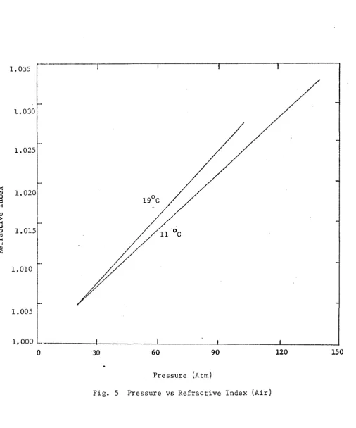
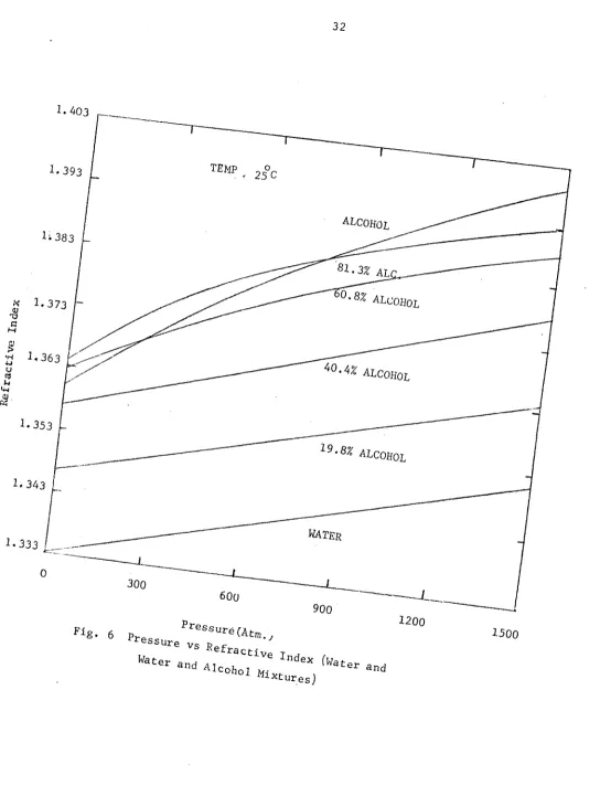
refractive index and pressure is linear for most cases (fig. 5, 6). Thus,

the peak to peak pressure variation in the acoustic waveguide introduces

a change in optical path length of the object beam as it passes through

the waveguide, and hence effects the phase shift, §.

From equation (3.11) we have,

I = J U ) I

o st

2ttL ' _ , or ^ — r $

c

or 2rr (Maximum change in optical path length due to pressure variation) = §

(3. 12a)

Therefore, knowing S, by considerations of fringe number

desired, a maximum change in optical path length can be calculated from

equation (3.12a). The corresponding necessary change in refractive index

R

e

f

r

a

c

t

i

v

e

I

n

d

e

x

1.030

1.025

1.020

19 C

1.015

1.010

1.005

1,000

120

60 90

0 30

Pressure (Atm)

32

1. 4 03

TEMP

M

40 • « a l c o h o l

1 9 -sz ALCOHOL

300

900

Pressure(Atm.;

Fig. 6 Pressure vs Refractive Index (Water and

Water and Alcohol Mixtures)

1200

( 1 2 )

III.6 EXCITATION OF ACOUSTIC GUIDE '

When the acoustic frequency is sufficiently highso that more

than one mode can be propagated in the guide, it becomes necessary to

design a source which will excite only the desired mode. As in the

electromagnetic case, one can design mode filters to allow only one

mode to propagate without special design of the source but as it turns

out, the design of the source is much more convenient to control in

the acoustic case. For this, it is important to realize the conditions

necessary for the exclusion of unwanted modes.

The velocity potential v i-n a lossless semi-infinite rectangu­

lar acoustic guide defined by the planes at y = + a and z = + b

- (12)

and source located at x = 0 is given by

v = v Sin( ^ ^ ) e x p j(wt-p x) (3.13)

n=0 n cos 2a pn

except in the vicinity of the source. Since the source is u = U(y)

exp(jwt), the x dependance can be neglected if frequency f does not

Q g / \

exceed the cut off frequency — of the (0, 1) mode. Also,

"W 2 9 1/2

^n = £(^ ) ” ^^b^ ^ ^or ^n ’ ^ m°de ' (3.14)

V " = t ^ t3.»)

34

(3.15) is zero for any value of n, (i.e. a particular mode), the source

will not excite that mode.

In particular a symmetrical source [u(y) = u ( - y ) 3 w i l l

not excite odd order modes while an an tisymmetrical source will only

excite odd modes.

If the frequency of operation is so adjusted that only (0,0)

and (l,0) modes propagate (i.e. — < f g < ^ ) , then these modes can be

selectively excited by two piston sources operating with equal amplitudes

in phase or out of phase giving conditions of symmetrical and anti-

symmetrical sources described above. Equation (3.15) gives the conditions

for elimination of (0,0) and (1,0) modes as:

+b

J U(y) dy = 0 (3.16a)

-b

and

+b

j

-b

Equation (3.16a) means that the mean strength of the source

should be zero and (3.16b) implies that the source be symmetrical

and have zero strength at the origin.

To excite mode (2,0) free of (0,0) and (l,0) modes, one must

satisfy equations (3.16a) and (3.16b) simultaneously. This can be done

if we have three piston sources; a pair of equal amplitudes and same

phase located at + yQ (where Y0 < b ) and a third at y = 0 in a n t i ­

+b

U(y} CO S (“t") = 0 (3.16c)

-b b

Condition (3.16c) can be achieved by reversing the phase

of the centre source ( ^ p i s t o n ' 1) fchA (l,0) modeiwill still be excluded

since the source remains symmetric.

III.6 EXCLUSIVE EXCITATION OF P MODE 1°

For this mode the sourceatx=0 must be anti symmetrical so

that all the even modes will not be excited by virtue of equations (3.16).

The exclusion of higher (odd) order modes is affected by proper choice

of the frequency f of the transducer (acoustic source). If f is chosen

s s

so that “ < f < then modes (3,0). (5,0) etc. will all be cut off.

6a s ' 4a

Therefore, if two transducers at + yQ (y < b) operating with

equal amplitude but opp. phase are used, the only mode excited will be

(l,0). Small probes may be placed at +b and at origin to monitor the

proper amplitude and phase relationship of the sources. Ideally, the

CHAPTER IV

EXPERIMENTAL SETUP

IV. 1 GENERAL

For mechanical convenience the waveguide dimensions were

chosen to be 7.185 x 3.36 cm.I. D> This corresponds to a cutoff

frequency of 2. 376 kHz for the (ip) mode in air at 18°C and a cutoff wave

length of 14.37 cm. The cutoff frequency for the (0,l) mode is about

5.080 kHz. The mediatised have the property of being colorless and not

reacting with plexiglass, which is the material for the wavegiide. The

length of waveguide was kept at 20 cm. for the straight guide while for

the truncated corner one of the arms, was 20 cm. long. The reason for

this is because of the pressure probes that extend up to app 6 cm, of

the length of the 'guide! Thus the region under observation is relatively

free from distortion introduced by the presence of the probes. The

frequency used was 6.0 kHz.

The vibrations in the walls of the waveguide are kept at a

minimum by making them 1.0 cms. thick (see Appendix I).

I V . 2 ACOUSTIC DESIGN

Based upon equations (3.12a) and (3.12b), the maximum change

required in refractive index, to obtain the phase shift, §, of 13.0 to

14.0 radians in the light beam, is from 13.09936 x 10 ^ to 14.1070 x 10 ^

per cm. of path of light in acoustic waveguide. Expected number of fringes

is about five (corresponding to the number of extremas for Jq in 13.0

The maximum pressure change required to achieve this change

in refractive index (see Fig. 5) for air would be 0.000325 p. bars.

This corresponds to a sound pressure level (SPL) of 140 db. In terms

4

of acoustic power this SPL is approximately equal to 10 watts. Such

high power requirements, if the above computations are to be considered

reliable (an earlier estimate had yielded a lower value), would be

difficult to meet through normal amplification systems. In any event,

attempts have to be directed towards utilizing high power transducers

along with high pressure microphones to generate or monitor the pressure

inside the waveguide.

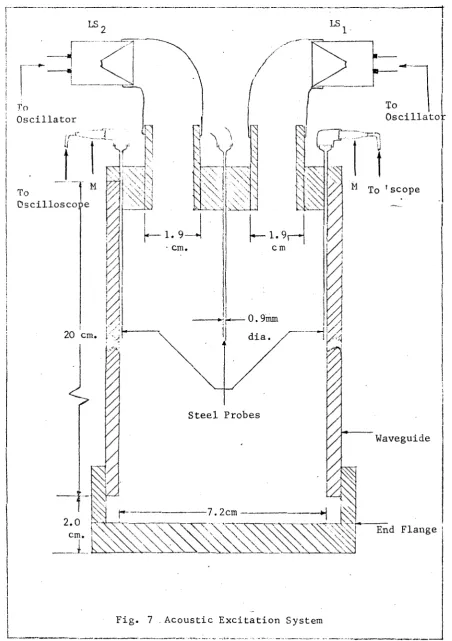
Figure 7 gives the details of the excitation system. This

(

)

is based upon a similar arrangement used by Shaw in an experiment

to determine absorption coefficient of different acoustic materials.

The unsymmetrica1 excitation is achieved by operating two loud speakers

in phase opposition. The excitation for both LS^ and LS^ is derived

from the same source; Oscillator (200 CD HP) which is fed to a stereo

amplifier (80 watt stereo). The phase reverse control on the stereo

amplifier is used to obtain phase opposition between LS^ and L S^

The amplitude controls on chi and ch2 of the amplifier are so adjusted

as to give the same amplification to both channels.

The amplitude and phase of the pressure is monitored by

using two identical B and K microphones (type 4136). The connection

to the respective probes is made by a small flexible rubber tubing. The

length of the two rubber tubes is kept the same and small to have the

38

LS. LS.

! To

Oscillator

To

Oscilloscope

0. 9 mm

20 cm. i _dia.

Steel Probes

7. 2cm

To

Oscillatot

To 'scope

Waveguide

End Flange

The output of the microphones is monitored on a dual beam oscilloscope

for ready comparison.

IV.3 LIGHT SOURCE AND HOLOGRAPHIC PLATES

Since time average holography was to be tried the source of

o

light is a JODON He-Ne laser with A of 6328 A and max power output of

15 mw. A spatial filter is used to ''clean11 the beam and then a beam

splitter (mostly 25 mm. cube type) is used. Wheneverthe mirror type beam

splitter is used, it is placed in front of the spatial filter as shown

in fig. 8.

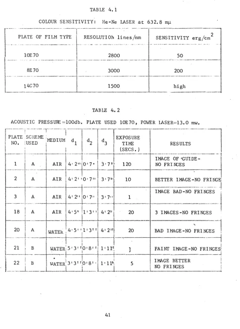
Holographic plates used were SCIENTIA 10E70 and 8E70 plates.

The data on these plates appear in Table (4.1). The 10E70 plates are

high resolution, average sensitivity plates while 8E70 are high resolu­

tion, low sensitivity plates. Film 14C70 is extremely low resolution

and highly sensitive. The 10E70 plates were chosen in view of the max;

power available from laser.

All the optical components used were highly stable and the

experiment was carried out on a stable vibration free, flat surface.

IV.4 EXPERIMENTAL DETAILS

The max. pressure created inside the acoustic guide was 100 db

(for air and water). Figures 8 and 9 represent the general scheme used

for obtaining the hologram. Table 4.2 lists the critical distances

involved, exposure times and remarks on the result of the hologram.

The light beam was incident normally on the waveguide (object) and the

40

OBJECT

SPATIAL FILTER

Ml

EXPERIMENTAL SETUP (SCHEME A) Fi

BEAM SPLITTER

]LASER

OBJECT

SPATIAL \ FILTER

/Ml

Fig. 9. EXPERIMENTAL SETUP (SCHEME B)

PLATE OF FILM TYPE RESOLUTION lines/mm SENSITIVITY erg/cm2

10E70 2800 50

8E70 3000 200

14C70 1500 high

TABLE 4. 2

ACOUSTIC PRESSUIE =100db. PLATE USED 10E70, POWER LASER=13.0 raw.

PLATE NO.

1

SCHEME

USED MEDIUM d i

4' 2"' j ~ J ! d3 EXPOSURE TIME (SECS. ) RESULTS

A AIR 0 1 7" 3' 7" ' 120

IMAGE OF 'GUIDE - NO FRIN3ES

2 A AIR 4' 2' 'O' 7" 3' 7" 10 BETTER IMAGE-NO FRINGE

3

18

A AIR 4' 2" 0' 7" 3' 7" 1

IMAGE BAD-NO FRINGES

A AIR 4'5" 1 • 3 * ' 4' 2" 20 3 IMAGES-NO FRINGES

20 A

WATEk 4 1 5' '1 1 3 ’ ' 4' 2" 20

\

BAD IMAGE-NO FRINGES

21 | B _WATER

*

i

i 5 ' 3 "0 ' 8 "

' .

1' 11" _] FAINT IMAGE-NO FRINGES

22 B

' i |

WATER1 3' 3 ’ '.O' 8' '

_______ ]______ L _

I'll1'! 5

1. ... . ... .

CHAPTER V

RESULTS AND DISCUSSIONS

V.l COMPUTATIONAL RESULTS

The algorithm outlined in Chapter II was used to obtain

numerical results on an IBM 360/50 computer. For the calculation of

elements of matrices C and D a FORTRAN IV programme is used. For inver­

sion of complex matrix C and evaluation of complex field coefficients

(vector x) MATLAN is used.

The results are presented in Table 5-1. (Appendix I I ). The

reflection coefficient for some of the runs are higher than one which

-9

is physically inconsistent. On setting the error criterion at 10 , some

of the results improved, although the difference from the previous results

was only at the sixth decimal place. Setting the error criterion even

-5 "3

higher, at 10 and 10 , the coefficient values changed significantly

but some of the reflection coefficients were still' higher than one. No

trend in the values of coefficients with error settings could be observed.

The reason for inconsistent reflection coefficients is not

immediately obvious. It is possible that the initial assumption made

in developing the algorithum, namely that the field in the subregion II is

vet£or sum of fields in subregions I and III, is responsible for this behaviour.

V . 2 EXPERIMENTAL RESULTS

As indicated in Chapter IV, Table 4.2, the hologram studies

were conducted varying different parameters such as distances involved

and medium in the acoustic waveguide. Although the holograms of stationary

varia-tion in an acoustic waveguide could not be obtained in these runs.

In what follows, some possible reasons for this are briefly

enumerated and discussed:

(i) Acoustic power considerations. It is possible that

acoustic power level may have been too low to create any appreciable

difference in optical path length between two object beams. But on the

otherhand, power levels of the magnitude predicted by theory (section IV-3)

are impractical.

(ii) Acoustic frequency considerations. The choice of acoustic

frequency depends on the following considerations:

(a) A n incorrect choice of frequency might lead to the fringes

in the hologram being washed out. The criterian here is that if the

exposure time is greater than the time required to obtain an optical

phase shift of ninety degrees, between object and reference beams, then

the fringes will be washed out.

A simple calculation shows that for the present choice of acoustic

frequency (6.0 KH Z ) , the exposure time is much less than the time required

to obtain phase shift of ninety degrees between object and reference

beams. In fact high acoustic frequency in the range of several megahertz

is low enough to ensure that the criterian for obtaining the fringes is

not violated.

(b) A low acoustic frequency has the disadvantage that a

corresponding high acoustic power is required to effect the necessary

(optical) refractive index change in the waveguide (as indicated in

require-44

ments to a reasonable level (14).

The problem associated with the use of high frequencies are

two fold - first, the existance of (propagating) higher order modes in

the waveguide and second, the phenomenon of Bragg reflection. Both the

these effects are undesirable since they interfere with the objective

of this experimert;

The frequency used in this set up is a bit low so that high

acoustic powers must be generated. A proper choice of acoustic frequency

seems to be 1.0 M H Z , which gives the advantages associated with high

frequencies while avoiding the disadvantages that might ensue if the

The problem of obtaining electrical and magnetic field structures

inside a rectangular waveguide corner has been investigated from both

theoretical and experimental aspects.

A theoretical analysis of the problem is carried out and field

coefficients have been calculated. Some, of the results display a reflec­

tion coefficient higher than unity. It can be concluded that the approx­

imation used to calculate the field structure is not completely satisfactory.

The reason for this may lie in the assumption that field in discontinuous

sub-region is the vector sum of the fields in the continuous sub-regions.

An experimental method for indirectly obtaining the field structure

is developed based on the analogy between the axial magnetic field in an

electromagnetic waveguide and excess pressure variations in a corresponding

acoustic waveguide. The experimental strategy is charted out. A no n ­

disturbing method (holographic interferrometry) of obtaining excess pressure

variations in the acoustic waveguide is described. Exploratory runs were

made during this investigation in an effort to obtain hologram^of^ above

mentioned pressure fluctuations. Although the results obtained with the

existing equipment fail to display the fringe pattern for an acoustic

waveguide, it is believed that further investigations can overcome the

associated experimental difficulties (as discussed in section V . 2, Chapter V)

and that the strategy presented in this thesisis a workable one.

BIBLIOGRAPHY

1. Miles, J . W . , 1'The Equivalent Circuit of a Corner Bend in a Rectang­ ular Wavegui.de'1 , Proc. I.R.E., Vol. 35, Pp. 1313 - 17, Nov. 1947.

2. Rice, S.O., ''Reflection from Corners in Rectangular Waveguides --Conformal Transformation1', Bell System Technical Journal, Vol. 28,

Pp. 104 - 135, 1949.

3. Kao, K.C., ''Approximate Solution of the 11-Plane Right-Angled

Corner in Overmoded Rectangular Waveguide, Operating in H Mode'', Proc. I E E , Vol. Ill, No. 4, pp. 624 - 628, April 1964.

4. Hamid, M.A.K. , ''An Investigation of Sharp Discontinuities in Rectangular Waveguides by Ray Theory'', International Microwave Symposium, Proceedings, Detroit, Michigan, pp. 39, IEEE cat. no. 68, C38, 1968.

5. Goyal, K . G . , ''Field Structures in Waveguide Corrars'', M.Sc. Thesis, University of Toronto, 1969.

6. Poritsky, H . , and Blewett, M . R . , ''A Method of Solution of Field Problems by means of Overlapping Regions,'' Quarterly of Appl. Math., Vol. Ill, No. 4, Jan. 1946.

7. Campbell, J . J . , ''Applications of the Solutions of Certain Boundary Value Problems to the Symmetrical Form-Post Junction and Specially Truncated Bends in Parallel-Plane Waveguides and Balanced Strip Transmission Lines1', IEEE Trans. M T T , Vol. MTT-16, pp. 165 - 176, March 1968.

8. Campbell J.J. and Jones W . R . ,''Symmetrically Truncated Right-Angle Corners in Parallel-Plate and Rectangular Waveguides'', IEEE Trans. MTT, Vol. MTT - 16, pp. 517 - 529, Aug. 1968.

9. Collin, R.E. , ''Field Theory of Guided Waves'', McGraw - Hill Book Co 1960.

10. Reynolds, G . , and DeValise, ''Theory and Applications of Holography'' Addision - Wesley.

11. Powell, R . L . , and Stetson, K . A . , ''Interferrmetric Vibration

Analysis by Wavefront Reconstruction1', J. of Optical Soc. of Amer. Vol. 55, No. 12, pp. 1593 - 1598, Dec. 1965.

13. 1'Handbook of Engineering Fundamentals'', Eschbach, W . , e d . , 2nd ed. John Wiley, 1966.

APPENDIX I

CALCULATION OF MAXIMUM VIBRATION OF WAVEGUIDE WALLS

The problem of vibration of waveguide walls can be considered

as equivalent to that of bending a plate of dimensions a x b, fixed

(rigi dly) on all sides as shown, in Figure A-I below. It is possible

\ \ _{\ \ \ \}

(o, O)

a

_ Y . . .

i ---.)

to do so since the waveguide walls were formed by gluing together

four Plexiglass plates each one centimeter thick. It is assumed that the

glue is perfectly applied.

To calculate maximum deflection at (0,0), co , due to a maximum max

constant pressure of q p.s.i., the following formulae are used (13).

CO

max 0.00230 qa /D (A.l)

for b/a ^ 1.7, and

(0

max 0.00260 qa4/D (A. 2)

Eh

2n r 11-5 )

where h = thickness of plate

E = Youngs’ modulus

A = Poisson ratio (0. 3 + 5$)

The pressure in the waveguide is acoustic pressure and it is

not concentrated at any one point, but varies sinusoidally. However, if

we take it to be constant and equal to p and calculate OJ due to p =q,

o max o 7

the resulting waveguide wall design will be conservative since pressure

will never be greater than p^. A maximum variation of k/100 may be

considered as limiting w & max

In Table A.l, the pressure values corresponding to two to max

values are indicated. Equation A . 2 is used since b/a = 2.1.

TABLE A.l

to max

\ / 1 0 0

V i o

0.3

0.3

q , p.s. i.

6.936

69.36

q, pbars

0. 47

4.70

As can be seen from the above table, a pressure of 0.47 pbars

would be needed to move the waveguide walls by A./100. But from the

50

0.0035 pbars. Therefore 1 cm. thick plates are adequate for our pur­

Table 5.1

COMPLEX FIELD COEFFICIENTS AND THEIR MAGNITUDE

FIELD FREQUENCY^4.32 GH

COEFFICIENTS Real Imaginary Absolute Va li

R 1 -4.578 x 10 -1.025 1.1.23

A 2 ! 2.552 -4.278 x 101 2.590

A 3 -2.796 5.976 6.598

A 4 5.594 x 10 -2.421 x 10 6.096 X 10

A 5 -1.767 x 102 7. 753 x 10 1.930 X

io 2

A 6 -4.621 x 102 1.983 x 102 5.028 X

io 2

A 7 4.186 x 10 -1.179 x 10 4.349 X 10

A 8 2. 785 x 103 -1. 296 x 103 3.072 X

io3

: A 9

3

-2. 206 x 10 -8.177 x 102 2.352 X

io3

l

i

io3

I

B 1 -8.851 x 10 2 -3.304 x 101 3.420 X

io"1

B 2 -1.936 2.999 3.570

B 3 -1.533 -5.576 5.783

B 4 8. 205 2.685 x 10 2.807 X 10

1 B 5 2.150 x 10 -6.877 2. 257 X 10

| _{B 6} 1.027 x 10 -4.022 x 10 4.151 X 10

i _{B 7} 4.757 x 102 -1.317 x 103 1. 400 X

io3

B 8 4.813 x 102 -4.964 x 10^ 6.914 X 10 2

B 9 -1.605 x 102

2

8.673 x 10 8.821 X

io 2

:..—

b i o

... ... ...

FIELD

COEFFICIENTS Real

FREQUENCY = 4. ' I...

; Imaginary

40 GHZ

Absolute Value

R 1 1.175 x 10_1 : -8341 x IO"1 8.423 X

io -1

A 2 -7.833 ii 6.447 1.014 X 10

A 3 -2.408 K 10 ; 2.045 x 10 3.160 X 10

A 4 3. 743 x 10 j 2.817 x 10 4.685 X 10

A 5 5.161 x

io2

io2

A 6 1.196 x

io3

io3

A 7 -5.106 x 10

{

I 7.511 x 10 9.081 X 10

A 8

3

-3.451 x 10 2.701 x IO3 4.383 X

io3

A9

io3

io4

a io 6.033 x

io3

io3

B 1 3.284 x

io"1

; 1.025

io"1

io"1'

B 2 1.967 ;1.380 1.826

B 3 1.409 x 10 j 4.990 1.495 X 10

B 4 1.666 x 10 ■ 2. 798 x 10 3.256 X 10

B 5 7.975 x 10 : 2.961 x 10 8.507 X 10

B 6 3.807 x 10 ;-9.117

■

3.914 X 10

B7

io 2

B 8 9.640 x

io 2

io 2

B9

io 2

io 2

Table 5.1 (contd.)

FIELD

COEFFICIENTS

FREQUENCY = 4.90 G H ;

Real | Imaginary | Absolute Valu

.

i

R1

|

A 2 -1.438 | -6.211 6.376

A 3 -1.099

!

I

10

A 4 -1.618 x 10 -1.293 x 102 1.303

2 io 2

A 5 1. 254

j

j

io2

A 6 -1.787 x 10

!

io2

A7

io3

>

00

io 2

A 9 -1.884 x 10

j

io 2

a io -3.488 x 102 : -6.360 x IO3 6.370 X

io 2

B 1 3.056 x IO-1 1 -3.387 x 10_1 4.562 X

io"

B 2 -3.722 x IO- 1 ; 3.238 3. 259

B 3 -2. 396 5.943 6.407

B 4 -1.204 x 10

7.566 x 10 7.660 X 10

B5 -1. 210 x 10 1.382 x 10 1.837 X

10

B 6 -3.348 x 10 6.743 x 10 7.529 X 10

B 7 1.560 x 10 -1.686 x IO2 1.694 X

io 2

B 8 8.029 x 10 -4.885 x IO2 4.950 X io2

B 9 -3.107 x 102 8.054 x IO2 t

8.633 X io2

.

FIELD COEFFICIENTS R A, A , A f A ( A. / A £ A„ 1 10 5 56 Real

I 1.395

! 6.523

j

; -4.232 x 10

[ -5.383 x 10'

]

! -9.959 x 10'

8.172 x 10

5.935 x IO2

-1.022 x 10Z

,2

-1

10

1.494 x 10

1.818 x 10

-4.489

1.579 x 10

7.356 x 10

1.292 x IO2

j -1.119 x 10' {

| -1.302 x 10"

1 3.450 x IO3

3.204 x IO3

5.420 x IO3

FREQUENCY = 4.53

Imaginary

1.77

1.694

1.644 x 10

-2.505 x 10

-2.812 x IO2

-5.423 x IO2

3.526 x IO2

8.674 x IO2

-4.909 x IO3

-4.321 x IO2

-1

GH,

-1 5.460 x 10

-2. 715

3.129 x 10

3.888 x 10

1.212 x IO2

-3.204 x 10

-7.570 x 10'

1.766 x IO3

1.725 x IO3

3.820 x IO3

Absolute Value

2. 255

6.740

5.539 x 10

4.918 x 10

6.073 x IO2

1.134 x IO3

8.900 x IO2

1.051 x IO3

1.134 x IO4

4.457 x IO2

| 9.536 x 10 \

| 5. 246 i

; 1.580 X 10

I

j 8.320 X 10 t

; 1.771 x 10'

| 1.644 x 10' >

\

j 1.506 x 10" j

I 3.876 x 10" j

! 3.639 X 10j

|

I 6.631 x 1 0 ”