Application of Deep Belief Networks for Image Compression

Application of Deep Belief Networks for Image

Compression

Venkatesh Lokare, Saurabh Birari, Omkar Patil

Department of Computer Engineering, PICT Savitribai Phule Pune University

Abstract— This paper provides detailed insight about theory

behind the application of deep belief networks for Image compression and extraction. This application leverages the capacity of deep belief network for classification of raw data from their features and their ability to handle large number of parameters. This paper provides an overview of the concepts used in this application and supplements it with results of image compression and its subsequent extraction and thus provides a benchmark for comparing this method’s compression capacity with traditional methods.

Keywords

—

I. INTRODUCTION

Image compression has become the need of the hour due current boom of data. We have loads of data but no knowledge about it. Image compression helps to bridge an important gap of storage of data on a large scale. Image compression can also play a major part in reducing the load on the bandwidth while storing or retrieval of file on the internet. This phenomenon helps to load large number of data in a short duration. Image compression theoretically is the representation of image in a compressed digitized form but in turn deals a bargain with the level of image quality. A high quality image can take 10 to 100million bits to be stored, this image compression is feasible in such cases to reduce the burden on the storage units.

The human brain is considered the most efficient system and a very robust and dynamically learning machine. Artificial neural networks try to depict the model of the biological neuron system in the brain. A neural network is a dense interconnected mesh network with a huge number of input processing elements called neurons. ANN as they are called, are massively parallel dynamically adaptive networks which are made with the main goal to abstract and model some of the functionality of the human nervous system in an attempt to partially capture some of its computational strengths. A neural network can be viewed as comprising eight components which are neurons, activation state vector, signal function, pattern of connectivity, activity aggregation rule, activation rule, learning rule and environment. They are basically used in fields requiring massive computation, and modelling the application requirement is very flexible, but a huge drawback is its very slow convergence rate.Thus deep neural nets consisting of large number of nodes in its hidden layers with long flow of hidden layers are used. The

deep nets are more useful in data abstraction and thus can be used as an superseding alternative.

Image processing is a very interesting and are hot areas where day-to-day improvement is quite inexplicable and has become an integral part of own lives. It is the analysis, manipulation, storage, and display of graphical images. Image processing is a module primarily used to enhance the quality and appearance of black and white images. It enhances the quality of the scanned or faxed document, by performing operations that remove imperfections.

Image compression techniques aim to remove the redundancy present in data in a way, which makes image reconstruction possible. Image compression continues to be an important subject in many areas such as communication, data storage, computation etc. The paper begins with a foundation on image compression and goes on to state the need for the compression. The following sections spread light upon topics dealing with Restricted Boltzmann Machines and Deep Belief Nets. These mechanisms pave a path to ultimately create a Deep Autoencoder which works on the backbone of the preceding mechanisms to encode and decode the input image. Thereafter the result sections help to portray the various stages the image goes through to finally give compressed and decoded results. Last section is the future scope and conclusion.

Fig 1. Image compression and extraaction flowchart

II. BOLTZMANN MACHINE Boltzmann Machine:

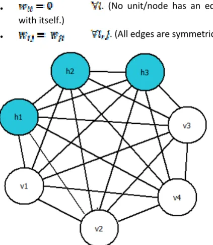
A Boltzmann machine is a neural network which is symmetric with the neural nodes being binary stochastic (randomly determined). In this type of network

, where and are distinct neural nodes. The network consists of two layers viz. hidden and visible. The visible layer consists of visible units/nodes which takes the input as the training set. The total input of node i, is given by,

Where,

  is the stochastic value of the node (on or off)  

  is the bias 

The probability of a node/unit i switching on is given by,

The global energy, in a Boltzmann machine is given by,

where,

  is the weight of the edge between node   and  node   

  are the stochastic value of the node (on or  off)  

  is the bias. 

The edges in the Boltzmann machine network have the following restrictions:

    . (No unit/node has an edge 

with itself.) 

   . (All edges are symmetric.) 

Fig. 2 Boltzmann machine network schematic

Restricted Boltzmann Machine:

Restricted Boltzmann machines are Boltzmann machine with some restrictions. Restricted Boltzmann Machines (RBM) are stochastic bipartite and symmetric networks. RBM consists of two layers viz. hidden and visible. As the network is bipartite, the two layers are disjoint and there are no intra-layer edges in the network. So, visible layer units cannot communicate with other visible layer units and so is the case for hidden layer. RBM weights are randomly initialized and the error in these are removed by backpropogation.

RBM being a bipartite network allows for more effective training algorithms like gradient based contrastive divergence.

Fig. 3 Restricted Boltzmann machine network schematic

The energy of a pair of nodes (v,h) is defined as,

Where,

  is a node from visible layer 

  is  node from hidden layer 

  is bias for visible layer nodes 

  is bias for hidden layer nodes 

  is the weight of the edge between node     and node   

The probability distribution of visible/hidden nodes is given by,

where,

 Z is a partition function that ensures that the sum  of probability distribution is 1. 

  is the energy of a pair of nodes (v,h) 

As RBM networks are bipartite on the two layers (visible and hidden), these layers are conditionally independent of each other. So, we can write:

RBMs with binary units:

RBMs with binary units/nodes is the case where and

. Probabilistic activation probabilities are given by,

III. DEEP BELIEF NETWORK

Deep Belief Networks can be considered as a continuous sequence of layers with each layer made up of Restrictive Boltzmann Machines. Here the network is trained layer by layer in which each layer tries to model the distribution of input using unsupervised learning [2]. Also each layer acts like the hidden layer for the layer before it and as a visible layer for the layer coming after it and thus acts like an input for the next layer. The nodes in each layer are connected to nodes in the next layer forming a complete bipartite graph. Deep belief networks are used for image recognition and generating images. Also if number of layers in the highest layer is small they can perform dimensionality reduction.

The most significant properties of deep belief nets are:

 There is an efficient, layer-by-layer procedure for learning the top-down, generative weights that determine how the variables in one layer depend on the variables in the layer above. 

 Deep belief networks can also be considered as neural networks with more than 3 layers including input and output layers. In deep learning each layer of nodes trains on the distinct outputs received from the previous layer’s output. The further we advance into the network, the more complex the features our nodes can recognize, since they aggregate and recombine features from the previous layer. 

 The biggest advantage of deep learning networks is their ability of discovering structures within raw data which unlabeled and has no structure. Example of such raw data is images, videos, audio recordings. 

However, deep belief networks being suited for unsupervised learning don’t work well with neural networks having stochastic or randomly initialized variables. Hence the deep belief networks need to undergo a phase of pre-learning so that these networks could ‘familiarize’ themselves with the features of the images/data that they are supposed to extract.

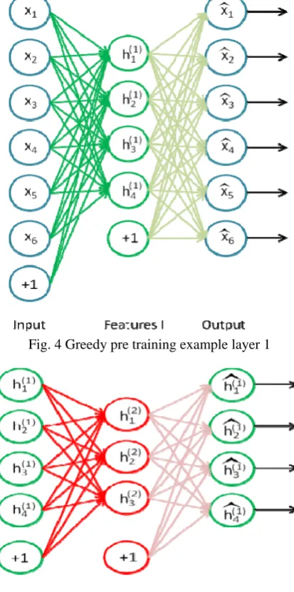
This phase of pre-learning was made faster with a process called as greedy learning. Here in this discussed application, the deep belied network was trained with a open-source dataset of 60,000 images namely ‘MNIST database’.

The basic gist of greedy learning is to train each layer separately such that it will be able to produce its input over multiple back propagations. As a result the variables of each layer get modified in a particular way. These variables are then kept frozen for the entire set.

Once the deep belief networks are trained they can be used to compress any image belonging to the dataset with flexibility in areas of compression ratio, compression time, compression loss.

Fig. 4 Greedy pre training example layer 1

Fig. 5 Greedy pre training example layer 2

Every layer in the deep neural network is going to consist of nodes which are basically computation units similar to brain neurons which fire when a particular input passes through it. These nodes combine data from the input with some weights or coefficients which will either amplify or attenuate the input by multiplying with them. These products are then summed up and these sums are passed through a nodes activation function.

One node might look l

Fig. 7 Representation of a node in deep belief network

Each layer’s output then acts like the input to the following layers. Here the weights of the edges form a weight matrix which is then used to construct the original raw data after it has been compressed by the first deep belief network.

Following is the representation of an entire network.

Fig. 8 Schematic overview of a deep belief network [2].

Each of these layers has random, latent variables. The latent variables generally have binary values which are called as hidden units.

For obtaining these binary latent values from non-binary input following equation is used.

where,

 is the weight of the edge between node and node 

 is the stochastic value of the node (on or off) 



 is the bias 

The stochastic or random values of the weights in each

layer get modified

IV. DEEP AUTOENCODERS

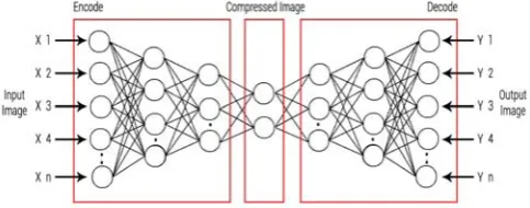
A deep auto encoder encapsulates two; symmetrical deep-belief networks having progressive shallow layers representing the encoding half of the net, and aggressive shallow layers that make up the decoding half. The layers are restricted Boltzmann machines, which build the blocks of deep-belief networks.

Fig. 6 Encoder Decoder pair used for compression

They contain an encoder decoder pair. Here encoders takes raw data (e.g video,image,text) as input value and extracts features from it. These extracted features are used by the decoder as input and restores it back to the raw data as output.

RBMs stacked multiple layers are used to create the encoder and decoder. Training the RBM is associated with feature extraction from the input provided to it. The training process occurs in a layer by layer manner, where a completely trained layer I is fed to layer i+1 as input. This process of training and feeding continues till the stopping criteria are met.

Encoders

We feed 784 (28x28) pixel image to the encoder, the first hidden layer expands the parameters thus expanding the features itself to 1000 nodes, this counterintuitive expansion is mainly done as the sigmoid belief units are in use, which are not as efficient in depicting real value data.

A series of hidden layers having weights 1000,500,250 are used until the net finally produces a 30 bit linearized out depicting the encoded input image. This 30-number vector is the last layer of the first half of the deep auto encoder, the pertaining half, and it is the product of a normal RBM.

Algorithm

Let layer be the matrix of weights controlling functions mapping for layer j to j+1.

Let be the input matrix of layer j. Let function g(z) denote sigmoid of z. For j=0 to max no of layers

Here = raw input images and = reconstructed output image

Decoders

The 30 encoded output numbers are an encoded version of the 28x28 pixel image. The second half of a deep autoencoder deals with decoding these 30 bit numbers back to the 784 pixel format.

The decoding half of a deep autoencoder is a feed-forward net with layers 250, 500 and 1000 nodes wide, respectively. These layers coherently have the same weights as their encoding phase counterparts in the pretraining net, except that the weights are transposed.

Thus the original image is reconstructed back as output in the decoding phase.

V. RESULTS

Thus through the excruciating process of

encoding and decoding with backtracking used to

reduce amount of error generated during encoding,

the final reconstructed image has been generated.

The various phases the image goes through is

depicted below:

Fig. 7 Images at various stages a encoding stage

Thus a 784 by 1000 image finally gets compressed to a 784 by 30.

Lastly the input and output image are compared to show the reconstruction of the compressed image

The figure shows input to output comparison.

Fig. 8 Output and input image comparison

IV.CONCLUSIONS

Thus using deep autoencoders we were able to

compress an image and further reconstruct the

image back from the compressed state. This

mechanism can also be used to classify various

images based on their compressed state and a

two-dimensional graph created can help in

depicting various classes. Thus the important

phenomenon of image compression was

successfully tamed and effectively due to the

promising results of deep autoencoders,

harnessing their power for multi file formats

could lead to its future study and growth. .

REFERENCES

[1] https://www.cs.toronto.edu/~hinton/nipstutorial/nipstut3.pdfJ.

[2] S. Zhang, C. Zhu, J. K. O. Sin, and P. K. T. Mok, “A novel ultrathin

elevated channel low-temperature poly-Si TFT,” IEEE Electron

Device Lett., vol. 20, pp. 569–571, Nov. 1999.

[3] M. Wegmuller, J. P. von der Weid, P. Oberson, and N. Gisin, “High

resolution fiber distributed measurements with coherent OFDR,” in

Proc. ECOC’00, 2000, paper 11.3.4, p. 109.

[4] R. E. Sorace, V. S. Reinhardt, and S. A. Vaughn, “High-speed

digital-to-RF converter,” U.S. Patent 5 668 842, Sept. 16, 1997.

[5] (2002) The IEEE website. [Online]. Available:

http://www.ieee.org/

[6] M. Shell. (2002) IEEEtran homepage on CTAN. [Online]. Available:

http://www.ctan.org/tex-archive/macros/latex/contrib/supported/IEEEtran/

[7] FLEXChip Signal Processor (MC68175/D), Motorola, 1996.

[8] “PDCA12-70 data sheet,” Opto Speed SA, Mezzovico, Switzerland.

[9] A. Karnik, “Performance of TCP congestion control with rate

feedback: TCP/ABR and rate adaptive TCP/IP,” M. Eng. thesis, Indian Institute of Science, Bangalore, India, Jan. 1999.

[10] J. Padhye, V. Firoiu, and D. Towsley, “A stochastic model of TCP

Reno congestion avoidance and control,” Univ. of Massachusetts, Amherst, MA, CMPSCI Tech. Rep. 99-02, 1999.

[11] Wireless LAN Medium Access Control (MAC) and Physical Layer