CMS Computing Resources: Meeting the
demands of the high-luminosity LHC physics
program
David Lange1,*, Kenneth Bloom2 , Tommaso Boccali3,
Oliver Gutsche4, and Eric Vaandering4
1Princeton University, Department of Physics, 08544 Princeton, NJ, USA 2University of Nebraska, Department of Physics, 91944 Lincoln, NE, USA 3INFN Sezione di Pisa, Universita di Pisa, Pisa, ITALY
4Fermilab National Laboratory, 60510, Batavia, Il, USA
Abstract. The high-luminosity program has seen numerous extrapolations of its needed computing resources that each indicate the need for substantial changes if the desired HL-LHC physics program is to be supported within the current level of computing resource budgets. Drivers include large increases in event complexity (leading to increased processing time and analysis data size) and trigger rates needed (5-10 fold increases) for the HL-LHC program. The CMS experiment has recently undertaken an effort to merge the ideas behind short-term and long-term resource models in order to make easier and more reliable extrapolations to future needs. Near term computing resource estimation requirements depend on numerous parameters: LHC uptime and beam intensities; detector and online trigger performance; software performance; analysis data requirements; data access, management, and retention policies; site characteristics; and network performance. Longer term modeling is affected by the same characteristics, but with much larger uncertainties that must be considered to understand the most interesting handles for increasing the "physics per computing dollar" of the HL-LHC. In this presentation, we discuss the current status of long term modeling of the CMS computing resource needs for HL-LHC with emphasis on techniques for extrapolations, uncertainty quantification, and model results. We illustrate potential ways that high-luminosity CMS could accomplish its desired physics program within today's computing budgets.
1 Introduction
Given the scale, and thus cost of, the LHC computing requirements [1], modeling efforts aimed at projecting experiment resource needs started even before data taking in Run 1 of the LHC [2]. The goal of these models is to capture sufficient detail of the experiment’s physics requirements, LHC performance expectations and experiment’s tiered computing model to accurately project the level of CPU, disk and tape resources needed
from each computing tier supporting the experiment. Results from these models provide input to external reviews, including both short-term estimates of needs and long-term projections for the high-luminosity LHC (HL-LHC) program. In particular, the resource requests are made by LHC experiments and reviewed at six month intervals. To match budget cycles, these reviews assess the computing needs two years ahead. For example, in spring of 2018, these reviews assess requests for 2020.
Internally, modeling tools understand the implications of evolutions to computing models. In particular, good models will help to identify critical components that drive resource needs, and demonstrate impact of physics choices and R&D activities.
2 Model evolution
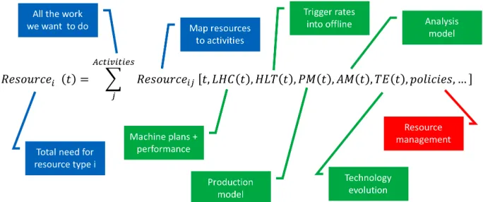
Initially simple models have now become complex to meet growing demands for accuracy, fidelity and timescales. Figure 1 illustrates the current approach by the CMS experiment [3] for both short-term and long-term projections.
Figure 1: High-level view of how the CMS resource models build up total resource needs from the underlying inputs.
Examples of parameters needed as input include:
1. What workflows will be run by the experiment, where they will run, and when they will run. These details can help define the overall resource need, and also periods of peak resource need that might need to be considered as resource planning is done.
2. Evolution of experiment workflows, data tiers, analysis requirements, and other attributes of how the experiment anticipates running its infrastructure. Research and development is always on-going. Once deployed, results of this R&D impact may have a big impact on the computing resource needs of an experiment. For example, a small data tier becoming more widely used for analysis will reduce the overall disk need.
3. Evolution with instantaneous luminosity, in particular the average number of pileup events expected. Time to process each event is quite sensitive to the event complexity, most often characterized by the average pileup. The processing time for both data and Monte Carlo simulation samples should be modeled accordingly. 4. Evolution with integrated luminosity, in particular the total luminosity impacts the
amount of Monte Carlo simulation required by analysts. Annual luminosity estimates are available from the LHC through the first years of HL-LHC [4].
5. Impact of LHC reliability, in particular the number of data taking seconds per year impacts the total event sample collected. While trigger output rates are typically a function of luminosity, they also have a component that is more constant. For example, CMS [5] and ATLAS [6] quote average rates of 1 kHz during Run 2 as input to modeling results.
6. Expected analysis user behaviour, such as peaks of activity for conferences and the overall level of analysis processing expected. Analysis processing is an important, but difficult to model, aspect of computing resource needs. The use of monitoring information is important for deciding how to include (e.g., which parameters) analysis into a model. In CMS we consider how many times, on average, events are read during a month, as well as how the data set used by most analysts will evolve with time. For example, each change of center-of-mass energy in data taking effectively resets the analysis data set of most interest (once data from that new energy is completely reconstructed and calibrated).
7. Evolving balance of commissioning needs, production needs and analysis needs. Planning of computing resources often neglects special needs such as those for detector commissioning or for preparing for new processing activities. These needs can be large in the case that samples of raw detector data or other large data sets are needed (which would otherwise be on tape).
8. Impact of site infrastructure needs. Like the experiment software stack, site infrastructure continues to evolve. Models need to be capable of including new attributes as they become relevant for planning purposes. Topical examples include network requirements, tape recall rates, or on the long term the availability of accelerators.
9. Use of dynamic and heterogeneous resources, such as when the high-level trigger farm is likely to be available for offline workflows. Dynamic resources can reduce the overall need, in particular for CPU, as they can be used in periods of peak need, or alternatively to complete processing tasks more quickly than they otherwise would be. The challenge is to determine the extent to which these resources can be included in the computing resource need planning process. Often their availability is highly uncertain when projections are made. For example, this can be due to the process of making allocation requests. Conversely, the availability of a high-level trigger farm for processing is more predictable, as it is essentially correlated with data taking periods.
10. Policies that ensure efficient resource usage, such as data management policies. As the pressure on resources increases, more and more complex systems for the agile management of storage resources are important. It is difficult to build first-principles models of how policies will impact resource usage. Conversely policies can have a large effect on resource requirements, so they must be included in any model.
3 New computing resource model for CMS
As CMS started to look towards estimates of Run 3 and HL-LHC computing resource needs, we decided that a new implementation of the model itself is needed in order to naturally increase the fidelity of the model to match the evolutions towards these runs. CMS has chosen a programmatic solution rather than a spreadsheet driven solution for modeling needs going forward. In our view, advantages of this approach include:
from each computing tier supporting the experiment. Results from these models provide input to external reviews, including both short-term estimates of needs and long-term projections for the high-luminosity LHC (HL-LHC) program. In particular, the resource requests are made by LHC experiments and reviewed at six month intervals. To match budget cycles, these reviews assess the computing needs two years ahead. For example, in spring of 2018, these reviews assess requests for 2020.
Internally, modeling tools understand the implications of evolutions to computing models. In particular, good models will help to identify critical components that drive resource needs, and demonstrate impact of physics choices and R&D activities.
2 Model evolution
Initially simple models have now become complex to meet growing demands for accuracy, fidelity and timescales. Figure 1 illustrates the current approach by the CMS experiment [3] for both short-term and long-term projections.
Figure 1: High-level view of how the CMS resource models build up total resource needs from the underlying inputs.
Examples of parameters needed as input include:
1. What workflows will be run by the experiment, where they will run, and when they will run. These details can help define the overall resource need, and also periods of peak resource need that might need to be considered as resource planning is done.
2. Evolution of experiment workflows, data tiers, analysis requirements, and other attributes of how the experiment anticipates running its infrastructure. Research and development is always on-going. Once deployed, results of this R&D impact may have a big impact on the computing resource needs of an experiment. For example, a small data tier becoming more widely used for analysis will reduce the overall disk need.
3. Evolution with instantaneous luminosity, in particular the average number of pileup events expected. Time to process each event is quite sensitive to the event complexity, most often characterized by the average pileup. The processing time for both data and Monte Carlo simulation samples should be modeled accordingly. 4. Evolution with integrated luminosity, in particular the total luminosity impacts the
amount of Monte Carlo simulation required by analysts. Annual luminosity estimates are available from the LHC through the first years of HL-LHC [4].
5. Impact of LHC reliability, in particular the number of data taking seconds per year impacts the total event sample collected. While trigger output rates are typically a function of luminosity, they also have a component that is more constant. For example, CMS [5] and ATLAS [6] quote average rates of 1 kHz during Run 2 as input to modeling results.
6. Expected analysis user behaviour, such as peaks of activity for conferences and the overall level of analysis processing expected. Analysis processing is an important, but difficult to model, aspect of computing resource needs. The use of monitoring information is important for deciding how to include (e.g., which parameters) analysis into a model. In CMS we consider how many times, on average, events are read during a month, as well as how the data set used by most analysts will evolve with time. For example, each change of center-of-mass energy in data taking effectively resets the analysis data set of most interest (once data from that new energy is completely reconstructed and calibrated).
7. Evolving balance of commissioning needs, production needs and analysis needs. Planning of computing resources often neglects special needs such as those for detector commissioning or for preparing for new processing activities. These needs can be large in the case that samples of raw detector data or other large data sets are needed (which would otherwise be on tape).
8. Impact of site infrastructure needs. Like the experiment software stack, site infrastructure continues to evolve. Models need to be capable of including new attributes as they become relevant for planning purposes. Topical examples include network requirements, tape recall rates, or on the long term the availability of accelerators.
9. Use of dynamic and heterogeneous resources, such as when the high-level trigger farm is likely to be available for offline workflows. Dynamic resources can reduce the overall need, in particular for CPU, as they can be used in periods of peak need, or alternatively to complete processing tasks more quickly than they otherwise would be. The challenge is to determine the extent to which these resources can be included in the computing resource need planning process. Often their availability is highly uncertain when projections are made. For example, this can be due to the process of making allocation requests. Conversely, the availability of a high-level trigger farm for processing is more predictable, as it is essentially correlated with data taking periods.
10. Policies that ensure efficient resource usage, such as data management policies. As the pressure on resources increases, more and more complex systems for the agile management of storage resources are important. It is difficult to build first-principles models of how policies will impact resource usage. Conversely policies can have a large effect on resource requirements, so they must be included in any model.
3 New computing resource model for CMS
As CMS started to look towards estimates of Run 3 and HL-LHC computing resource needs, we decided that a new implementation of the model itself is needed in order to naturally increase the fidelity of the model to match the evolutions towards these runs. CMS has chosen a programmatic solution rather than a spreadsheet driven solution for modeling needs going forward. In our view, advantages of this approach include:
2.Clarity of input parameters: Various human readable formats can be easily used to describe and document each input parameter.
3.Not monolithic: Programmatic approaches are easier to design for enabling a wide variety of model analysis, such as parameter trade-off studies.
4.Version control and change tracking: Code for the model itself, as well as input data evolution and model results can easily be tracked and shared
5.Unit testing: Model components can be more easily tested to ensure robustness as the model evolves and becomes more complex.
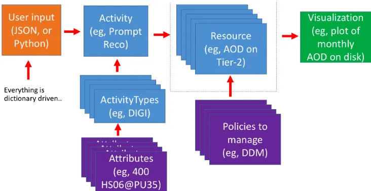
Figure 2 illustrates the basic building blocks of our implementation.
Figure 2: Resource estimate model building blocks
In short the primary concepts of the model include:
1. Input: Specifications of each model component are user driven. The current implementation supports a JSON interface and a Python interface for defining model components. These may be mixed and matched. The primary reason for a Python interface is to make it easy to define repetitive model components without excessive duplication. For example, a processing activity performed each year is most easily defined in a loop.
2. Activities: Activities are the model component that defines a unit of work to be done by the experiment’s computing system. For example, “prompt reconstruction in 2018” is an Activity. Activities are defined by start and end times, data taking periods that they should include (e.g., 2018), a model for the number of events to be produced or processed, the number of times each event should be produced or processed (e.g., for analysis user activity) and a list of “ActivityTypes” included.
3. ActivityTypes: ActivityTypes are the model component representing a specific workflow, for example digitization or event reconstruction. These most naturally correspond to a single application run by the experiment. ActivityTypes are defined by the list of Attributes that are required, and the fraction of events that are expected to have each Attribute. For example, the prompt reconstruction activity might have an attribute for CPU required as well as each type of output data, each of which ends up on different disk or tape systems.
4. Attributes: Attributes define the properties of ActivityTypes, and are defined by a resource type (e.g., Tier-1 disk) and resource purpose (e.g., storage of the AOD data tier). Attributes define the model for how much of a resource is needed (per event) as a function of relevant parameters. An example is that the AOD data tier size per event typically depends on pileup (the number of simultaneous proton-proton interactions in a LHC bunch crossing seen by CMS). In this case, the Attribute could be defined as a lookup table that is a function of the average pileup in a data taking period, or as a polynomial function.
5. ResourceTypes: Each relevant computing infrastructure component to be monitored corresponds to a ResourceType. For example, Tier-1 disk or Tier-0 CPU are ResourceTypes for the CMS model. ResoureTypes include parameters inherent to the computing resource, such as a nominal efficiently metric. For example, this may represent the nominal CPU efficiency, or maximum percentage filled for disk.
6. ResourcePurposes: Each relevant consumer of any ResourceType is denoted as a ResourcePurpose. Examples include the CPU needed for reconstruction, the storage needed for RAW data.
7. Resources: Resources define the amount of each computing infrastructure component needed for each purpose. Resources include a ResourceType, a ResourcePurpose, and an amount (e.g., HS06/event).
8. Policies: The model does not yet include a generic class for capturing resource management policies. The model does include an implementation for a data management policy. The number of replicas of each ResourcePurpose on each ResourceType evolves according to a time-dependent model. The model may be different depending on if the data corresponds to the last ResourcePurpose that was processed for a given data taking era. This last feature is meant to capture reprocessings, when the last reprocessing is of more interest than the previous ones.
9. Visualization tools: The model includes both plotting and tabular visualization tools. Both types of tools bin data according to the time period (e.g., annually or monthly), and grouped or split by ResourcePurpose or ResourceType. The plots to be included are user defined. The plotting toolkit is backed by the matplotlib [7] package.
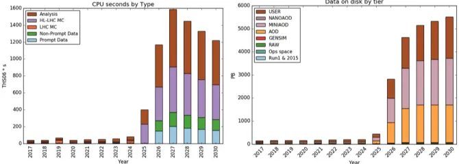
Example results are shown in Figure 3, where the estimated evolution in CMS CPU and disk requirements are shown.
Figure 3: Current estimates for CMS CPU and disk needs through the initial years of the HL-LHC
2.Clarity of input parameters: Various human readable formats can be easily used to describe and document each input parameter.
3.Not monolithic: Programmatic approaches are easier to design for enabling a wide variety of model analysis, such as parameter trade-off studies.
4.Version control and change tracking: Code for the model itself, as well as input data evolution and model results can easily be tracked and shared
5.Unit testing: Model components can be more easily tested to ensure robustness as the model evolves and becomes more complex.
Figure 2 illustrates the basic building blocks of our implementation.
Figure 2: Resource estimate model building blocks
In short the primary concepts of the model include:
1. Input: Specifications of each model component are user driven. The current implementation supports a JSON interface and a Python interface for defining model components. These may be mixed and matched. The primary reason for a Python interface is to make it easy to define repetitive model components without excessive duplication. For example, a processing activity performed each year is most easily defined in a loop.
2. Activities: Activities are the model component that defines a unit of work to be done by the experiment’s computing system. For example, “prompt reconstruction in 2018” is an Activity. Activities are defined by start and end times, data taking periods that they should include (e.g., 2018), a model for the number of events to be produced or processed, the number of times each event should be produced or processed (e.g., for analysis user activity) and a list of “ActivityTypes” included.
3. ActivityTypes: ActivityTypes are the model component representing a specific workflow, for example digitization or event reconstruction. These most naturally correspond to a single application run by the experiment. ActivityTypes are defined by the list of Attributes that are required, and the fraction of events that are expected to have each Attribute. For example, the prompt reconstruction activity might have an attribute for CPU required as well as each type of output data, each of which ends up on different disk or tape systems.
4. Attributes: Attributes define the properties of ActivityTypes, and are defined by a resource type (e.g., Tier-1 disk) and resource purpose (e.g., storage of the AOD data tier). Attributes define the model for how much of a resource is needed (per event) as a function of relevant parameters. An example is that the AOD data tier size per event typically depends on pileup (the number of simultaneous proton-proton interactions in a LHC bunch crossing seen by CMS). In this case, the Attribute could be defined as a lookup table that is a function of the average pileup in a data taking period, or as a polynomial function.
5. ResourceTypes: Each relevant computing infrastructure component to be monitored corresponds to a ResourceType. For example, Tier-1 disk or Tier-0 CPU are ResourceTypes for the CMS model. ResoureTypes include parameters inherent to the computing resource, such as a nominal efficiently metric. For example, this may represent the nominal CPU efficiency, or maximum percentage filled for disk.
6. ResourcePurposes: Each relevant consumer of any ResourceType is denoted as a ResourcePurpose. Examples include the CPU needed for reconstruction, the storage needed for RAW data.
7. Resources: Resources define the amount of each computing infrastructure component needed for each purpose. Resources include a ResourceType, a ResourcePurpose, and an amount (e.g., HS06/event).
8. Policies: The model does not yet include a generic class for capturing resource management policies. The model does include an implementation for a data management policy. The number of replicas of each ResourcePurpose on each ResourceType evolves according to a time-dependent model. The model may be different depending on if the data corresponds to the last ResourcePurpose that was processed for a given data taking era. This last feature is meant to capture reprocessings, when the last reprocessing is of more interest than the previous ones.
9. Visualization tools: The model includes both plotting and tabular visualization tools. Both types of tools bin data according to the time period (e.g., annually or monthly), and grouped or split by ResourcePurpose or ResourceType. The plots to be included are user defined. The plotting toolkit is backed by the matplotlib [7] package.
Example results are shown in Figure 3, where the estimated evolution in CMS CPU and disk requirements are shown.
Figure 3: Current estimates for CMS CPU and disk needs through the initial years of the HL-LHC
4 Model trade-off studies
An important attribute of any model is the ability to not only produce coherent and consistent results, but to facilitate parameter sensitivity studies. Being able to identify the most critical parameters is especially important as HEP looks to identify the most important areas for research and development in software and computing for HL-LHC.
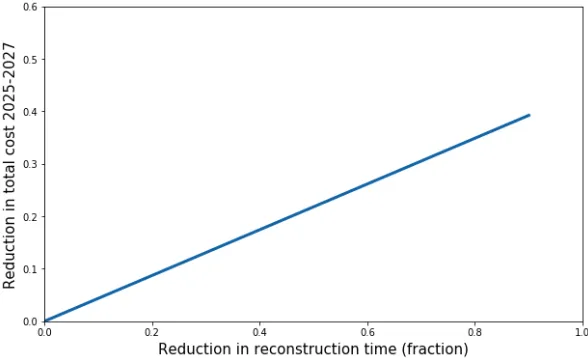
An example of this sort of analysis is illustrated in Figures 4 and 5, where we show code and corresponding visualization for how the cost metric might depend on the time needed for reconstructing each event in the HL-LHC era. Estimating cost is itself a potentially complex undertaking. We built a simplistic model based on current equipment costs, its evolution and lifetime at U.S. Tier-2s in CMS to provide enough fidelity for relative cost comparisons (absolute comparisons being more complex). From this model, we defined a “cost metric” as the corresponding cost of the start-up phase of HL-LHC where the computing costs are expected to be highest.
Given this cost metric, we can simply change the reconstruction time in the model, rerun and tabulate the cost as a function of reconstruction time, as shown in Figure 5.
Figure 4: Pseudo-code example of how the event reconstruction time can be varied to perform a tradeoff study.
Figure 5: Example results illustrating the fractional cost savings as a function of the fractional reduction in CPU time needed to reconstruct each event offline.
5 Conclusion
We have presented an initial look at a new approach to implementing a computing resource model capable of making Run 2, Run 3 as well as HL-LHC resource projections. While developed in the context of CMS, the design and implementation have focused on user-input driven design which should enable others to use this software once released. We expect to release an initial version by the end of 2018 or early 2019.
References
1. I. Bird, et. al., CERN-LHCC-2014-014, (2014). 2. L. Evans and P. Bryant, JINST 3 S08001 (2008). 3. CMS Collaboration, JINST 03 S08004 (2008).
4. LHC long term schedule, http://lhc-commissioning.web.cern.ch/lhc-commissioning/schedule/LHC-long-term.htm (visited December 2018).
4 Model trade-off studies
An important attribute of any model is the ability to not only produce coherent and consistent results, but to facilitate parameter sensitivity studies. Being able to identify the most critical parameters is especially important as HEP looks to identify the most important areas for research and development in software and computing for HL-LHC.
An example of this sort of analysis is illustrated in Figures 4 and 5, where we show code and corresponding visualization for how the cost metric might depend on the time needed for reconstructing each event in the HL-LHC era. Estimating cost is itself a potentially complex undertaking. We built a simplistic model based on current equipment costs, its evolution and lifetime at U.S. Tier-2s in CMS to provide enough fidelity for relative cost comparisons (absolute comparisons being more complex). From this model, we defined a “cost metric” as the corresponding cost of the start-up phase of HL-LHC where the computing costs are expected to be highest.
Given this cost metric, we can simply change the reconstruction time in the model, rerun and tabulate the cost as a function of reconstruction time, as shown in Figure 5.
Figure 4: Pseudo-code example of how the event reconstruction time can be varied to perform a tradeoff study.
Figure 5: Example results illustrating the fractional cost savings as a function of the fractional reduction in CPU time needed to reconstruct each event offline.
5 Conclusion
We have presented an initial look at a new approach to implementing a computing resource model capable of making Run 2, Run 3 as well as HL-LHC resource projections. While developed in the context of CMS, the design and implementation have focused on user-input driven design which should enable others to use this software once released. We expect to release an initial version by the end of 2018 or early 2019.
References
1. I. Bird, et. al., CERN-LHCC-2014-014, (2014). 2. L. Evans and P. Bryant, JINST 3 S08001 (2008). 3. CMS Collaboration, JINST 03 S08004 (2008).
4. LHC long term schedule, http://lhc-commissioning.web.cern.ch/lhc-commissioning/schedule/LHC-long-term.htm (visited December 2018).