HIVEC: A Hierarchical Approach for Vector
Representation Learning of Graphs
Ayushi Patel
1,∗, Ramakrishna R M
1,∗, Mausam Jain
2,†, Krishnakant Singh
2,†,
Naveen Sivadasan
3, Vineeth N Balasubramanian
21Department of Engineering Science, Indian Institute of Technology Hyderabad, India
2Department of Computer Science, Indian Institute of Technology Hyderabad, India
3Tata Consultancy Services - Innovation Labs, Hyderabad, India
1{es14btech11003, es14btech11015}@iith.ac.in,
2{cs15mtech11009, cs15mtech11007, vineethnb}@iith.ac.in,
3
Abstract—This paper presents a new method : HIVEC to learn latent vector representations of graphs in a manner that captures the semantic dependencies of sub-structures. The representations can then be used in machine learning algorithms for tasks such as graph classification, clustering etcetera. The method proposed is unsupervised and uses the information of co-occurrence of sub-structures. It introduces a notion of hierarchical embeddings that allows us to avoid repetitive learning of sub-structures for every new graph. As an alternative to deep learning methods, the edit distance similarity between sub-structures is also used to learn vector representations. We compare the performance of these methods against previous work.
Keywords—Deep learning, graph kernels, unsupervised learn-ing
I. INTRODUCTION
Today, graphs are common entities that are used to repre-sent information and data from various real-world scenarios. These could be the relationships between people in social networking, interaction of atoms and molecules in study of chemicals or the protein-protein interaction in the study and discovery of drugs. Graphs allow to explore properties of these real-world objects and thus facilitate to make comparison between them. For instance, in a social network, the essence of communities is well highlighted when the network is represented as a graph, where people are vertices and their interactions (messages, tags, pokes etc.) are edges between those vertices. Similarly, in the field of compiler construction, a DAG (directed acyclic graph) is used to represent the flow of execution of instructions and explore the dependencies and redundancies within them. The state-of-the-art machine learning techniques aim to learn features from these graphs and discover interesting relationships within them which can be between any two vertices or any two sub-graphs in the original graph. Community detection, recommendation systems and community-similarity score between any two groups in social network are some applications of machine learning on graphs. For a million sized graph, it becomes difficult for these tasks to process graphs in the for of their adjacency matrices. Thus, there is the need to learn latent representations of graphs and the components (vertices and sub-graphs) within them.
There have been plenty of research done in this domain. The pioneer work in this area is DeepWalk by Perrozi et.al. [1] in their work on learning latent vector representations of vertices in graphs. Their work is motivated by the advancements in language modeling techniques in natural language processing. They treat random walks in a graph as sentences in NLP and use skipgram model introduced in [2] to find vector representations of vertices in graph. DeepWalk achieved good latent vectors of vertices which can be used to study various important properties of the graph. Followed by this work, Tang et.al. [3] in their work proposed a method to get embeddings of nodes in a graph by considering two-level neighborhood of a vertex where as DeepWalk considers only the imme-diate neighbours of a vertex. They also propose an edge-sampling algorithm to optimize the objective function and achieve considerably good results. Another work in this area is proposed in [4] where again authors aim to find latent vector representations of vertices in graph by a slightly modified approach as in previous two cited works. All these works focus on representing vertices as latent vectors which led the research to move to getting representations of sub-structures in graph. Most famous work in this area is Deep Graph Kernels [5] by Yanardag and Vishwanathan. In this authors propose a method to find vector embeddings of subgraphs by mixing classical kernels and the skipgram model. Following this work, Narayan and co-authors proposed another technique in [6] which is a slight modification of [5] and achieve comparable results in getting rich embeddings of sub-structures in graph. Both these sub-structure learning techniques depend upon the input graph to learn representations of sub-structures and use direct frequency counting vectors to get the kernel matrix which is not the case in our method. HIVEC learns the embeddings of sub-structures (here graphlets) beforehand irrespective of what an how the input graph is. This saves the tasks of training skipgram model everytime a new graph comes Also, this method introduces a novel approach called
hierarchical embeddingto get the frequency vector for kernel matrix computation. The key contributions of this paper are
• Graphlet embeddings are learned irrespective of the input
graph considering the fact that every graph consists of basic sub-structures (graphlets) and almost identical neighborhood environment. This prevents the time taken to learn graphlet embeddings for every new graph.
• We propose ahierarchicalapproach to learn the embeddings of graph by learning a kernel matrix which respects the sparse and dense topology of any given graph.
Graph Kernels: Graph Kernels are one of the popular
and widely adopted approaches to measure similarities among graphs. A Graph kernel measures the similarity between a pair of graphs by recursively decomposing them into atomic sub-structures (e.g., walk [7], shortest paths [8], graphlets [9], [10] etc.) and defining a similarity function over the sub-structures (e.g., number of common sub-sub-structures across both graphs).This makes the kernel function correspond to an inner product over sub-structures. Formally, for a given graphG, let
Φ(G) denote a vector which contains counts of atomic sub-structures, and h.,.iH denote a dot product. Then, the kernel between two graphs GandG'is given by
K(G, G0) =hΦ(G),Φ(G0)iH (1)
This kernel matrix K representing pair-wise similarity of graphs in the dataset (using equation (1)) could be used in conjunction with kernel classifiers (like Support Vector Machine (SVM)) and relational data clustering algorithms to perform graph classification and clustering tasks, respectively.
II. RELATEDWORK
There have been plenty of methods proposed in the space of learning latent vector representations for nodes and sub-graphs. Each work roughly varies in the way it defines and generates the corpus for deep model learning. We are going to discuss them briefly in this section.
• DeepWalk: Perozzi et.al. [1] in their work, proposed a
method to find representations of vertices in graphs. Their method considers only the topology of the network to find embeddings of vertices. They make use of Deep Learning techniques, defined in natural language processing, for the graphs. They treat sentences in NLP equal to random walks in graphs. In this way, by forming sequences of vertices, by performing some fixed number of random walks for some fixed number of times, starting at each vertex in the graph, they give these input to word2vec skipgram model (Figure 2) and learn embeddings of vertices. They show that representing these vector embeddings in space, one can get sense of communities in the graph and also the distance between any two vertices in the graph. Following this work, there has been many other proposed methods for learning embeddings of vertices [4].
• Deep Graph Kernels: A major short coming of graph
kernels defined using equation (1), is addressed in paper by, Yanardag and Vishwanathan [5], by an alternative formulation of kernels in a manner that captures the similarity between substructures as in equation (2) which is not accounted for in vanilla graph kernels. The paper takes inspiration from representation learning methods like the
work of Mikolov et al. [1], traditionally used in language modeling, where representations of words is learnt using a deep learning method from the context where they occur in a sentence. The notion of context is introduced for different sub-structures. With this approach, they trained deep learning variants of popular graph kernels such as graphlet, WL and shortest path kernels, out of which Deep WL kernels achieved state of the art performance on several datasets.
• Subgraph2Vec: Narayanan et.al. [6] proposed a method in
their work, to learn graph representations using a similar approach as in [5] except that they generate the corpus for word2vec model differently. For each vertex vi, they find a subgraph of some degree d and find its radial context in which they find sub-graphs of degrees d-1, d
andd+1 starting from adjacent vertices ofvi. In this way, the context is formed and skipgram model is trained to get representations of sub-graphs.
III. METHODOLOGY
In contrast to vocabulary generation methods discussed in [5], [6], we present a novel and reliable approach to generate the same for language modelling technique, which improves over previous methods. The main contribution of this paper is introduction to hierarchical embedding which takes into account the sparsity and density in the topology of the graph to compute the kernel matrix. We then discuss the three methods for learning vector embeddings of sub-structures which are then used to find embedding of graphs under consideration.
A. Approach
In [5], they propose a modification in the graphlet based graph kernel. Graphlet kernel gives an explicit embedding φ(G) in n-dimensional space where n corresponds to the frequency count of the corresponding graphlet in G as an induced subgraph. As graphlet size increases, n increases exponentially and the components have correlations. Hence they propose a kernel kdefined as:
k(G, G0) =φ(G)TMφ(G0) (2)
where,Mis an×npositive semi-definite matrix representing the relation between the graphlets.
In our approach, we first obtain a set ofnsub-structures each withd-dimensional vector embedding, using word2vec to get the matrixRn×d. This is then extended to get representations
of larger graph G, where we follow graphlet based approach to findφ(G), then-dimensional frequency vector with respect to all thensub-structures. Now, letMn×n be the dot product matrix between all pairs of sub-structures with respect to their
d-dimensional word2vec embeddings. Using matrix factoriza-tion, matrixM can be written as,
M=R×RT (3)
So, using equation (3), (2) can be written as,
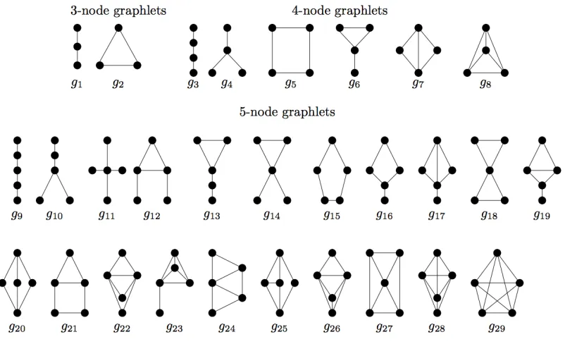
Fig. 1. All graphlets of size 3,4,5
Fig. 2. Dependency of sub-structures giving rise to the notion ofedit-distance
relationship between them.
Hence, from equation (4) we can define a new embedding for graph Gas
φ0(G) =RTφ(G) (5)
Above equation gives a d-dimensional vector representation of any graph G derived using sub-structures contained in it. This vector is expected to have semantic information about the overall topological structure of G. Now, equation (4) can be rewritten as, using equation (5),
k(G, G0) =φ0(G)Tφ0(G0) (6)
So, from above equation, we can get a similarity measure between any two arbitrary graphs using their vector representations.
The problem with above approach is that when the size of the graph G becomes large we need to have counts of larger sub-structures and find their embeddings using word2vec. This is not scalable because everytime when a
new graph is considered, number of graphlets to be counted will change and need to be trained again. Also, training for a large vocabulary all over again is not a good approach for real time applications. To overcome this problem, we define a concept of hierarchical embedding which avoids the need of learning embeddings again as new graph is encountered.
Hierarchical Embedding for larger graphs: The
em-bedding in equation (5) can be extended to a hierarchical embedding for a graphGas explained next.
Let us define a setS1denoting graphlets each of size sayt. Let
|S1| = n1. Also, lets consider a hierarchy of k such families
as S1, S2, . . . , Sk. The graphlets in the set S2 would each then be of size t+1 (though this is not a strict requirement, the hierarchy could be arbitrarily distant from each other). So, for any j ∈ {1, 2, . . . , k}, |Sj| = nj. Now, let us consider Φj(G) for j ∈ {1, 2, . . . , k}, denote the graphlet frequency vector corresponding to the graph G where the graphlets are from set Sj. Hence, Φj(G) is a nj-dimensional vector. Now,
let φ'(G) be the final expected d-dimensional embedding (as in equation (5)). This gives φ'(s11),φ'(s12), . . . ,φ'(n1) denote the embeddings for level-1 graphlets, which are learned using word2vec and their -neighbourhoods, belonging to the set S1. From all these, the level-1 embedding of a graph G can be written as
φ0(G) = Φ1(G)×D1 (7)
whereD1 is a matrix with dimensions n1 ×d denoting each
row corresponding to one ofφ'(s11),φ'(s12), . . . ,φ'(n1). Extending the above equation, the level-2 embedding for the graphGcan be written as
Fig. 3. Skipgram Model
where D2 is a matrix with dimensions n2 × d denoting
each row corresponding to one of φ'(s21),φ'(s22), . . . ,φ'(n2), graphlets belonging to the setS2. From previous explanations, for every sj ∈ S2, its embeddingφ'(sj) can be written as
φ0(sj) = Φ1(sj)×D1 (9)
Thus, we can replace matrix D2 and rewrite the level-2 embedding of graph Gin equation (8) as
φ0(G) = Φ2(G)×F1×D1 (10)
whereF1is a matrix with dimensionsn2×n1where each row corresponds to one ofΦ1(s1), . . . ,Φ1(sn2), for all graphlets in setS2. Generalizing the above equation, a level-kembedding of graphGcan be defined as
φ0(G) = Φk(G)×Fk-1×Fk-2× · · · ×F1×D1 (11)
where Φk(G) is the frequency vector corresponding to graph
Gwith respect to level-kgraphlets, belonging to set Sk.
Let us assumegk(G), an
k-dimensional vector where nk is the number of level-kgraphlets in setSk. This vector is defined as
weighted frequency vector in comparison to naive frequency vector Φk(G) as explained below.
Interpretation of weighted frequency vector: Vectorgk(G)
can be interpreted as a weighted graphlet frequency vector for graph G with respect to level-1 graphlets, also known as basic graphlets, of set S1 in the way explained below. Let us
consider a specific occurrence of basic graphletsi in graphG.
Now, we count the different connected induced sub-graphs in
G each of size kand containing this graphlet si. Summation
of these counts, for all occurences of basic graphlets si in
G, corresponds to the ith component of vectorgk(G). Having
this sense,gkcan be said to be a weighted graphlet frequency
vector. The above reasoning can be argued in a way that if two occurrences of a graphlet si are such that one is in a dense
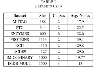
TABLE I
DATASETS USED
Dataset Size Classes Avg. Nodes
MUTAG 188 2 17.9
PTC 344 2 25.5
ENZYMES 600 6 32.6 PROTEINS 1113 2 39.1 NCI1 4110 2 29.8 NCI109 4127 2 29.6
IMDB-BINARY 1000 2 19.77 IMDB-MULTI 1500 3 13
region and the other is in the sparse region of graph G and so the one in dense regions gets more weight than the other one in sparse region. This is because there are many morek -sized sub-graphs possible in the dense region and having this graphlet occurrence as compared to the sparse region. This is better frequency vector representation as compare to the naive
Φ1(G) which treats all occurrences of graphlets of same type uniformly. Equation (11) now can be rewritten as:
φ0(G) =gk(G)×D
1 (12)
Approximation of weighted frequency vector: Given a
graph G, for each vertex vi ∈ V, we perform a breadth first search starting atvi. In this way, we consider neighbourhoods of each vertex upto some depthp. Let, this induced subgraph be denoted as Gu. Now, letfu denote the graphlet frequency vector forGu with respect to level-kgraphletsSk.
fu= Φk(Gu) (13)
Let,fi,udenotes the frequency vector corresponding to the BFS done with starting vertexvi. Then, approximatinggk(G) as
ˆ
gk(G) =X i∈V
fi,u (14)
The reason this approximation is good is that any specific occurrence of a graphlet in Gwould be scaled by its neigh-borhood. A given graphlet in a dense region of the graph will be counted many more times compared to an occurrence in a sparse region. This is because, in the dense region, the graphlet would be part of the BFS neighborhoods of lot more vertices than in the sparser one. Thus, from equation (11), we get final embedding of the graphGas
φ0(G) = ˆgk(G)×D1 (15)
IV. LEARNINGVECTOREMBEDDINGS
A. Edit-Distance Similarity between Sub-structures
Edit-distance between any two graphlets is defined as the total number of edges that are to removed/added to make both the two graphlets equal. For instance, in graphlet kernels, one can derive edit-distance relationship to encode how similar one graphlet is to another (see Figure 2). Given a graphlet
Gi of size k and a graphletGj of size k + 1, let us build an
undirected graph Q based on edit-distances of graphlets, by adding an undirected edge fromGitoGj if and only ifGican
be obtained from Gj by adding an edge to it (or viceversa).
Given such an undirected graph Q, one can simply compute the shortest-path distance between every pair of graphlets in the vocabulary. As we only consider connected graphlets of size 3 ≤k ≤5, this method is not computationally costly. We, thus get a twenty nine dimensional square matrix D where each element denotes edit-distance similarity measure between any two graphlets. We then perform singular value decomposition of matrixDas shown below.
D=uΣv> (16)
Using top fifteen eigenvalues from diagonal matrix Σ, we get latent representations for all the sub-structures.
B. Language Modelling - Skipgram Model
In this approach, we learn latent vectors using recently introduced language modeling and deep learning techniques. We first review the related background in language modeling, and then transform the ideas to learn representations of sub-structures.
1) Neural language models: Traditional language models estimate the likelihood of a sequence of words appearing in a corpus. Given a sequence of training words {w1 , w2 , . . . ,
wT}, n-gram based language models aims to maximize the
following probability
Pr(wt|w1, w2, . . . , wt-1) (17)
The above probability estimates the likelihood of observingwt
givenn previous words observed so far.
Recent work in language modeling focused on distributed vector representation of words, also referred as word embed-dings. These neural language models improve classicn-gram language models by using continuous vector representations for words. Unlike traditionaln-gram models, neural language models take advantage of the notion of context where a context is defined as a fixed number of preceding words. In practice, the objective of word embedding models is to maximize the following log-likelihood
T
X
t=1
log Pr(wt|wt-n+1, w2, . . . , wt-1) (18)
wherewt-n+1, . . . ,wt-1is the context ofwt. We will now discuss a method that approximates the above equation which we utilize in our framework, namely Skipgram model [11].
2) Skip-gram Model: The Skip-gram model maximizes co-occurrence probability among the words that appear within a given window. In other words, instead of predicting the current word based on surrounding words, the main objective of the Skip-gram is to predict the surrounding words given the current word (see Figure 3). More precisely, the objective of the Skip-gram model is to maximize the following log-likelihood,
T
X
t=1
log Pr(wt-c, . . . , wt+c|wt) (19)
where the probabilityPr(wt-c, . . . ,wt+c |wt) is computed as
Y
−c≤j≤c,j6=0
log Pr(wt+j|wt) (20)
Here, the contextual words and the current word are assumed to be independent. Furthermore,Pr(wt+j| wt) is defined as
exp(v>wtv'wt+j)
PV
w=1exp(v>wtv'w)
(21)
where vw and v0w are, respectively, input and output
vectors of word w. When training converges, similar words get mapped to similar positions in the vector space. Moreover, the learned word vectors are empirically shown to preserve semantics. For instance, word vectors can be used to answer analogy questions using simple vector algebra where the result of a vector calculation v( “King” )- v( “Queen” ) +
v( “Woman” )is closer to v( “Man” )than any other word
vector [2].
These properties make word vectors attractive for our task since the order independence assumption provides a flexible notion of nearness for sub-structures. A key intuition we utilize in our framework is to view sub-structures in graph kernels as words that are generated from a special language. In other words, different sub-structures compose graphs in a similar way that different words form sentences when used together. With this analogy in mind, one can utilize word embedding models to unveil dimensions of similarity between structures. The main expectation here is that similar sub-structures will be close to each other in the d-dimensional latent space.
TABLE II
COMPARISON OFCLASSIFICATION ACCURACIES OFDEEPGRAPHLETKERNELS WITH OUR FRAMEWORK
Dataset Deep Graphlet Kernels Edit Distance Approach Language Modelling Approach
MUTAG 81.67±9.09 85.17±1.51 84.44±13.81 PTC 57.35±7.87 55.57±1.41 56.18±8.71 ENZYMES 25.68±3.16 11.30±1.4 26.75±0.78 PROTEINS 70.54±5.46 68.91±0.47 70.99±4.39 NCI1 62.67±1.78 65.12±0.27 63.72±2.68 NCI109 62.35±2.46 63.95±0.22 63.42±2.11
Corpus Generation. Given a setϑof graphlets whereϑ=
{g1, g2, . . . , g29} (see Figure 1). Now, for every graphlet gi
∈ ϑand 1≤i ≤29, we generate its -neighborhood, which is defined as the graphlet obtained by performing number of operations on the graphlet under consideration. These operations can be addition or deletion of an edge or a vertex. In this way, we generate some fixed number of sequences for each graphlet where graphlets in a particular sequence are neighbours of the graphlet for which that sequence is generated.
V. EXPERIMENTS
Our experiments aim to show that our framework is com-parable or outperform in some cases to deep kernels presented in [5]. We first discuss bioinformatics datasets that we use in our experiments.
A. Datasets
In order to test the efficacy of our model, we applied our framework to real-world datasets from bioinformatics (see Table 1 for summary statistics of these datasets).
1) Bioinformatics datasets: We applied our framework to benchmark graph kernel datasets, namely, MUTAG, PTC, ENZYMES, PROTEINS and NCI1, NCI109. MUTAG is consists of 188 mutagenic aromatic and heteroaromatic nitro compounds categorized under 7 discrete labels. PTC contains graphs of 344 chemical compounds that are markers for the carcinogenicity for male and female rats under 19 discrete labels. NCI1 and NCI109 datasets contain 4100 and 4127 nodes, respectively. They are publicly available by the National Cancer Institute (NCI) and consists two subsets of balanced datasets of chemical compounds screened for ability to sup-press or inhibit the growth of a panel of human tumor cell lines, classified into 37 and 38 discrete labels respectively. ENZYMES is a balanced dataset of 600 protein tertiary structures that has 3 discrete labels. PROTEINS is a dataset obtained from where nodes are secondary structure elements (SSEs) and there is an edge between two nodes if they are neighbors in the amino-acid sequence or in 3D space. It has 3 discrete labels, representing helix, sheet or turn.
B. Experimental setup
We compare our framework against the one presented in [5]. Due to computational limitations we had to limit ourselves to graphlets upto size 5. For a fair comparison, we restricted the
setup in [5] to the same constraints and evaluated their best possible result. We calculated results with 10 times 10-fold cross validation with a fixed random seed.
C. Parameter selection
We chose parameters for the various kernels as follows: the window size is 7 and embedding size is 100 for language modelling technique. We set the size of graphlets ask= 3,4,5. For corpus generation, we use as 2. In approximating the weighted frequency vector (discussed in section 3.2), we use 2 iterations of breadth first search.
VI. CONCLUSION
We presented a novel framework for graph kernels inspired by advancements in neural language modelling and deep learning. We applied our framework to graphlet kernels and introduced an approach to sample graphlets for skip-gram model. We also exploited edit-distance similarity measure to get latent representations as an alternative for language modelling technique. We showed that our framework outper-forms or atleast compares with the previous work in terms of classification accuracy.
REFERENCES
[1] B. Perozzi, R. Al-Rfou, and S. Skiena, “DeepWalk,”Proceedings of the 20th ACM SIGKDD international conference on Knowledge discovery and data mining - KDD ’14, pp. 701–710, 2014. [Online]. Available: http://dl.acm.org/citation.cfm?doid=2623330.2623732
[2] Mikolov, Tomas, Corrado, Greg, Chen, Kai, Dean, and Jeffrey, “Efficient Estimation of Word Representations in Vector Space,” pp. 1–12. [3] J. Tang and M. Qu, “LINE : Large-scale Information Network
Embed-ding Categories and Subject Descriptors,” pp. 1067–1077.
[4] A. Grover and J. Leskovec, “Node2Vec,” Proceedings of the 22nd ACM SIGKDD International Conference on Knowledge Discovery and Data Mining - KDD ’16, pp. 855–864, 2016. [Online]. Available: http://dl.acm.org/citation.cfm?doid=2939672.2939754
[5] P. Yanardag, W. Lafayette, and S. V. N. Vishwanathan, “Deep Graph Kernels,”Proceedings of the 21th ACM SIGKDD International Confer-ence on Knowledge Discovery and Data Mining, pp. 1365–1374, 2015. [6] A. Narayanan, M. Chandramohan, L. Chen, Y. Liu, and S. Saminathan, “subgraph2vec: Learning Distributed Representations of Rooted Sub-graphs from Large Graphs,”CEUR Workshop Proceedings, vol. 1691, no. 1, pp. 21–27, 2016.
[7] S. Vishwanathan, N. Schraudolph, R. Kondor, and K. Borgwardt, “Graph Kenrels,” Journal of Machine Learning Research, vol. 11, pp. 1201– 1242, 2010.
[8] K. M. Borgwardt and H. P. Kriegel, “Shortest-path kernels on graphs,”
[9] N. Shervashidze, P. Schweitzer, V. Leeuwen, E. Jan, K. Mehlhorn, and K. Borgwardt, “Weisfeiler-Lehman graph kernels,”Journal of Machine Learning Research, vol. 12, pp. 2539–2561, 2011. [Online]. Available: http://eprints.pascal-network.org/archive/00008810/
[10] N. Shervashidze, S. V. N. Vishwanathan, T. H. Petri, K. Mehlhorn, and K. M. Borgwardt, “Efficient Graphlet Kernels for Large Graph Comparison,”Proceedings of the Twelfth International Conference on Artificial Intelligence and Statistics, vol. 5, pp. 488–495, 2009. [11] T. Mikolov, K. Chen, G. Corrado, and J. Dean, “Distributed