R E S E A R C H
Open Access
Analysis of the local delay with slotted-ALOHA
based cognitive radio
ad hoc
networks
Jing Gao
1*and Changchuan Yin
2Abstract
We analyze the local delay of cognitive radioad hocnetworks in which secondary nodes are overlaid with a pair of primary nodes. Supposing slotted ALOHA multiple access is adopted by secondary nodes, we derive the closed-form expression of the local delay by modeling the channel occupied by primary nodes as continuous-time Markov on-off process. Furthermore, we obtain the asymptotic local delay for two special cases: large and small primary traffic. We theoretically prove that the local delay increases with the increasing primary packet arrival rate and decreases with the increasing primary packet departure rate. Numerical and simulation results show that the local delay could be approximated to be the result obtained with significant primary traffic in most cases, which is the steady of the channel idle state.
Keywords: Local delay; Cognitive radio networks; Overlay; Slotted ALOHA
Introduction
Delay is one of the important indicators to measure the quality of service (QoS) of wireless network. Throughput, reliability, and delay comprehensively measure the ability of the network to transfer information. The local delay is defined as the mean time (number of time slots) needed for a packet being received successfully from a transmit-ter to its nearest receiver. This also provides the base for researching end-to-end delay. In [1], Baccelli et al. first proposed the local delay in mobilead hocnetworks with ALOHA medium access control (MAC) protocol. Based on this framework, Martin [2] derived the local delay in both static and high-mobility networks, in which all nodes are assumed to be distributed as a Poisson point process (PPP) for each time slot, and he also proved that the local delay is always finite in highly mobile networks. Further-more, Martin [3] obtained the closed-form expression of the local delay for four types of transmission strategies. In addition, the local delay [4] is regarded as the metric of an opportunistic routing protocol for multi-hop context in mobilead hocnetwork, and then the opportunistic rout-ing protocol is certified to be valuable through simulation.
*Correspondence: [email protected]
1School of Electronics and Communication Engineering, Tianjin Normal University, West Bin Shui Road, Xiqing District, 300387 Tianjin, China Full list of author information is available at the end of the article
All the above-mentioned studies are focused on homo-geneous network models but not involved in hetero-geneous networks. A practical network usually consists of interdependent, interactive, and hierarchical network components which lead to a heterogeneous network structure. Cognitive radio (CR) network is one type of heterogeneous networks which can efficiently solve the problem of spectrum shortage. Recently, many research results have been developed for the performance of CR network, for instance, 1) the scaling law of throughput and delay for the density of nodes in overlaid networks [5] and 2) the transmission capacity of spectrum sharing networks by employing stochastic geometry [6]. However, there is little research of the local delay in CR networks despite its importance for the analysis of end-to-end delay.
In this paper, we analyze the local delay of CR networks in which secondary nodes are overlaid with primary nodes and adopt slotted ALOHA MAC protocol to access the channel. The closed-form expression of the local delay is derived with furthest receiver routing protocol. The relationship is analyzed finally between the local delay and some important parameters of CR networks (such as the packet arrival (departure) rate of the primary net-work, the transmission probability and node density of the secondary network).
The paper is organized as follows: the ‘System model’ section gives the system model and the definition of
some symbols. ‘The analysis of the local delay’ section analyzes the local delay of the secondary network. The ‘Numerical and simulation results’ section presents the numerical and simulation results with some observa-tions of them. Finally, the conclusions are given in the ‘Conclusions’ section.
System model
Considering a CR network, a secondary network is over-laid with a primary network, i.e., the secondary nodes could be allowed to occupy the channel when it is not used by primary nodes. In order to analyze conveniently, we suppose a single wireless channel shared by both pri-mary and secondary networks. And the results could be further extended to the scenario of multiple channels. In this section, the system model will be introduced first, and then the local delay of secondary nodes will be defined.
Primary network model
The occupancy of the licensed channel by primary net-work is modeled as a continuous-time Markov process with two states: S(t) = 0 (idle) and S(t) = 1 (busy). The states of the channel are dominated by the activ-ity of primary network. Similar to that in [7], the packet arrival and departure rate of primary network areλand
μ, respectively. The holding times are exponentially dis-tributed with parameters λ−1for idle state and μ−1for busy state. The state transition rate matrix (Q-matrix) under the continuous-time Markov process is given by:
Q=
−λ λ
μ −μ
. (1)
The stationary distribution of the process can then be determined as:
v(0)= lim
t→∞P(S(t)=0)= μ λ+μ,
v(1)= lim
t→∞P(S(t)=1)= λ λ+μ.
(2)
The transition matrix for the Markov process within con-tinuous timeτ is given by the following expression:
P(τ)=
⎛ ⎜
⎝v(0)+v(1)e
(−(λ+μ)τ),v(1)1−e(−(λ+μ)τ) v(0)1−e(−(λ+μ)τ), v(1)+v(0)e(−(λ+μ)τ)
⎞ ⎟ ⎠.
(3)
Secondary network model The topology
Assume the secondary network is anad hocnetwork and the slotted ALOHA MAC protocol is adopted (T is the time slot length). In each time slot, secondary nodes are modeled as a marked PPPˆS =
xi,txi
⊂ R2×(0, 1)
[8], whereS= {xi}is a homogeneous PPP with density
λS. Marktxi as independent Bernoulli distributions with parameter P(t=1) = p = 1−q.xiis supposed to be a transmitting node whentxi=1 and a receiving node when
txi =0. According to the displacement theorem, all trans-mitting nodes in a time slot follow a PPPtSwith density
λSpand all receiving nodes in a time slot follow another PPPrSwith densityλS(1−p), correspondingly.
The receiving model
Secondary nodes could opportunistically access the chan-nel only when the chanchan-nel state is idle, which is deter-mined by primary network. That is to say, secondary nodes are assumed to be able to acknowledge the primary activity at the beginning of each time slot.
Considering an interference dominant network, we ignore the noise in this paper. The wireless channel com-bines large-scale path loss and small-scale Rayleigh fading. A receiving node ycan successfully receive the packets from its transmitting nodexat thenth slot if and only if:
SIRxy(n)= Sxy(n) Ixy(n) β
, (4)
where SIRxy(n)is the signal-to-interference ratio at node y, Sxy(n) = tx(n)hxy(n)x−y−α, and Ixy(n) = (z,tz(n))∈ ˆS−{(x,tx(n))}
tz(n)hzy(n)z−y−α. In this paper, the transmitting power of the secondary nodes are assumed to be the same and normalized to 1, hxy is the small-scale fading coefficient having exponential distribu-tion with a mean of 1,α > 2 is the path loss factor, and
β 1 is the successful decoding threshold. Supposing a typical nodeulocates at the origin, the probability of node vwhich can successfully accept the packets fromuat time slotnis:
Po(n)=Po(SIRuv(n)β)
=Potu(n)huv(n)r−α βIuv(n)
. (5)
whereris the link distance from nodeuto nodev.
The selection strategy of receiving nodes
Based on (5), whether a typical node could successfully transmit its packets mainly depends on the signal-to-interference ratio of the corresponding receiving node. As in [9], the interference of all receiving nodes in each time slot could be characterized as the model of shot noise. On the other hand, the signal power catched by a receiv-ing node is determined by both path-loss function and small-scale fading. So, the distance of the typical link, i.e., how to select a receiving node becomes the key factor impacting the receiving signal power. In the following, the distribution of the link distance will be analyzed.
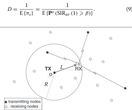
in [1,2]. In this paper, considering one-hop transmission in a multi-hopad hocnetworks, we choose the farthest receiving node strategy for balancing the hop numbers which is important for multi-hop performance. That is to say, a transmitting node will send packets to the farthest receiving node in its transmission radius. A realization of secondary network in one slot is shown in Figure 1; RX is the receiving node which is the farthest from the transmit-ting node TX within the transmission radiusR. And then all signal power received from other transmitting nodes are assumed to be the interference.
Since all receiving nodes follow a PPP with densityλSq, the probability distribution function of link distanceLis:
P(Lx)=PBo(x,R)∩rS= ∅|Bo(0,R)∩rS= ∅
=PBo(x,R)∩rS= ∅
PBo(0,x)∩rS= ∅
=e−λSqπ(R2−x2)1−e−λSqπx2 , 0<xR, (6)
and the probability density function ofLis
fL(x)=2λSqπxe−λSqπ(R
2−x2)
, 0<xR. (7)
The local delay
The local delayDofad hocnetwork is defined in [1] as the average number of time slots needed by a typical trans-mitting node u = o successfully sending packets to its receiving nodev=y, and:
D=E{inf{n1 :δ0(n)=1}}, (8)
whereδ0(n)indicates that (4) holds in time slotn. Letπc= Po(n), andπcis a variable which is irrelevant tonand equal to the probability of successful transmis-sion in the first time slot since the distribution of nodes is independent from time slot to time slot. And the local delay:
D= 1
E{πc} =
1 E{Po(SIR
uv(1)β)}
. (9)
TX L RX
transmitting nodes receiving nodes
R
Figure 1The selection strategy of receiving node.
The analysis of the local delay The local delay of CR network
Combining the definition of the local delay in (8) with the CR network model in this paper, the local delay of CR network is given in the following.
Let∂ndenote the event that the licensed channel is idle in time slotn, and a packet being successfully sent in time slotnis:
P1(n)=P(∂n=1)Po(n), (10)
wherePo(n)is given in (5). And then the number of trans-missionK needed for a packet sent from a transmitting node to the receiving node is valuable following a binomial distribution with parameterP1(n). DenoteD1as the local
delay of CR network which is the expectation ofK, and:
D1=E(K)= ∞
n=1
nE(P1(n)) n−1
l=1
(1−E(P1(l))).
(11)
Substituting (5) into (10), and based on (1), (11) can be rewritten as
D1= ∞
n=1
nP(S(nT)=0)p¯S n−1
l=1
(1−P(S(nT)=0)p¯S),
(12)
wherep¯S=E [Po(n)] is the expectation of probability for a successful transmission, which has nothing to do with time slotn. According to lemma 1 in [9], we have
¯ pS=E
EPotuhuvr−αβIuv
|L=r =Epe−λSpCαr2|L=r
. (13)
whereCα = α2πsin(2π/α)2β2/α . Putting (7) into (13), we have
¯ pS=E
pe−λSpCαr2
L=r
=
R 0
pe−λSpCαx2f L(x)dx
= pqπ
e−λSqπR2−e−λSpCαR2 (pCα−qπ) .
(14)
Comparing (11) with (9), the average probability of suc-cessful transmission E(P1(n))at time slotnis a function
related tonbecause of the existence of primary network (termP(∂n=1)).D1is derived by the law of total
prob-ability which is related to time slotn. Thus, we resort to the computer to show the relationship between D1 and
The local delay for two special cases
In some cases, the local delay can be approximated to be a value unrelated to the time slot. In the following, we will further analyze the local delay under two specifical cases of primary traffic.
The existence of the above expression is on the hypoth-esis of small amount of primary traffic, and time slotTis in units of microseconds, i.e.,(λ+μ)T <<1. In this case, the channel is almost regarded as idle state. The number of time slots needed by a successful transmission for a typ-ical node obeys the binomial distribution. The local delay of secondary network is a large amount of primary traffic. Since the packet arrival rate is always less than the departure rate which deduces to a stationary state of primary network at last. So, we have: delay is a geometric variable with parameter μp¯S
λ+μand
The optimization of CR local delay
According to the definition, the local delay is determined by both primary traffic and successful transmission prob-ability of the secondary network. In the following, we will give the optimization of the local delay about the three network parameters.
Theorem 1. The local delay D1 increases with increas-ing primary arrival rateλand decreasing departure rateμ when the other parameters are fixed.
Proof. The local delay is the expectation of a random variable with parameterP1(n). Observing (4), we find that
the term P(∂n=1)indicates the influence of the primary network. And:
P(∂n=1)=P(S(nT)=0)=P11(nT)
= λ+μμ +λ+λμe−(λ+μ)nT. (17)
Taking the derivative of (13) with respect toλandμ, we have:
It is obvious that P1(n) increases monotonously withλ
and decreases monotonously with μ. We complete the proof.
Theorem 2. When0<p< π+πCα, the necessary and suf-ficient condition for the local delay D1being concave with respect to the transmission probability of secondary nodes p is:
λS<
2p2Cα+q2π
pq(pCα−qπ) (π−Cα)R2. (18)
And we could get an optimal transmission probability in
0,π+πCα
to minimize the local delay by solving the equation in the following:
Proof. Since secondary nodes are overlaid with primary nodes, to prove the local delay is concave with respect to the transmission probability of secondary nodesp, all we have to do is to certify the second-order derivative of the average probability of successful transmissionp¯S in (13) which is less than zero, i.e.,d2p¯S
dp2<0. After calculat-ing and classifycalculat-ing, we getd2pS¯ dp2<0 whenλSmeets the requirements of (17) if 0 < p < π+πCα. Derivation is easy and omitted.
By solving the equationdpS¯ dp=0, we derive the opti-mal probability of successful transmission to minimize the local delay as shown in (18).
The proof is completed.
Note that the probability pis always less than 1, and thus, the optimization of local delay makes sense.
Theorem 3. When0 < p< π+πCα, the local delay D1is concave with respect to the density of secondary nodesλS. And the optimalλSis:
Numerical and simulation results
In this section, some numerical results are shown based on the theoretical analysis above. In order to verify the correctness of our analysis, we further give some sim-ulation results. Unless otherwise specified, the network parameters are set as shown in Table 1.
Simulation scenario settings
The primary network is modeled as the Markov pro-cess described in the ‘System model’ section. The arrival rateλand departure rateμare given in the figures. The original state of primary network is idle. The secondary nodes are uniformly distributed on a finite plane with area [0, 2, 000] m×[0, 2, 000] m. In each time slot, the num-ber of transmitting and receiving nodes follow a Poisson distribution with parameterλSpnodes/m2andλS(1−p) nodes/m2, respectively. Put a typical node on the center of the plane, the axis of which is [1, 000, 1, 000]. Consider the typical node begin to transmit packets with probabilityp once the channel state is detected to be idle in each slot. Regarding the number of time slots needed for a packet to be sent successfully as an example, the final simulation results are the mean value of 10,000 examples.
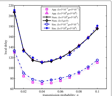
In Figure 2, we show the approximate (App.), numer-ical (Num.), and simulation (Sim.) results for the local delay with the transmission probability p varying from 0 to 0.1. We see that 1) the local delay is concave with respect to the transmission probabilitypwhenpandλS meet Theorem 2. In addition, an optimalpcan be found to minimize the local delay. Putting the parameters into (19), we solve the optimal transmission probability aspopt =
0.0405, which is the same as that in Figure 2. 2) The numerical result of the local delay withλ = 3,μ = 5) has a great difference between the approximate result of the local delay withλ = 0.003,μ = 0.005, while nearly equal to the approximate result of the local delay with
λ=3×10⁶,μ= 5×10⁶and very near the approximate solution of Equation 16. The local delay increases with the increasing primary traffic. But the increase of it slows down when the primary traffic reaches a certain value. 3) The simulation result is almost the same as the numerical result whenλ = 3×10⁶,μ = 5×10⁶. The simulation result is slight larger than the approximate result when the
Table 1 Parameter settings
Parameters Setting
Path loss factorα 4
Transmission radiusR 20 m
Time slotT 125μs
Decoding thresholdβ 10 dB
The density of secondary networkλS 0.005 nodes/m2
Transmission probabilityp 0.02
0.02 0.04 0.06 0.08 0.1
60 80 100 120 140 160 180 200 220
transmission probability: p
local delay
App. (λ=3*10−3,μ=5*10−3) App. (λ=3*106,μ=5*106)
Num. (λ=3*106,μ=5*106) Num. (λ=3,μ=5) Sim. (λ=3*10−3,μ=5*10−3) Sim. (λ=3*106,μ=5*106)
Figure 2The local delay versus transmission probabilityp.
primary traffic is zero. The simulation results prove the correctness of the theoretical analysis.
In Figure 3, we illustrate the approximate, numerical, and simulation results for the local delay with the den-sity of secondary nodesλSvarying from 0 to 0.01 whenp meets the requirement of Theorem 3. And we also could solve the optimalλSasλoptS = 0.0021 which agrees with the numerical results. Similar to Figure 2, the numerical result of the local delay withλ = 3,μ = 5 is almost the same as that withλ=3×10⁶,μ=5×10⁶and equal to
that in case 2 in the section ‘The local delay for two special cases’. This explains that the reciprocal of the local delay could be approximated to the product of the probability for idle channel state and success transmission probability for the secondary network without the primary network.
1 2 3 4 5 6 7 8 9 10
x 10−3
60 80 100 120 140 160 180 200 220 240 260
density of secondary nodes λS
local delay
App. (λ=3*10−3,μ=5*10−3)
App. (λ=3*106,μ=5*106) Num. (λ=3*106,μ=5*106) Num. (λ=3,μ=5) Sim. (λ=3*10−3,μ=5*10−3) Sim. (λ=3*106,μ=5*106)
1 2 3 4 5 6 7 8 9 10
x 10−3
100 120 140 160 180 200 220 240 260 280 300
density of secondary nodes λS
local delay
R=15 R=18 R=21
Figure 4The local delay versus density of secondary nodesλS
with varying transmission radiusR.
Similarly, the simulation result proves the correctness of the theoretical analysis.
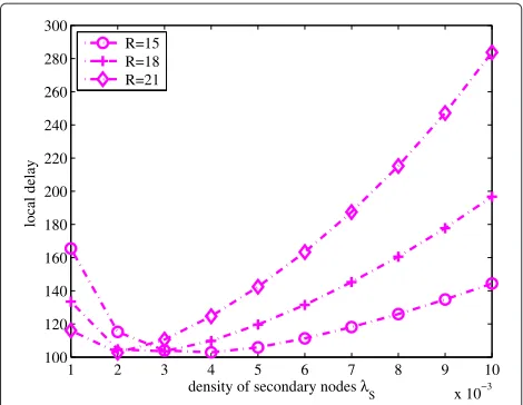
In Figure 4, we give the local delay versusλSwith three different transmission radii:R=15,R=18, andR=21. It is shown that the local delay increases with the increas-ingRwhenλSis small, while the opposite is the case when λS is larger. This is because when λS is small, whether a transmitting node could find a receiving node in its transmission radius affects the local delay greater than the interference coming from other transmitting nodes. Since the likelihood of existing receiving node is greater when Rgets larger and the probability of successful transmis-sion is larger, the local delay is smaller. The situation is on the contrary when the density of secondary nodes is larger and will not be covered here.
Conclusions
We conducted an analytical study of the local delay in cognitive radioad hoc networks. We modeled the occu-pancy of the licensed channel by the primary network as a Markov process, and the secondary nodes opportunisti-cally accessed the channel with the ALOHA protocol. The local delay is analyzed by employing the property of PPP in stochastic geometry.
We derived the analytical expression of the local delay and discussed the relationship between the local delay and some important network parameters which conclude the following: primary traffic (arrival and departure rates), transmission probability, and node density of the sec-ondary network. Both numerical and simulation results are obtained for different primary traffic. We drew a conclusion that the local delay in most cases could be approximated to that for significant primary traffic which is important for further research of end-to-end delay.
Competing interests
The authors declare that they have no competing interests.
Acknowledgements
This work was supported in part by the National Research Foundation for the Doctoral Program of Higher Education of China under Grant 20120005110007, the NSFC under Grant 61379159, and Beijing Natural Science Foundation under Grant 4122034.
Author details
1School of Electronics and Communication Engineering, Tianjin Normal
University, West Bin Shui Road, Xiqing District, 300387 Tianjin, China.2School of Information and Communication Engineering, Beijing University of Posts and Telecommunications, Xi Tu Cheng Road, Haidian District, 100876 Beijing, China.
Received: 22 October 2014 Accepted: 6 January 2015
References
1. F Baccelli, B Blaszczyszyn, inProceedings of IEEE INFOCOM. A new phase transition for local delays in MANETs (San Diego, Mar 2010), pp. 1–9 2. M Haenggi, inProceedings of IEEE ICC. Local delay in static and highly
mobile poisson networks with ALOHA (Cape Town, May 2010), pp. 1–5 3. M Haenggi, The local delay in Poisson networks. IEEE Trans. Inf. Theory.
59(3), 1788–1802 (2013)
4. F Baccelli, B Blaszczyszyn, P Muhlethaler, inProceedings of IEEE 6th International Symposium on Modeling and Optimization in Mobile, Ad Hoc, and Wireless Networks and Workshops (WiOPT). On the performance of time-space opportunistic routing in multihop mobile ad hoc networks (Berlin, Apr 2008), pp. 307–316
5. L Gao, R Zhang, C Yin, S Cui, Throughput and delay scaling in supportive two-tier networks. IEEE J. Sel. Areas Commun.30(2), 415–424 (2012) 6. J Lee, J Andrews, D Hong, Spectrum-sharing transmission capacity. IEEE
Trans. Wireless Commun.10(9), 3053–3063 (2011)
7. H Kim, KG Shin, Efficient discovery of spectrum opportunities with MAC-layer sensing in cognitive radio networks. IEEE Trans. Mobile Comput.7(5), 533–545 (2008)
8. WS D Stoyan, J Kendall,Mecke, Stochastic Geometry and Its Applications, 2nd ed. (John Wiley & Sons, Chichester, 1995)
9. F Baccelli, B Blaszczyszyn, P Muhlethaler, An Aloha protocol for multi-hop mobile wireless networks. IEEE Trans. Inf. Theory.52(2), 421–436 (2006)
Submit your manuscript to a
journal and benefi t from:
7Convenient online submission 7 Rigorous peer review
7Immediate publication on acceptance 7 Open access: articles freely available online 7High visibility within the fi eld
7 Retaining the copyright to your article