Optimal error estimate of the Legendre spectral approximation for space fractional reaction–advection–diffusion equation

R E S E A R C H

Open Access

Optimal error estimate of the Legendre

spectral approximation for space-fractional

reaction–advection–diffusion equation

Wenping Chen

1*

_{, Shujuan Lü}

1

_{, Hu Chen}

2

_{and Haiyu Liu}

1

*_{Correspondence:}

[email protected]

1_{School of Mathematics and}

Systems Science & LMIB, Beihang University, Beijing, China Full list of author information is available at the end of the article

Abstract

In this paper, we consider the space-fractional reaction–advection–diffusion equation with fractional diffusion and integer advection terms. By treating the first-order integer derivative as the composition of two Riemann–Liouville fractional derivative operators, we construct a fully discrete scheme by Legendre spectral method in a spatial and Crank–Nicolson scheme in temporal discretizations. Using thee right Riemann–Liouville fractional derivative, a novel duality argument is established, the optimal error estimate is proved to beO(

τ

2_+N–m_{) inL}2_{-norm. Numerical tests are} carried out to support the theoretical results, and the coefficient matrix with respect to first-order derivative obtained here is compared with that of traditional Legendre spectral method.

MSC: 65M12; 65M06; 65M70; 35R11

Keywords: Space-fractional reaction–advection–diffusion equation; Legendre spectral method; Crank-Nicolson scheme; Stability; Optimal error estimate

1 Introduction

Fractional differential equations (FDEs), in which standard temporal and/or spatial deriva-tive are replaced by fractional derivaderiva-tive operators, are widely used as a modeling tool and have a long history in many scientific and engineering fields, such as physics [1–3], finance [4–7], bioengineering [8–10], hydrology [11–14], and so on, for their cumulative memory effect.

There are several analytical methods to solve the FDEs, such as homotopy analysis method [15]. But in most cases, analytical methods do not work well on most of FDEs, so it is natural to resort to numerical methods. Up to now, there have been several numerical techniques to solve FDEs, such as finite difference method (FDM) [16–21], finite element method (FEM) [22–25], boundary elements method [26], spectral methods (SM) [27–36], etc. As far as we know, Lubich [20, 21] first introduced the idea of FDM to discretized fractional calculus. In [24], Roop introduced several equivalent fractional Sobolev spaces, and developed a theoretical framework for the Galerkin finite element approximation to steady-state and time-dependent fractional advection dispersion equations with Dirichlet boundary conditions.

The fractional derivative is essentially a global differential operator, whereas FDM and FEM are inherently local methods that lack the capability to deal with the fractional deriva-tive effecderiva-tively. Therefore, it is natural to consider a global method. Spectral method is well known for its global feature and high order accuracy. To compute the fractional dif-ferential equation accurately, spectral method is a suitable choice for its nature. Lin and Xu [35] proposed a finite difference scheme in time and Legendre collocation spectral method in space for the time-fractional diffusion equation in Caputo sense. In [33, 34], Li and Xu developed a time-space spectral method for the time-fractional diffusion equa-tion, and spectral accuracy was received both in time and space. Li et al. [32] proposed the spectral collocation method to solve the fractional initial value problems and bound-ary value problems. Bueno-Orovio et al. [27] introduced Fourier spectral methods for the space fractional reaction-diffusion equations described by the fractional Laplacian in bounded domain. In [36], Nie et al. considered the backward Euler scheme in time and Galerkin-Legendre spectral method in space for spatial-fractional diffusion equations on a bounded interval, the convergence order wasO(τ+Nα–m_{) inL}2_{-norm. Huang et al. [31]}

combined the second order finite difference method in time and the spectral Galerkin method in space for space-fractional diffusion equations, the convergence order of the proposed method was proved to beO(τ2+Nα–m_{) inL}2_-norm.

The model problem considered in this paper is the space-fractional reaction–advection– diffusion equation (SFRADE):

ut–K1–1D2xαu+K2ux+K3u=f(x,t), (x,t)∈D=Ω×I, (1)

subject to the following initial and boundary conditions:

u(x, 0) =u0(x), x∈Ω, (2)

u(±1,t) = 0, t∈I, (3)

where Ω= (–1, 1), I= (0,T],α∈(1/2, 1].K1> 0,Ki≥0 (i= 2, 3) are diffusion, advec-tion, and reaction coefficients, respectively.K1–Cp(K2+K3) > 0,Cpis a positive constant (see below). The fractional order operator–1D2xαis the left Riemann–Liouville fractional derivative of order 2α with respect tox, commonly referred to as an anomalous diffu-sion operator. If we takeα= 1 in (1), it is the integer diffusion operator, and the classical reaction–advection–diffusion equation is obtained. The key difference between the frac-tional operator and the usual one is that the former is nonlocal.

Definition 1(Riemann–Liouville (R–L) fractional integral [37, 38]) Letvbe a function defined on (a,b), andσ> 0.

Then the left Riemann–Liouville fractional integral of orderσis defined to be

aD–xσv(x) = 1

Γ(σ) x

a

(x–ξ)σ–1v(ξ) dξ, x>a.

The right Riemann–Liouville fractional integral of orderσ is defined to be

xD–bσv(x) = 1

Γ(σ) b

x

Definition 2(Riemann–Liouville (R–L) fractional derivative [37, 38]) Letvbe a function

defined on (a,b),β> 0,nbe the smallest integer greater thanβ(n– 1≤β<n), andσ=

n–β.

Then the left fractional derivative of orderβis defined to be

aDβxv(x) =DnaD–xσv(x) = 1

Γ(σ) dn dxn

x

a

(x–ξ)σ–1v(ξ) dξ, x∈(a,b).

The right fractional derivative of orderβis defined to be

xDβbv(x) = (–D)nxD–bσv(x) = (–1)n

Γ(σ) dn dxn

b

x

(ξ–x)σ–1v(ξ) dξ, x∈(a,b).

In this paper, we consider the first order derivative as composition of two 1/2-order left R–L derivatives for the advection term of (1)–(3) according to the property of R–L frac-tional derivative as that in [39]. We also establish a duality argument by using the right R–L fractional derivative, the purpose is to construct an efficient approach by applying the Leg-endre spectral method in spatial and Crank–Nicolson scheme in temporal discretizations such that it can be implemented efficiently and has an optimal convergence rate.

The organization of the paper is as follows. We commence by reviewing some prelimi-naries of fractional order functional spaces endowed with inner products and norms, and the weak formulation for the space-fractional reaction–advection–diffusion equation is given in the next section. The fully discrete spectral scheme by applying Legendre spec-tral method to the spatial component and Crank–Nicolson difference scheme to time derivative is constructed, and the existence and uniqueness of the fully discrete scheme are proved by the Lax–Milgram theorem in Sect. 3. In Sect. 4, by constructing a fractional duality argument, we carry out the stability and optimal convergence analysis of the fully discrete scheme, respectively. In Sect. 5, we present some numerical experiments, which support the theoretical estimates. We conclude by summary and discussion of our method for fractional differential equation in the last section.

2 Preliminaries

In this section, we introduce some definitions and notations of fractional derivative spaces endowed with inner products and norms, then give some basic properties of fractional derivative, which will be used in the context.

The L2_{(Ω) inner product is denoted by (·,·) and theL}p_{(Ω) norm by ·}

Lp with the special case ofL2(Ω) andL∞(Ω) norms being written as · and · ∞, respectively. For

k∈N, we denote the semi-norm and the norm associated with the Sobolev spaceHk_(Ω) by| · |kand · k, respectively. For nonnegative real numberr∈R+\Z+, we useHr(Ω) to denote the fractional Sobolev spaces, the semi-norm| · |rand the norm · ras defined below.

Definition 3(see [24, 40]) Letr> 0. Define the semi-norm

|u|r=|ω|ruˆ_L2_(R)=

R|ω|

2r_|ˆu|2_dω

1 2

and the norm

ur=

u2+|u|2_r12_,

whereuˆ= _Ru(x)e–iωx_{dxdenotes the Fourier transform ofu, the transform variableωis} a real number. DefineHr

0(Ω) as the closure ofC∞0 (Ω) inHr(Ω) with respect to the norm

· r, and useH–r(Ω) to denote the dual space ofH0r(Ω), with the norm denoted by · –r.

Remark1 (see [24]) Letu˜be the expansion ofuby zero outside ofΩ, then|u|r=|˜u|Hr_(R). Throughout the paper, we useCto denote a generic nonnegative constant whose actual value may change from line to line.

Next, we introduce some useful fractional derivative spaces and related properties, which are used in the formulation of the numerical analysis, one can refer to [24, 40] for more details.

Definition 4(see [24, 40]) Letμ> 0. Define the semi-norm

|u|J_Lμ(Ω)=–1Dμxu,

and the norm

uJ_Lμ(Ω)=

u2_+|u|2

J_Lμ(Ω)

1 2_.

DenoteJ_Lμ_,0(Ω) as the closure ofC₀∞(Ω) with respect to the norm · _Jμ L(Ω).

Definition 5(see [24, 40]) Letμ> 0. Define the semi-norm

|u|J_Rμ(Ω)=xDμ1u,

and the norm

uJ_Rμ(Ω)=

u2_+|u|2

J_Rμ(Ω)

1 2_.

DenoteJ_Rμ_,0(Ω) as the closure ofC₀∞(Ω) with respect to the norm · _Jμ R(Ω).

Definition 6(see [24, 40]) Letμ> 0,μ=n–1

2,n∈N. Define the semi-norm

|u|JSμ(Ω)=–1D

μ

xu,xDμ1u

1 2_,

and the norm

u_Jμ S(Ω)=

u2+|u|2_Jμ S(Ω)

1 2_.

Lemma 1(see [24, 40]) Letμ> 0,μ=n– 1/2,n∈N.Then spaces J_Lμ_,0(Ω),J_Rμ_,0(Ω),J_Sμ_,0(Ω),

and H₀μ(Ω)are equal,with equivalent semi-norms and norms.

Remark2 If the domainΩin Definitions 4–6 is replaced by the entire lineR, the corre-sponding semi-norms should be denoted, respectively, by

⎧ ⎪ ⎪ ⎨ ⎪ ⎪ ⎩

|u|Jμ_L(R)=–∞DμxuL2_(R),

|u|Jμ_R(R)=xDμ∞uL2_(R),

|u|Jμ_S(R)= (|(–∞Dμxu,xDμ∞u)|)

1 2_.

LetJ_Lμ(R),J_Rμ(R),J_Sμ(R), andHμ_{(R) denote the closure ofC}∞

0 (R) with respect touJ_Lμ(R),

uJRμ(R),uJ μ

S(R), anduHμ(R), respectively.

Lemma 2(see [24, 40]) Letμ> 0,μ=n– 1/2,n∈N.Then spaces J_Lμ(R),J_Rμ(R),J_Sμ(R),and Hμ_{(R)are equal,with equivalent semi-norms and norms.}

Lemma 3(see [24, 40]) Letμ> 0.A function u∈L2(R)belongs to J_Lμ(R)if and only if |ω|μ_uˆ∈L2_{(R),specifically|u|}

J_Lμ(R)=|ω|μuˆ L2_(R)=|u|_Hμ_(R).Similarly,|u|

J_Rμ(R)=|u|Hμ_(R).

Lemma 4(see [24, 40]) Letμ> 0be given.Then

–1Dμxu,xDμ1u

=–∞Dμxu˜,xDμ∞u˜=cos(π μ)–∞Dμxu˜

2

L2_(R)=cos(π μ)xDμ∞u˜2L2_(R).

Hence we have the following relations.

Lemma 5(see [24, 40]) Letμ> 0,Ω= (–1, 1),u∈J_Lμ_,0(Ω)∩J_Rμ_,0(Ω).Then

–1Dμxu,xDμ1u

=cos(π μ)|u|μ.

Proof We can get the result by Remark 1 and Lemmas 3, 4, immediately.

Lemma 6(Fractional Poincaré–Friedrichs inequality [40]) For u∈J_Lμ_,0(Ω),

u ≤C|u|_Jμ L(Ω),

and for0 <s<μ,

|u|Js

L(Ω)≤C|u|JLμ(Ω).

The results for J_Rμ_,0(Ω)follow analogously.For u∈H₀μ(Ω),

u ≤Cp|u|μ,

and for0 <s<μ,s=n– 1/2,n∈N,

Via integration by parts, one can verify the following readily.

Now, we introduce some space-time functional spaces. LetE be a Hilbert space, we define the spaceL2_{(0,T;E) as}

and similarly we can define some other spaces for space-time functions.

We definea(u,v) = –K1(–1Dxαu,xDα1v) +K2(–1D

the linearity of the left and right R–L derivatives, we can verify readily thata(·,·) is a bi-linear form. The variational formulation of equation (1) with the homogeneous bound-ary condition is as follows: Let f ∈L2_{(D) and u}

Proof Hölder’s inequality, Lemmas 1 and 6 yield

a(u,v)≤K1–1DxαuxDα1v+K2–1D

On the other hand, by Remark 3, Lemmas 1-2, 5-6, we have

≥CminK1|cosπ α|,K3

u2

α

C2u2α, ∀u∈H α 0(Ω),

viz.,a(·,·) is coercive onHα 0(Ω).

The proof of the lemma is completed.

According to the above lemma on the continuity and coercivity of the bilinear form

a(·,·), the existence and uniqueness of solution for the weak form above (4)–(5) could be proved.

Theorem 1 Let u0∈L2(Ω), f ∈L2(D).Then(4)–(5)has a unique solution u∈L2(0,T;

Hα

0(Ω))∩C0([0,T];L2(Ω)).Furthermore, ∂∂ut ∈L

2_(0,T;H–α_(Ω))and

u2+C

t

0

u2_αds≤ u02+C

t

0

f2ds, ∀t∈[0,T]. (6)

Proof Assume that{φk(x),k= 0, 1, . . . ,N}is the complete orthogonal basis ofV=H0α(Ω).

DefineVN=span{φ0, . . . ,φN}, then we get the approximation problem: for eacht∈[0,T], findUN(x,t)∈VNsuch that

_d

dt(UN(t),v) +a(UN(t),v) = (f,v), ∀v∈V, (7)

UN(0) =u0,N= N

j=0ρjφj. (8)

Letv=φj,UN=Nk=0ck(t)φk, we have the following linear ordinary differential equation:

d

dtcj(t)(φj,φj) +

N

k=0

a(φk,φj)ck(t) = (f,φj), j= 0, 1, . . . ,N. (9)

Since (φj,φj) > 0,∀j= 0, 1, . . . ,N, there exists a unique solutioncN= (cN0,cN1, . . . ,cNN)Tto (9) andUN∈H1(0,T;V).

ChoosingUN(t) as a test function, we get

d

dtUN(t),UN(t)

+aUN(t),UN(t)

=f(t),UN(t)

.

Then, by the coercivity ofa(·,·), we obtain

1 2

d

dtUN(t)

2

+C2UN(t)

2

α≤ fUN(t)≤

1 2C2f

2₊C2

2 UN(t)

2 α.

Integrating the inequality over (0,t),t∈(0,T], we have

_UN(t)2+C2

t

0

_UN(t)_α2ds≤ u02+C

t

0

f2_{ds. (10)}

ThusUN(x,t)∈L∞(0,T;L2(Ω))∩L2(0,T;V). There exists a subsequence (still denoted by

i.e., there existsu˜∈L∞(0,T;L2_(Ω))∩L2_{(0,T;V) such that}

whereDα_andD1_{2 are left/right Riemann–Liouville fractional derivatives, respectively. Let}

φ(t)∈C1[0,T] withφ(T) = 0, multiplying (7) byφ(t), integrating with respect tot, and using integration by parts, we get

–

integration by parts, we obtain

–

Comparing (11) with (13), we get

˜

u(0),v= (u0,v), ∀v∈V.

Thusu˜(0) =u0, the existence of the solution of (4)–(5) is established. LetN→ ∞in (10),

we obtain estimate (6).

u∈L2_{(0,T;V) leads to –K}

1–1D2xαu+K2ux+K3u∈L2(0,T;V), whereV is the dual

space ofV. Byf∈L2(D)⊂L2(0,T;V), we getd_du_t ∈L2(0,T;V) andu∈H1(0,T;V), which means thatu∈C0([0,T];L2(Ω)).

From (6) we have

w2_+C

2

t

0

w2

αdt≤0,

which impliesw= 0, i.e.,u1=u. The proof of the theorem is completed.

3 Existence and uniqueness of the fully discrete scheme

In this section, we study the existence and uniqueness of the fully spectral discrete scheme of (1)–(3). By introducing some lemmas and tools, we prove that the fully discrete scheme has a unique solution.

LetPN(Ω) be the set of all algebraic polynomials defined on domainΩwith the degree less than or equal toN∈Z+.V_N0 =PN(Ω)∩H01(Ω). Letτ be the step size for timet,tk=

kτ,k= 0, 1, . . . ,nT, andT=nTτ,tk–1₂ = (tk+tk–1)/2. For convenience, we introduce the

following notations for the functionu(x,t):

uk=uk(·) =u(·,tk), uk–

1 2 _=u(t

k–1₂),

¯

∂tuk=

uk–uk–1

τ , u

ˆ

k₌uk+uk–1

2 .

Due to homogeneous boundary conditions, we adopt Legendre–Gauss–Lobatto (LGL) points here. LetIN:C(Ω¯)→PNbe the interpolating operator associated with LGL points.

INu(xi) =u(xi), i= 0, 1, . . . ,N,

wherexi∈ ¯Ωare LGL points.

For the time advance, the Crank–Nicolson scheme will be used to discrete the tempo-ral derivative of (1). We can obtain the fully discrete Crank–Nicolson–Legendre specttempo-ral method for (1)–(3): finduk

N∈VN0, 1≤k≤nT, such that ⎧

⎨ ⎩

(∂¯tukN,v) +a(u ˆ k

N,v) = (fk–

1

2_,v), ∀v∈_V0

N,

u0

N=u0N,

(14)

whereu0N∈VN0 is an approximation ofu0in the spaceVN0.

Now, we consider the existence and uniqueness of the Crank–Nicolson fully discrete scheme (14), we have the following theorem.

Theorem 2 Let u0∈L2(Ω),f ∈L2(D).The Crank–Nicolson fully discrete scheme(14)has

a unique solution uk_N ∈V_N0.

Proof Rewrite scheme (14) as the following equivalent form:

uk_N,v+τ 2a

uk_N,v=uk_N–1,v–τ 2a

uk_N–1,v+τfk–12_,v.

For simplicity, we denoteA(u,v) = (u,v) +τ₂a(u,v),F(v) = (u_Nk–1,v) –τ₂a(uk_N–1,v) +τ(fk–12_,v).

On the one hand, via Lemma 8, we have

and On the other hand, by virtue of Hölder’s inequality, we deduce that

F(v)=uk_N–1,v–τ

Thus the existence and uniqueness of (14) are ensured by the Lax–Milgram theorem.

The proof is completed.

4 Stability and convergence of the fully discrete scheme

In this section, we consider the stability and convergence analysis for the fully discrete scheme (14). Let us first consider the stability of scheme (14), we have the following result.

Theorem 3 The fully discrete scheme(14)is unconditionally stable.

Proof Takingv=uk_Nˆ in (14), we obtain

For the left-hand side of (15), we infer that

_¯

On the other hand, for the right-hand side of (15), we have

Bringing the above two inequalities into (15), and summing forkfrom 1 ton, we deduce that

The theorem is proved.

For the following projectorΠ_N1,0, one can be referred to [41] for more details. LetΠ_N1,0:H₀1(Ω) →V_N0 be the orthogonal projection operator such that

∂x

u–Π_N1,0u,∂xϕN

= 0, ∀ϕN∈VN0.

For the operatorΠ_N1,0, we have the following estimate.

Lemma 9(see [41]) Let s be a real number.For any nonnegative real number r, 0≤s≤ r,there exists a positive constant C depending only on r such that,for any function u in Hs

0(Ω)∩Hr(Ω),the following estimate holds:

u–Π_N1,0u_s≤CNs–rur.

Define the projectorΠ_Nα,0:Hα

0(Ω) →VN0 such that

au–Π_Nα,0u,v= 0, ∀v∈V_N0. (16)

By virtue of (16) and the continuity and coercivity of the bilinear forma(·,·), we have

Cu–Π_Nα,0u2_α≤au–Π_Nα,0u,u–Π_Nα,0u

=au–Π_Nα,0u,u–Π_N1,0u

≤Cu–Π_Nα,0u_αu–Π_N1,0u_α, ∀u∈V_N0.

Therefore, by Lemma 9, we get

u–Π_Nα,0u_α≤Cu–Π_N1,0u_α≤CNα–r_u

r, α≤r.

We next estimate the erroru–Π_Nα,0uusing a duality argument. For anyg∈L2_{(Ω), we}

consider the auxiliary problem ⎧

⎨ ⎩

–K1xD21αw–K2wx+K3w=g, inΩ,

w= 0, on∂Ω. (17)

We can get that

w2α≤Cg. (18)

The weak form of (17) is as follows:

a(ϕ,w) = (g,ϕ), ∀ϕ∈H₀α(Ω). Takingϕ=u–Π_Nα,0u, we obtain

g,u–Π_Nα,0u=au–Π_Nα,0u,w

≤u–Π_Nα,0u_αw–Π_N1,0w_α

Using (18) and (19), we have

u–Π_Nα,0u= sup

g∈L2_(Ω),g=0

|(g,u–Π_Nα,0u)|

g ≤CN–rur. (20)

Discrete Gronwall’s inequality is a useful tool in the convergence analysis.

Lemma 10(Discrete Gronwall’s inequality[42]) Letτ,B,ai,bi, ci,γi(integers i≥0)be

nonnegative numbers such that

an+τ

Now, we consider the convergence of the fully discrete scheme.

Theorem 4 Let1/2 <α< 1,u and uk

N be the solutions of(1)–(3)and(14),respectively.

Assume that ut∈L2(0,T;Hm(Ω)),utt∈L2(0,T;Hα(Ω)),uttt∈L2(0,T;L2(Ω)),and u0∈

Hm_{(Ω),m>α.Then there exists a positive constant C independent of k,τ,and N such that} uk–uk_N≤Cτ2+N–m, 0≤k≤nT.

Proof Settinge=u–Π_Nα,0uandη=Π_Nα,0u–uN, by (1)–(3), (14) and the definition of projectorΠ_Nα,0, we get the error equation below: for all

⎧

For the left-hand side of (23), we note that

Thus for the left-hand side of (23), we obtain

Next we estimate terms on the right-hand side of (23). By Hölder’s inequality and Young’s inequality, we have

According to Hölder’s inequality, we deduce that

∂¯tek

Substituting (26) into (25), we get

∂¯tek,ηkˆ≤

Via Taylor’s theorem with integral remainder and Young’s inequality, we infer that

∂¯tuk–u

By virtue of Hölder’s inequality, we obtain

Substituting (29)–(30) into (28), we get

For the last term on the right-hand side of (23), we have

Via Taylor’s formula and Hölder’s inequality, we deduce that

ukˆ–uk–122

Inserting (33) into (32), we obtain

aukˆ_–uk–12_,ηkˆ≤C2

Moreover, by virtue of (20), we obtain

en2=UN–ΠNα,0UN2≤CN–2mUN2m=CN–2m

Finally, combining the formulae (36) and (37), we get the error estimate.

5 Numerical experiments

In this section, we present numerical results obtained by the proposed method.

5.1 Implementation

Now, we give the implementation of the fully discrete system (14).

LetLk(x) be the Legendre polynomial of degreekwith the following recursive relations (see [43]):

L0(x) = 1, L1(x) =x, (k+ 1)Lk+1(x) = (2k+ 1)xLk(x) +kLk–1(x), (38)

L_k+1(x) –L_k–1(x) = (2k+ 1)Lk(x), k≥1. (39)

A detailed discussion of the properties of Legendre polynomials is furnished in [44].

Lemma 11([31]) If0 <μ< 1,we have

The function spaceV0

Ncan be expressed asVN0=span{φi(x) :i= 1, 2, . . . ,N– 1}, in which

and

Substituting (42), (43) into (41) and lettingv=φj, we obtain the matrix form of the discrete scheme as follows:

In the numerical experiments, we use Jacobi–Gauss–Lobatto quadrature to calculate the elementSα

By virtue of Lemma 11, we obtain

Table 1 max|a 1 2

ij|andL1,L2,L∞norms ofA 1

2_=S12_{–Sfor differentN}

N max|a

1 2

ij| L1norm L2norm L∞norm

10 8.8818e–15 2.9421e–14 1.8203e–14 2.6201e–14 50 9.1038e–14 4.1622e–13 1.5942e–13 4.0790e–13 90 5.9908e–13 1.7258e–12 9.2418e–13 1.8320e–12

Table 2 max|a0_ij|andL1,L2,L∞norms ofA0=S0–Mfor differentN

N max_|a0ij| L1norm L2norm L∞norm

10 7.5495e–15 1.1657e–14 8.1202e–15 1.1657e–14 50 7.9936e–15 2.5934e–14 9.6391e–15 2.5879e–14 90 1.7186e–13 2.3348e–13 1.7794e–13 2.3354e–13

where{xk},k= 0, 1, . . . ,M, are the Jacobi–Gauss–Lobatto points with respect to the weight functionω–α,–α_{(x) = (1 +x)}–α_{(1 –x)}–α_{. IfM≥N+ 1, the numerical integration (45) is exact}

for all 0≤i,j≤N. We can also use Jacobi–Gauss or Jacobi–Guass–Radau quadrature to calculateSα

ij[45].

Remark4 The element of coefficient matrixS∈R(N–1)×(N–1)_{, corresponding to the}

advec-tion termux, is calculated bySij= (∂xφj,φi) (1≤i,j≤N– 1) in the traditional fully discrete Legendre spectral scheme case. In our numerical scheme, we calculate it in the same way as that of fractional diffusion term withα=1₂. LetA12 _{= (a}

1 2

ij) =S

1

2 _{–S, Table 1 lists the}

maximum absolute value|a

1 2

ij|as well asL1,L2, andL∞norms of the matrixA

1

2 _for

differ-entN, respectively. It indicates that matrixS12 obtained by our scheme and matrixSare

considerably similar, so the approach we adopt here is suitable.

Remark5 In fact, our numerical scheme is also right to calculate the coefficient matrix

Mcorresponding to the reaction termuwithα= 0. LetA0_{= (a}0

ij) =S0–M. Table 2 lists the maximum absolute value|a0

ij|andL1,L2, andL∞norms of the matrixA0for different values ofN.

5.2 Numerical example

Example1 Consider the following SFRADE:

⎧ ⎪ ⎪ ⎨ ⎪ ⎪ ⎩

ut––1D2xαu+ux+u=f(x,t), (x,t)∈D=Ω×I,

u(x, 0) =eβ_(x2_{– 1)}2_{, x∈Ω,}

u(±1,t) = 0, t∈I,

(46)

whereΩ= (–1, 1),I= (0, 1], and

f(x,t)

= (α+ 1)eαt+β_x2_{– 1}2

+ 4eαt+β_xx2_{– 1}

– 8e

αt+β

Γ(5 – 2α)(x+ 1)

2–2α_{3(x+ 1)}2_{– 3(4 – 2α)(x+ 1) + (4 – 2α)(3 – 2α).}

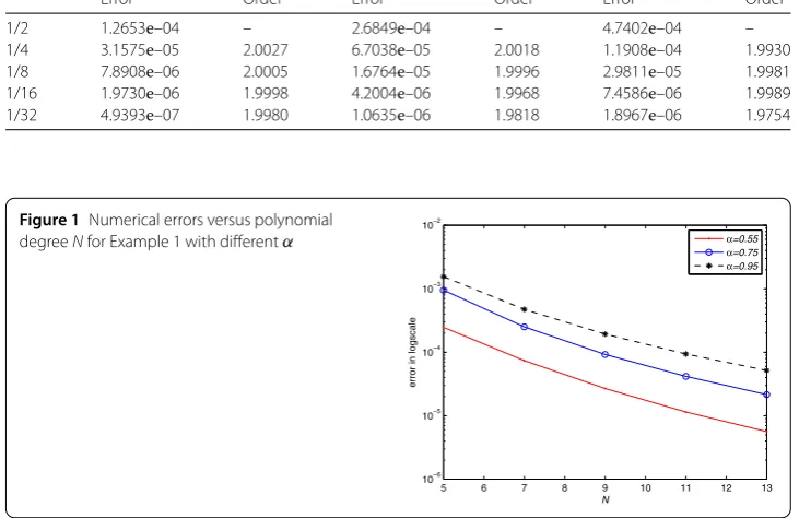
Table 3 TheL2_{errors and temporal convergence order with differentαandτfor Example 1,N= 50}

τ α= 0.55 α= 0.75 α= 0.95

Error Order Error Order Error Order

1/2 1.2653e–04 – 2.6849e–04 – 4.7402e–04 –

1/4 3.1575e–05 2.0027 6.7038e–05 2.0018 1.1908e–04 1.9930

1/8 7.8908e–06 2.0005 1.6764e–05 1.9996 2.9811e–05 1.9981

1/16 1.9730e–06 1.9998 4.2004e–06 1.9968 7.4586e–06 1.9989

1/32 4.9393e–07 1.9980 1.0635e–06 1.9818 1.8967e–06 1.9754

Figure 1Numerical errors versus polynomial degreeNfor Example 1 with differentα

To confirm the temporal accuracy, we chooseN= 50, which is large enough such that the spatial error is negligible compared with the temporal error. Table 3 lists the errors

u–uNand temporal convergence rates. From the table, we can check that temporal convergence order, almost second-order, is in accordance with the theoretical result in Theorem 4.

Next, we investigate the spatial discretization error. We takeτ= 0.001 so that the tem-poral discretization error is negligible compared with the spatial discretization error. As shown in Fig. 1, theL2_{errors of the numerical solution with different values ofαdecay}

exponentially in an approximate line as the polynomial degreeNincreases. Solutionuis sufficiently smooth with respect to spatial variablex, thus the numerical result coincides with Theorem 4.

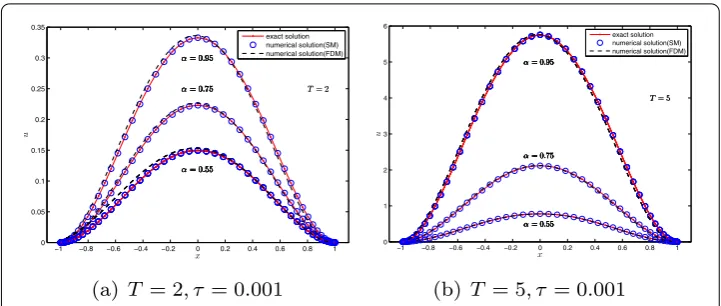
In Fig. 2, comparisons between the exact solution and the numerical solutions of the present method and the finite difference method are presented at various values of the final time T andα, respectively, where N= 50. It can be seen that numerical results of the spectral method much better coincide with the exact solution than those of the finite difference method. This illustrates that the spectral method is a high accuracy method.

Example2 Consider the following SFRADE:

⎧ ⎪ ⎪ ⎪ ⎨ ⎪ ⎪ ⎪ ⎩

ut– 3–1D2xαu+ 2ux=f(x,t), (x,t)∈D=Ω×I,

u(x, 0) = (1 –x)(x+ 1)4_{, x∈Ω,}

u(±1,t) = 0, t∈I,

Figure 2Comparisons of the exact solution with the numerical solutions of spectral method and finite difference method for Example 1 with differentαandT, whereN= 50

Figure 3The numerical and the exact solution at

T= 1 for Example 2, takingN= 50

whereΩ= (–1, 1),I= (0, 1], and

f(x,t) =

π

4 cos

πt

4 +K3sin

πt

4

(1 –x)(x+ 1)4+K2sin

πt

4 (x+ 1)

3_{(3 – 5x)}

– 4!K1

Γ(6 – 2α)sin

πt

4 (x+ 1)

4–2α_{(5 – 5x– 4α).}

It is easy to verify that the exact solution of (47) isu(x,t) =sinπ₄t(1 –x)(x+ 1)4. The comparisons of the numerical and the exact solution of problem (47) att= 1 are shown in Fig. 3. In this case, we take the time step sizeτ= 0.0001 and the degree of interpolation polynomial in spatial directionN= 50. It can be seen that our numerical results are in excellent agreement with the exact solution.

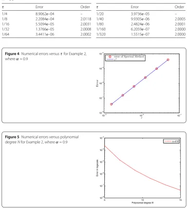
We takeN= 50, a value large enough such that the spatial discretization errors are neg-ligible compared with the temporal errors, we choose different time step sizeτ to obtain the numerical convergence order in time list in Table 4. We consider the errors as a func-tion ofτ, and plot the log-log graph withT= 1 andα= 0.9 in Fig. 4, it coincides withτ2_.

Table 4 TheL2_{errors and temporal convergence order with differentτ for Example 2,α= 0.9,}

N= 50

τ Error Order

1/4 8.9062e–04 –

1/8 2.2084e–04 2.0118

1/16 5.5094e–05 2.0031

1/32 1.3766e–05 2.0008

1/64 3.4411e–06 2.0002

τ Error Order

1/20 3.9736e–05 –

1/40 9.9305e–06 2.0005

1/80 2.4824e–06 2.0001

1/160 6.2059e–07 2.0000

1/320 1.5515e–07 2.0000

Figure 4Numerical errors versusτfor Example 2, whereα= 0.9

Figure 5Numerical errors versus polynomial degreeNfor Example 2, whereα= 0.9

In Fig. 5, we plot the logarithm of errorsu–uNas a function of the polynomial de-greeNatT= 1 withα= 0.9. Figure 5 demonstrates that our method has spectral accuracy in space for this problem. Obviously, the exponential convergence in spatial discretization can be seen from the figure which shows almost linear curves. The above numerical exper-iments state that it is effective and feasible to use spectral method to solve space-fractional reaction–advection–diffusion equations.

6 Conclusions

deriva-tive case as well as the Riesz fractional derivaderiva-tive. The methodology we present here can also be suitable for problems in the 2-D and 3-D cases, and a discrete scheme with various spectral methods and different temporal discretizations will be considered in our future work.

Acknowledgements

The research is supported by the National Natural Science Foundation of China (Grant Nos. 11672011, 11272024).

Competing interests

The authors declare that they have no competing interests.

Authors’ contributions

WC and SL contributed equally to this work. All authors read and approved the final manuscript.

Author details

1_{School of Mathematics and Systems Science & LMIB, Beihang University, Beijing, China.}2_{Beijing Computational Science}

Research Center, Beijing, China.

Publisher’s Note

Springer Nature remains neutral with regard to jurisdictional claims in published maps and institutional affiliations.

Received: 22 November 2017 Accepted: 20 March 2018 References

1. Hilfer, R.: Application of Fractional Calculus in Physics. World Scientific, Singapore (2000)

2. Uchaikin, V.V.: Fractional Derivatives for Physicists and Engineers, Vol. I: Background and Theory. Higher Education Press, Beijing; Springer, Berlin (2013)

3. Uchaikin, V.V.: Fractional Derivatives for Physicists and Engineers, Vol. II: Applications. Higher Education Press, Beijing; Springer, Berlin (2013)

4. Gorenflo, R., Mainardi, F., Scalas, E., Raberdo, M.: Fractional calculus and continuous-time finance, III: the diffusion limit. In: Mathematical Finance. Trends in Math., pp. 171–180. Birkhäuser, Basel (2001)

5. Meerschaert, M.M., Scalas, E.: Coupled continuous time random walks in finance. Physica A370, 114–118 (2006) 6. Picozzi, S., West, B.: Fractional Langevin model of memory in financial markets. Phys. Rev. E66, 046118 (2002) 7. Raberto, M., Scalas, E., Mainardi, F.: Waiting-times and returns in high-frequency financial data: an empirical study.

Physica A314, 749–755 (2002)

8. Magin, R.L.: Fractional calculus in bioengineering. Crit. Rev. Biomed. Eng.32, 1–104 (2004) 9. Magin, R.L.: Fractional calculus in bioengineering, part 2. Crit. Rev. Biomed. Eng.32, 105–193 (2004) 10. Magin, R.L.: Fractional calculus in bioengineering, part 3. Crit. Rev. Biomed. Eng.32, 195–378 (2004)

11. Adams, E.E., Gelhar, L.W.: Field study of dispersion in a heterogeneous aquifer: 2. Spatial moment analysis. Water Resour. Res.28, 3293–3307 (1992)

12. Benson, D.A., Wheatcraft, S.W., Meerschaert, M.M.: Application of a fractional advection–dispersion equation. Water Resour. Res.36, 1403–1412 (2000)

13. Benson, D.A., Wheatcraft, S.W., Meerschaert, M.M.: The fractional-order governing equation of Lévy motion. Water Resour. Res.36, 1413–1423 (2000)

14. Liu, F., Anh, V., Turner, I.: Numerical solution of space fractional Fokker–Planck equation. J. Comput. Appl. Math.166, 209–219 (2004)

15. Dehghan, M., Manafian, J., Saadatmandi, A.: The solution of the linear fractional partial differential equations using the homotopy analysis method. Z. Naturforsch. A65a, 935–949 (2010)

16. Alikhanov, A.A.: A new difference scheme for the time fractional diffusion equation. J. Comput. Phys.280, 424–438 (2015)

17. Alikhanov, A.A.: Stability and convergence of difference schemes approximating a two-parameter nonlocal boundary value problem for time-fractional diffusion equation. Comput. Math. Model.26, 252–272 (2015)

18. Chen, S., Liu, F., Zhuang, P., Anh, V.: Finite difference approximations for the fractional Fokker–Planck equation. Appl. Math. Model.33, 256–273 (2009)

19. Liu, F., Zhuang, P., Anh, V., Turner, I., Burrage, K.: Stability and convergence of the difference methods for the space-time fractional advection–diffusion equation. Appl. Math. Comput.191, 12–20 (2007)

20. Lubich, C.: On the stability of linear multistep methods for Volterra convolution equations. IMA J. Numer. Anal.3, 439–465 (1983)

21. Lubich, C.: Discretized fractional calculus. SIAM J. Math. Anal.17, 704–719 (1986)

22. Ervin, V.J., Heuer, N., Roop, J.P.: Numerical approximation of a time dependent, nonlinear, space-fractional diffusion equation. SIAM J. Numer. Anal.45, 572–591 (2007)

23. Jin, B., Lazarov, R., Pasciak, J., Zhou, Z.: Error analysis of a finite element method for the space-fractional parabolic equation. SIAM J. Numer. Anal.52, 2272–2294 (2015)

24. Roop, J.P.: Variational Solution of the Fractional Advection Dispersion Equation. PhD thesis, Clemson University, Clemson, SC (2004)

26. Dehghan, M., Safarpoor, M.: The dual reciprocity boundary integral equation technique to solve a class of the linear and nonlinear fractional partial differential equations. Math. Methods Appl. Sci.39, 2461–2476 (2016)

27. Bueno-Orovio, A., Kay, D., Burrage, K.: Fourier spectral methods for fractional-in-space reaction-diffusion equations. BIT Numer. Math.54, 937–954 (2014)

28. Dehghan, M., Sabouri, M.: A Legendre spectral element method on a large spatial domain to solve the predator–prey system modeling interacting populations. Appl. Math. Model.37, 1028–1038 (2013)

29. Dehghan, M., Abbaszadeh, M., Mohebbi, A.: Legendre spectral element method for solving time fractional modified anomalous subdiffusion equation. Appl. Math. Model.40, 3635–3654 (2016)

30. Dehghan, M., Abbaszadeh, M.: Spectral element technique for nonlinear fractional evolution equation, stability and convergence analysis. Appl. Numer. Math.119, 51–66 (2017)

31. Huang, J., Nie, N., Tang, Y.: A second order finite difference-spectral method for space fractional diffusion equations. Sci. China Math.57, 1303–1317 (2014)

32. Li, C., Zeng, F., Liu, F.: Spectral approximations to the fractional integral and derivative. Fract. Calc. Appl. Anal.15, 383–406 (2012)

33. Li, X., Xu, C.: A space-time spectral method for the time fractional diffusion equation. SIAM J. Numer. Anal.47, 2108–2131 (2009)

34. Li, X., Xu, C.: Existence and uniqueness of the weak solution of the space-time fractional diffusion equation and a spectral method approximation. Commun. Comput. Phys.8, 1016–1051 (2010)

35. Lin, Y., Xu, C.: Finite difference/spectral approximations for the time fractional diffusion equations. J. Comput. Phys.

225, 1533–1552 (2007)

36. Nie, N., Huang, J., Wang, W., Tang, Y.: Solving spatial fractional partial differential diffusion equations by spectral method. J. Stat. Comput. Simul.84, 1173–1189 (2014)

37. Podlubny, I.: Fractional Differential Equations. Academic Press, New York (1999)

38. Samko, S.G., Kilbas, A.A., Marichev, O.I.: Fractional Integrals and Derivatives: Theory and Applications. Gordon & Breach, Amsterdam (1993) (translation from the Russian)

39. Zhao, Y., Bu, W., Huang, J., Liu, D., Tang, Y.: Finite element method for two-dimensional space-fractional advection–dispersion equations. Appl. Math. Comput.257, 553–565 (2015)

40. Ervin, V.J., Roop, J.P.: Variational formulation for the stationary fractional advection dispersion equation. Numer. Methods Partial Differ. Equ.22, 558–576 (2006)

41. Bernardi, C., Maday, Y.: Spectral methods. In: Ciarlet, P., Lions, J.L. (eds.) Handbook of Numerical Analysis, Vol. V: Techniques of Scientific Computing (Part 2), pp. 209–486. North-Holland, Amsterdam (1997)

42. Heywood, J.G., Rannacher, R.: Finite-element approximation of the nonstationary Navier–Stokes problem. Part IV: error analysis for second-order time discretization. SIAM J. Numer. Anal.2, 353–384 (1990)

43. Shen, J., Tang, T., Wang, L.: Spectral Method: Algorithms, Analysis and Applications. Springer, Berlin (2011) 44. Askey, R.: Orthogonal Polynomials and Special Functions. SIAM, Philadelphia (1975)