Constrained simultaneous algebraic reconstruction technique (C-SART)
—a new and simple algorithm applied to ionospheric tomography
Thomas Hobiger, Tetsuro Kondo, and Yasuhiro Koyama
Space-Time Standards Group, Kashima Space Research Center, National Institute of Information and Communications Technology, 893-1 Hirai, Kashima 314-0012, Japan
(Received September 3, 2007; Revised February 20, 2008; Accepted March 11, 2008; Online published August 4, 2008)
A simple and relatively fast method (C-SART) is presented for tomographic reconstruction of the electron density distribution in the ionosphere using smooth fields. Since it does not use matrix algebra, it can be implemented in a low-level programming language, which speeds up applications significantly. Compared with traditional simultaneous algebraic reconstruction, this method facilitates both estimation of instrumental offsets and consideration of physical principles (expressed in the form of finite differences). Testing using a 2D scenario and an artificial data set showed that C-SART can be used for radio tomographic reconstruction of the electron density distribution in the ionosphere using data collected by global navigation satellite system ground receivers and low Earth orbiting satellites. Its convergence speed is significantly higher than that of classical SART, but it needs to be speeded up by a factor of 100 or more to enable it to be used for (near) real-time 3D tomographic reconstruction of the ionosphere.
Key words:Ionosphere, TEC, tomography, GNSS, SART, differential code biases.
1.
Introduction
Computerized tomography (CT), developed in the 1960s, continues to play an important role in the field of medical imaging. The algebraic reconstruction technique (ART), the first algorithm used for CT (Gordonet al., 1970), is poorly suited for real-time tomographic applications because its iteration steps are time-consuming.
The simultaneous algebraic reconstruction technique (SART), a refinement of ART developed by Andersen and Kak (1984) that solves multiple equations simultaneously, is better suited for real-time applications. It is used in ra-diological and medical applications, seismic investigations, material science, among others. From a mathematical point of view, the applications differ greatly. In medical appli-cations, the number of observationsM used to reconstruct an image exceeds or is close to the number of unknowns
N (i.e., pixel or voxel values), whereas, in most geophys-ical applications, M N is valid (Ivansson, 1986). A good overview of tomographic applications was given by Raymund (1995), who focused on the reconstruction of the ionosphere in detail. Computerized ionospheric tomogra-phy (CIT) as a dedicated application of CT has attracted the interest of the scientific community since the naviga-tion satellite systems allows to the derivanaviga-tion of compute ionosphere propagation characteristics. A variety of imag-ing strategies have been developed within the last years; these allow estimation of electron density fields and enable the study of temporal and spatial variations of the iono-sphere. In order to solve the under-determined inversion
Copyright cThe Society of Geomagnetism and Earth, Planetary and Space Sci-ences (SGEPSS); The Seismological Society of Japan; The Volcanological Society of Japan; The Geodetic Society of Japan; The Japanese Society for Planetary Sci-ences; TERRAPUB.
problem, several approaches including regularization tech-niques (e.g., Leeet al., 2007), neural network methods (Ma
et al., 2005), Kalman filters (e.g., Hernandez-Pajareset al., 1999; Ruffiniet al., 1998), singular value decomposition (e.g., Bhuyan et al., 2004), consideration of background models (e.g., Spencer et al., 2004) and improvements of the SART method (e.g. Wen, 2007; Wenet al., 2007a, b, c), have been developed. Although all of these techniques can reconstruct the probed media with high accuracy, many of them strongly depend on matrix operations, which increases the computation load significantly when the number of un-knowns,N, is large.
We have extended SART, which does not depend on ma-trix operations, to enable it to carry out tomographic inver-sions accurately using simple physical relationships.
2.
Simultaneous Algebraic Reconstruction
Tech-nique (SART)
A linear imaging problem such as tomography can be expressed as
b=A x, (1)
wherebrepresents observations(b1,b2, . . . ,bM)T(∈RM),
A (= (Ai,j)) represents an M × N matrix, x (=
(x1,x2, . . . ,xN)T ∈RN) stands for the unknowns, andT is the transpose operator acting on a vector or matrix. SART, as described by Andersen and Kak (1984), is given by
x(jk+1)=x( k) j +
ω
A⊕,j M
i=1
Ai,j Ai,⊕
bi− ¯bi(x(k)) (2)
for iterationsk=0,1, . . . ,K. We set the relaxation param-eter, 0< ω <2, to 1 for our study. Although larger values speed up convergence, if the value is too large, too much
weight is given to the last projection, which prevents con-vergence. Smaller values (close to zero) cause the algorithm to converge slowly, which is unsatisfactory for real-time ap-plications and systems with a huge number of cells. Wenet al.(2007b) presented an improved algebraic reconstruction technique (IART) based on classical ART. It computes the relaxation parameter at each iteration step adaptively. As the underlying mathematical statistics and the prerequisites for the unknowns remain unstudied, this improved ART is not be taken into account here because it is not clear how the introduction of constraints (Section 3) affects IART.
Two definitions are needed for the calculation of expres-sion (2).
In classical ART, two prerequisites have to be fulfilled.
Ai,j ≥0 fori =1,2, . . . ,M and j =1,2, . . . ,N (6) converges to a solution for expression (1) and proved that the result obtained is equivalent to a weighted least squares solution of Eq. (1). For M < N, the matrix used in the classical least squares adjustment (Koch, 1988) is a singular type and thus cannot be inverted. Singular value decompo-sition or regularization (Hansen, 1987) is used in this case to obtain a solution for expression (1). Although SART always iterates towards a unique solution independent ofM > N
orM <N, the physical meaning of the results is not given for most under-determined systems.
Equation (1) can be related to tomography applications by denoting the value of cell j as xj. Furthermore, Ai,j
can be understood as the length of ray i in the j-th cell. Thus, the quantity Ai,⊕ is equal to the total length of the
i-th ray, and A⊕,j is the sum of all ray paths crossing the j-th cell. Since the ray length is always a positive number, Eq. (6) and the first case of condition (7) are fulfilled. If cellstα(α=1,2, ...A≤N) are not crossed by any ray (i.e.,
A⊕,tα = 0), division by zero would occur in Eq. (2). This
problem can be easily solved by applying the algorithm to only cells that are traversed by at least one ray—i.e., (j| j∈ {(1,2, . . . ,N)∧ j ∈/tα}).
2.1 Applying SART to GNSS ionosphere tomography
To reconstruct the electron density distribution of the ionosphere using data from the global navigational satellite system (GNSS), one has to take into account that satellite and receiver effects bias the data. Thus, the observation equation obtained using dual-frequency code measurements or L1–L2 leveled phase measurements (both described, for example, by Schaer (1999)) basically reads as
STECobs=STEC+DCBs+DCBr, (8)
where STEC is the slant total electron content measured in total electron content units (1 TECU=1016electrons m−2). Differential code biases (DCBs) are assigned to both the satellite (s) and receiver (r) offsets (e.g., Ray and Senior, 2005) and are added to the slant total electron content so that STECobsis obtained from the raw data (Eq. (8)). More-over, for rayi,
length inside the cell. It is obvious from this notation that
Ne(j)≡xjandsi,j ≡Ai,j. Since it is not possible to
es-timate satellite and receiver DCBs together without setting a reference level, it is common (Schaer, 1999) to place a
zero-sum condition on the satellite biases, i.e.,
S
s=1
DCBs = 0,
whereS denotes the number of satellites. To estimate the satellite and receiver DCBs when using SART, one has to treat them as “artificial” cells, with the exception that path length Ai,j is always equal to one. Additionally, one has
to place the same condition on the satellite DCBs. Thus,
bi =0 (ibeing the number of artificial observations) has to be applied in order to set up the zero-sum condition when using SART.
3.
C-SART—an Extension of SART for the
Re-construction of Smooth Fields
As described above, SART has the advantage, compared to least-squares adjustment, that even high-resolution to-mographic problems, which entail a huge number of un-knowns, can be solved without reaching the limits of com-puting power and memory. The number of mathematical operations in a tomographic problem solved using SART scales is determined by the number of unknowns (N), whereas least squares adjustment, Kalman filter (Kalman, 1960) methods, and the singular value decomposition scale are determined mainly by the size of the design matrix, which isN×N. For example, the computation time for ma-trix inversion follows∼O(N3), which makes SART more
efficient than the three approaches mentioned above, even though it is an iterative technique.
The Kalman filter approach has been used in several stud-ies to obtain highly resolved images of the ionosphere (e.g., Hernandez-Pajareset al., 1999). With this approach, the physical conditions of the media can be flexibly added as additional information, which supports the observation ge-ometry in cells for which no information was gathered (Hajj
3.1 Constrained-SART: basic idea
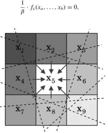
Figure 1 illustrates the basic idea of C-SART for a two-dimensional case (2D) in which there are nine cells (with values xj, j = 1,2, . . . ,9), and a ray never crosses the middle cell (x5). In this case, information about the value of the center cell can be transferred from the neighboring cells if a number of assumptions are made about the underlying field. Generally, any physically reasonable information, ex-pressed in the form of a finite difference equation, can be transferred. Treating the media as a smooth field—i.e., no steep gradients between neighboring cells—is a reasonable way to simplify the discussion and to enable this approach to be extended to applications other than ionosphere tomog-raphy. One way to do this is to use the 2D-Laplacian oper-ator,
which relates the values for the neighboring cells to that of the cell at the center. This operator is used to compute the difference between the sum of the values for the surround-ing cells and the value for the center cell, which is multi-plied by the number of neighboring cells. Since the mean value of all entries in the matrix is zero, application to the ionosphere does not bias the total number of electrons in the field. The operator has to be modified accordingly when the concerned cell lies on the edge of the model space. It can be used to introduce an artificial observation between un-knowns, a so-called “constraint”. Thus, it is possible to im-pose, for the nine-cell example, one constraint for each by applying the smoothness operator to the surrounding cells. This simple approach can be applied to any cell, indepen-dent of the number of crossing rays, to guarantee that the estimated field is smooth. This constraint, expressed as a function of fcin its general form, can be denoted as
1
β · fc(xa, . . . ,xb)=0, (11)
Fig. 1. Basic idea of C-SART for two dimensional (2D) case. The
xj(j = 1,2, . . . ,9)represent the cells, which are gray shaded on an
arbitrary scale. Cell at center (x5) is never crossed by a ray. Placement of a Laplacian constraint on the underlying field enables the value ofx5
to be deduced from those of neighbor cells.
wherexa, . . . ,xbincludes all of the unknowns related to the condition. Each constraint is weighted by hyper-parameter (weight parameter)β, which determines the extent to which the condition must be fulfilled. The choice of β should be cross-validated to ensure that the reconstructed field is neither too rough nor too smooth. Expressing the Laplace operator as a constraint yields
1
where C is the number of neighboring cells, which can range between 3 and 8 (for the 2D case) depending on the position of cell jin the grid. It is thus possible to set up one constraint for each cell that increases the number of obser-vations (by the number of cells) and makes the whole sys-tem overdetermined. For small grids, the solution can be easily obtained using traditional least-squares adjustment since redundancy is ensured by the constraints. Even for a 2D case of 100×100 cells, SART is much faster than the inversion of the corresponding 10,000×10,000 design ma-trix from the Gauss-Markov model. In general, heat-, wave-or Laplace-partial derivative equations can be expressed us-ing finite differences, and dedicated constraint operators, similar to expression 10, can be set up. Moreover, it is possible to support the estimates by considering physical relationships given as explicit equations. For the case of the ionosphere, it might be useful to constrain the solution to follow Chapman-like vertical profiles (as described, for example, by Hargreaves, 1992). Thus, it is possible to write
xj −xmexp 1−
wherexmis the electron density maximum andhmthe cor-responding height for each vertical profile. Operatorh(xj)
returns the height of cell j, and H is the scale height of a hydrostatic equilibrium (e.g., Hargreaves, 1992). To ap-ply this constraint within C-SART, it is necessary to com-putexmandhm from the results of the prior iteration step. In general, the Laplacian constraint could be used together with the Chapman profile approach if the user wants to force the resulting field to follow simple physical conditions of the ionosphere. For the tomographic inversion discussed in Section 4.2, such a Chapman constraint was not applied since our intention was to demonstrate that C-SART per-forms well even without knowledge of the underlying field. As discussed above, for the case in which DCBs have to be estimated together with the electron density field, it is com-mon to constrain the sum of the satellite DCBs to zero to achieve a virtual but stable reference (Schaer, 1999). One can express this zero-sum condition as
1
wherexd are the cells corresponding to the DCBs, andβD
3.2 Mathematical prerequisites
Equation (12) violates condition (6) since Ai,j < 0 is
possible. Moreover, when the coefficients of the imaging system take negative values, Ai,⊕ is negative. Therefore, the original SART had to be refined. Censor and Elfving (2002) showed that SART convergence is ensured when
Ai,⊕=
are used instead of Eqs. (3) and (4). Expression (2) does not need to be changed. The use of Eqs. (15) and (16) to compute Ai,⊕ and A⊕,j enables the C-SART algorithm to
be handled with the SART formalism described by Eq. (2).
4.
2D Reconstruction of Ionosphere Using
C-SART—A Test Case Using Artificial Data
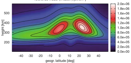
We used a 2D test scenario for testing the performance of the C-SART algorithm in comparison with the SART algo-rithm. One hundred ionosphere profiles were computed us-ing the international reference ionosphere (IRI) model (Bil-itza, 2001), version IRI2007. Data were obtained for the Greenwich meridian for latitudes between−49◦and 50◦for May 6, 2004, 1200 local time. The height ranged from 105 to 600 km in steps of 5 km, resulting in a grid of 100×100 electron density values (Fig. 2). This 2D electron density field was used as a reference for our investigation charac-terizing the quality of the tomographic inversion. Artifi-cial observations were assumed to be inside the plane of the profiles only, enabling us to treat the problem as a 2D one. Additionally, the curvature of the Earth was ignored to simplify the discussion. It was also assumed that the dispersive delays outside the model boundaries had been removed from each observation; this can be achieved with the help of theoretical models or simple approximations of the plasmasphere contribution (e.g., Maet al., 2005). For investigations including the plasmasphere and higher alti-tudes, it would be worthwhile adding a coarse voxel struc-ture above the ionosphere domain. The electron densities of these voxels can be obtained together with the ionosphere-related values from the same tomographic inversion.
To obtain a realistic, but weak spatial distribution of the receivers, we assumed that the ionosphere was probed by 14 ground receivers and two low Earth-orbiting (LEO) satellites, which provided occultation data. The number of GNSS satellites traceable by all receivers was set to six. Data from three arbitrary epochs were used to reconstruct the media (Fig. 3). This test geometry does not totally re-flect a real-word scenario since the GPS-to-ground geom-etry changes much less frequently than LEO occultations occur. Nevertheless, since our investigation focused on the improvement in the reconstructed electron density field due to usage of C-SART, we can draw conclusions from our results about how GNSS applications can benefit from C-SART. Once the algorithm has been implemented in a way that permits fast computation of dense 3D electron density
0.0e+00
reference model (IRI2007) [el./cm3]
-40 -30 -20 -10 0 10 20 30 40
Fig. 2. Reference ionosphere latitude profile generated from the IRI2007 model run assuming May 6, 2004, 1200 LT, at 0◦longitude. Obtained electron densities are referenced to the mid-point of each cell.
500
Fig. 3. Ray geometry obtained from 14 ground receivers and two LEO satellites, which provided occultation data. Six GNSS satellites were traceable by all receivers. Each receiver tracked satellites in three dif-ferent epochs, with angular separation between consecutive epochs of 1 degree.
fields, we plan to test it using data from dense ground GNSS receiver networks.
Slant total electron content values were obtained for each observation by ray-tracing through the reference iono-sphere, ignoring contributions from electrons at higher alti-tudes or outside the latitude boundaries. A total of 10,022 unknowns (including electron density values for the cells and the receiver and satellite DCBs) were estimated from 288 (= (14+2)·6·3) observations, which is a highly under-determined situation for tomographic inversion. Of the pixels, 11% were not hit by any ray, and 21.9% were hit by only one ray. Therefore, with traditional SART, many cells would need support from background models or would even be removed from the tomographic inversion. In total, about one-third of the field would lack good ray coverage and thus would not be reconstructed unbiased.
The DCB values for the receivers and satellites were added to the ray-traced STEC values to simulate actual GNSS conditions. The ambiguities were assumed to have already been resolved (e.g., Horvath and Crozie, 2007), so it was possible to treat the data like code-leveled phase measurements. The artificial measurements were corrupted with Gaussian random noise, at a signal-to-noise ratio (SNR) of 100, to obtain more realistic signal characteris-tics.
4.1 Optimum choice of constraint weights by model verification
cross-Fig. 4. Results of cross-validation test after 1,000,000 iterations for different values of constraint weightsβLandβD. Left plot shows results for
L2-space metric,ρL2; right plot shows them for c-space metric,ρc.
validated. Andreeva et al.(1992) proposed two measures for describing the deviation between two models. In one, the metric is assigned to the L2 space; in the other, it is assigned to the c-space. The first metric,
ρL2=
N
i=1
(xi˜ −xi)2
N
i=1 ˜
x2
i
, (17)
is the ratio between the standard deviations of the differ-ences and the original field valuesxi˜. Thus, a small value ofρL2 can be taken as an indicator of good global perfor-mance for tomographic inversion. The second metric,
ρc= max
i | ˜xi−xi|
max
i | ˜xi|
, (18)
utilizes local performance characteristics by relating the largest reconstruction error to the largest true value. The better the performance, the smaller the metric. Thus, to find the optimum constraint weight parametersβL andβD, we
computedρL2andρcfor different weights. Figure 4 shows the results of the cross-validation test after one million iter-ations for different values of the constraint weights. Agree-ment with the model strongly depended on the value set for βL, and agreement was best whenβL was set to one. The selection of theβDvalue was less critical as it did not have
a noticeable effect onρL2andρcas long asβL >0.1. Since βL strongly determines the roughness of the reconstructed field, setting of its value can lead to bigger reconstruction errors when the field is forced to be too smooth (βL <1). IfβL is set to a value larger than one, the algorithm cares less about the Laplacian constraints and tends to perform in a way similar to classical SART. Thus, in the following examples,βL = βD = 1 is used for the reconstruction of
the electron density field. For tomographic problems with a larger number of rays, a cross-validation test should be done again to determine an optimum pair of values forβL andβD
4.2 Tomographic reconstruction results for SART and C-SART
Using SART and C-SART with the optimum constraint weights from above, we reconstructed the electron density
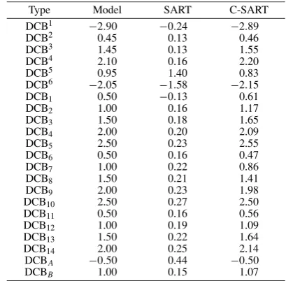
Table 1. Modeled and reconstructed (after 106iterations) DCB values for
SART and C-SART algorithms. DCBsrepresents value for GNSS satel-lites, and DCBr represents value for receiverr. Values for receivers
on-board LEO satellites are denoted byAandB.
Type Model SART C-SART
DCB1 −2.90 −0.24 −2.89
DCB2 0.45 0.13 0.46
DCB3 1.45 0.13 1.55
DCB4 2.10 0.16 2.20
DCB5 0.95 1.40 0.83
DCB6 −2.05 −1.58 −2.15
DCB1 0.50 −0.13 0.61
DCB2 1.00 0.16 1.17
DCB3 1.50 0.18 1.65
DCB4 2.00 0.20 2.09
DCB5 2.50 0.23 2.55
DCB6 0.50 0.16 0.47
DCB7 1.00 0.22 0.86
DCB8 1.50 0.21 1.41
DCB9 2.00 0.23 1.98
DCB10 2.50 0.27 2.50
DCB11 0.50 0.16 0.56
DCB12 1.00 0.19 1.09
DCB13 1.50 0.22 1.64
DCB14 2.00 0.25 2.14
DCBA −0.50 0.44 −0.50
DCBB 1.00 0.15 1.07
fields. One million iterations were carried out, withβDset
the same for both algorithms. Figure 5 shows the recon-structed fields for both algorithms. The classical SART al-gorithm did not reconstruct the model ionosphere well and even produced some negative electron density values. Since all unknowns were initialized with zero values, the cells not crossed by rays retained this value through all iterations. Moreover, the DCBs (Table 1) were not recovered at all, which directly translated into artifacts in the reconstructed image. In contrast, the C-SART algorithm reconstructed the model ionosphere much better. It did not produce neg-ative values, the recovered field looked very similar to the model one (Fig. 1), and the uncrossed cells were updated with information from the neighboring ones by the Lapla-cian constraint as expected. The absolute relative error of the C-SART reconstruction, as depicted in Fig. 6, did not exceed 75% and was less than 15% for most of the regions. Closer examination revealed that the areas with higher rel-ative errors had lower electron densities, meaning that their absolute reconstruction error was not necessarily large.
im-Fig. 5. Reconstructed electron density fields after 1,000,000 iterations. Left figure shows estimated field for SART, and right one shows it for C-SART. Note that the range of the values differs between plots and that color coding is not the same.
Fig. 6. Absolute relative reconstruction errors with respect to IRI model for SART (left) and C-SART (right) algorithms. Note that the range of the values differs between plots and that color coding is not the same.
Fig. 7. Electron density fields reconstructed by SART and C-SART when DCBs were known and models were initialized with IRI2007 data from an epoch 1 month earlier. Upper plots show reconstructed fields, and lower plots show corresponding absolute relative errors with respect to original field.
age produced a mean reconstruction error of 11.9%, which is in good agreement withρL2, a similar measure. The ab-solute relative errors for the SART reconstruction (Fig. 6) were large (82% on average). This clearly demonstrates that C-SART provides much better results than SART.
4.2.1 Reconstruction of differential code biases
Satellite DCBs are usually known up to a certain accuracy level since they are monitored on a daily base by several GNSS analysis centers (Feltens, 2003). The receiver biases
million iterations. C-SART clearly reconstructed the satel-lite and receiver biases, whereas classical SART did not. The zero-sum constraint, applied to the satellite DCBs, was met in both cases, but only C-SART with its simple Lapla-cian constraints on the electron density field produced the values correctly. Since SART did not iterate towards the correct satellite DCBs, the receiver DCBs and the electron density field itself were negatively affected. The satellite DCBs from C-SART were within 0.17 TECU (total elec-tron content) of the model values. Those for the ground-based and LEO on-board receivers were within about the same range. These estimated DCB values should satisfy user needs, especially when the low number of input obser-vations and the weak observation geometry are considered. The values from SART did not agree with the model ones, negatively affecting reconstruction of the electron density field.
4.2.2 Known DCBs and initialization with
back-ground model To demonstrate how SART and C-SART
perform when all DCBs are known and the models are ini-tialized with a background ionosphere model, IRI2007 elec-tron density profiles were computed for an epoch of 1 month preceding the one used in the previous section. This was done to ensure that the cells were initialized with values that were realistic but also sufficiently different considering that the background model has a limited ability to predict actual conditions. As the receiver and satellite DCBs were known, only the electron density values for each cell had to be estimated. Nevertheless, SART did not update the uncrossed cells, and the values of the background model remained unchanged. Thus, the quality of the background model strongly determines the accuracy with which SART can recover the ionosphere when the geometrical coverage is poor.
The electron density fields reconstructed by the SART and C-SART algorithms are shown in Fig. 7 together with the absolute relative errors. The performance of SART was greatly improved: the average absolute reconstruction error was 16.1%, and the maximum was 235%. The C-SART al-gorithm benefited only slightly from the background model initialization: the mean absolute relative reconstruction er-ror improved slightly to 11.6%. However, the field recon-structed by C-SART was slightly degraded in the upper ionosphere (the maximum error in that region was 98.1%). Therefore, the use of a background model is significantly useful for the SART algorithm, but using it still does not solve the problem of uncrossed cells. The C-SART algo-rithm performs about 50% better than the SART one re-gardless of whether there is knowledge of the DCBs or the background model is initialized. The only advantage gained from using the background model for the C-SART algo-rithm is that the convergence speed is slightly faster, as dis-cussed in the next section.
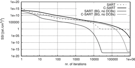
4.2.3 Convergence and computation speed The
sum of the squared improvements (SSI) for iterationk,
SSI=
Fig. 8. Convergence of SART (dashed line) and C-SART (thick line) measured using sum of squared improvements for each iteration step. The thick dotted lines correspond to SART and C-SART runs with known DCBs and background field initialization.
was used as an indicator of the convergence speed. Equa-tion (19) is also related to the energy (Maillouxet al., 1993) remaining in the system after the k-th iteration. Thus, it can be used to define a threshold for stopping the itera-tive process if SSI decreases to a certain value. Figure 8 plots SSI against the number of iterations for the SART and C-SART algorithms with and without DCB informa-tion and background model initializainforma-tion. When the DCBs were known and the background model was initialized, SSI stabilized before one million iterations for both algorithms. However, when the DCBs were estimated and the models were initialized with zero values, the SSI for SART did not decrease much, and that for C-SART saturated only after about 1.2 million iterations (not shown here). For practical applications, it is sufficient to stop the iterations once SSI drops below 10−2(electrons2/cm6) as any subse-quent improvements are usually too small to affect the to-mography results. It took 737 s to complete 106iterations with SART and 1418 s with C-SART. C-SART reached the threshold of 10−2 (electrons2/cm6) in about 2·105 itera-tions. Thus, it took only 4 min and 44 s (i.e., 284 s) on a simple PC (2.3-GHz Pentium D CPU, 2-GB RAM) to carry out high-resolution ionospheric tomography and esti-mate the unknown DCB values (although their values might have stabilized in an earlier iteration). The coding of the C-SART algorithm in a low-level programming language will lead a significant reduction in computing time (by at least an order of magnitude).
5.
Discussion
Our simple algorithm, the constrained simultaneous alge-braic reconstruction technique (C-SART), has many advan-tages for reconstructing the ionosphere by means of elec-tron density values using GNSS measurements. It is suit-able for real-time applications and even ensuit-ables estimation of instrumental biases within a reasonable processing time. The reconstructed fields are significantly better than those obtained from classic SART. Moreover, C-SART can esti-mate the DCB values accurately enough when necessary.
for an unbiased reconstruction of the ionosphere. Since C-SART is based only on the assumption that the under-lying field is smooth, it can be applied to other tomography applications as well. It is also easy to apply other condi-tions in the form of difference equacondi-tions to the algorithm, e.g., heat-, wave-, and Laplace-partial derivative equations. This means that physical conditions estimated from mea-surement data can be considered in the field reconstruction, resulting in better representation (including unprobed areas) of the media. One drawback of the smoothness operator is that, for applications in which the media contain disconti-nuities, the C-SART algorithm gives incorrect results. In the case of steep gradients, the grid should be refined or βLshould be increased in order to allow for more variation between cells.
6.
Future Work
To enable the C-SART algorithm to be used for (near) real-time 3D tomography of the ionosphere, we need to speed it up by a factor of 100 or more. Assuming that GNSS observations are taken every 30 s and that some time is spent on data transfer and the leveling of the L1– L2 phase measurements, about 15 s should remain for iono-spheric reconstruction. A speed-up by a factor of 10 or can be achieved by optimizing the routines and loops and by coding parts of the algorithm in a low-level programming language (e.g., Assembler). In addition, the reconstruction could be modularized using either message parsing inter-faces (described, for example, by Skjellumet al., 1993) or OpenMPTM(Dagum and Menon, 1998), which distributes the computation load among multi-core processors.
The C-SART algorithm can thus be speeded up (nearly) proportional to the number of core processors used. More-over, Moore’s Law (Moore, 1965), which predicts the num-ber of transistors in future CPUs, indicates that the re-alization of on-line monitoring of the ionosphere using C-SART is feasible. Additionally, a large number of iter-ations (2·105) is not necessary when models are gener-ated in 30-s intervals since each model run can be initialized with the results of the prior one, which will not differ much from the new one. Moreover, other measurements, such as ionosonde profiles, can be utilized when available.
Although C-SART has been applied to ionosphere to-mography it is not necessarily limited to this single applica-tion. Basically, it can be used for any kind of tomographic inversion as long as constraints can be defined in a mean-ingful sense. For example, C-SART can be used for seis-mic prospection by applying a-priori velocity information as constraints. It can be used for other problem statements occurring in seismology, atmosphere, space-physics, and medical research without any large modifications. Thus, the flexibility of C-SART, paired with increasing computational power, will make it a powerful tool for a variety of scientific applications.
Acknowledgments. We are very grateful to the Japanese Society for the Promotion of Science, JSPS for supporting our research (project P06603, “Study on the improvement of accuracy in space geodesy”). The two anonymous reviewers are acknowledged for the valuable comments that led to significant improvements in our report.
References
Andersen, A. H. and A. C. Kak, Simultaneous algebraic reconstruction technique (SART): a superior implementation of the ART algorithm,
Ultrason. Img.,6, 81–94, 1984.
Andreeva, E. S., V. E. Kunitsyn, and E. D. Tereshchenko, Phase-difference radio tomography of the ionosphere,Ann. Geophys.,10, 849–855, 1992. Bhuyan, K., S. B. Singh, and P. K. Bhuyan, Application of generalized sin-gular value decomposition to ionospheric tomography,Ann. Geophys., 22, 3437–3444, 2004.
Bilitza, D., International Reference Ionosphere 2000,Radio Sci.,36(2), 261–275, 2001.
Censor, Y. and T. Elfving, Block-iterative algorithms with diagonally scaled oblique projections for the linear feasibility problem,SIAM J. Matrix Anal. Appl.,24, 40–58, 2002.
Dagum, L. and R. Menon, OpenMP: an industry-standard API for shared-memory programming,IEEE Comput. Sci. Eng.,5(1), 46–55, 1998. Feltens, J., The activities of the ionosphere working group of the
Inter-national GPS Service (IGS),GPS Solutions,7(1), 41–46, doi:0.1007/ s10291-003-0051-9, 2003.
Gordon, R., R. Bender, and G. T. Herman, Algebraic reconstruction tech-niques (ART) for three-dimensional electron microscopy and X-ray photography,J. Theor. Biol.,29, 471–482, 1970.
Hajj, G. A., B. D. Wilson, C. Wang, X. Pi, and I. G. Rosen, Data assimilation of ground GPS total electron content into a physics-based ionospheric model by use of the Kalman filter,Radio Sci.,39, doi:10.1029/2002RS002859, 2004.
Hansen, P. C., The truncated SVD as a method for regularization,BIT,27, 534–553, 1987.
Hargreaves, J. K., Thesolar-terrestrial environment, Cambridge Univer-sity Press, Cambridge, 1992.
Hernandez-Pajares, M., J. M. Juan, and J. Sanz, New approaches in global ionospheric determination using ground GPS data,J. Atmos. Solar Terr. Phys.,61, 1237–1247, 1999.
Horvath, I. and S. Crozie, Software developed for obtaining GPS-derived total electron content values, Radio Sci., 42, RS2002, doi:10.1029/ 2006RS003452, 2007.
Ivansson, S., Seismic borehole tomography—theory and computational methods,Proc. IEEE,76(2), 328–338, 1986.
Jiang, M. and G. Wang, Convergence of the simultaneous algebraic recon-struction technique (SART),IEEE Trans. Image Proc.,12(8), 957–961, 2003.
Kalman, R. E., A new approach to linear filtering and prediction problems,
Trans. ASME—J. Basic Eng.,82(D), 35–45, 1960.
Koch, K. R.,Parameter estimation and hypothesis testing in linear models, Springer, Berlin, 1988.
Lee, J. K., F. Kamalabadi, and J. J. Makela, Localized three-dimensional ionospheric tomography with GPS ground receiver measurements, Ra-dio Sci.,42, RS4018, doi:10.1029/2006RS003543, 2007.
Ma, X. F., T. Murayama, G. Ma, and T. Takeda, Three-dimensional iono-spheric tomography using observation data of GPS ground receivers and ionosonde by neural network, J. Geophys. Res.,110, A05308, doi:10.1029/2004JA010797, 2005.
Mailloux, G. E., R. Noumeir, and R. Lemieux, Deriving the multiplicative algebraic reconstruction algorithm (MART) by the method of convex projections (POCS),Proc. IEEE Int. Conf. Acoustics, Speech Signal Proc.,5, 457–460, 1993.
Moore, G. E, Cramming more components onto integrated circuits, Elec-tronics,38, 114–117, 1965.
Ray, J. and K. Senior, Geodetic techniques for time and frequency compar-isons using GPS phase and code measurements,Metrologia,42, 215– 232, 2005.
Raymund, T. D., Comparison of several ionospheric tomography algo-rithms,Ann. Geophys.,13, 1254 –1262, 1995.
Ruffini, G. A. Flores, and A. Rius, GPS tomography of the ionospheric electron content with a correlation functional,IEEE Trans. Geosci. Re-mote Sens.,36(1), 143–153, 1998.
Schaer, S., Mapping and predicting the Earth’s ionosphere using the Global Positioning System, PhD thesis, Astronomical Institute, University of Bern, 1999.
Skjellum, A., N. E. Doss, and P. V. Bangalore, Writing libraries in MPI.
Proceedings of the Scalable Parallel Libraries Conference, IEEE Com-puter Society Press, 166–173, 1993.
Wen, D. B., Imaging the ionospheric electron density using a combined to-mographic algorithm,Proceedings of the International Technique Meet-ing of the Satellite Devision, 25–28 September 2007, Fort Worth, Texas, 2337–2345, 2007.
Wen, D. B., Y. B. Yuan, J. K. Ou, and X. L. Huo, Monitoring the three-dimensional ionospheric electron distribution using GPS observations over China,J. Earth Syst. Sci.,116(3), 235–244, 2007a.
Wen, D. B., Y. B. Yuan, J. K Ou., X. L. Huo, and K. F. Zhang,
Three-dimensional ionospheric tomography by an improved algebraic recon-struction technique,GPS Solutions,11(4), 251–258, 2007b.
Wen, D. B., Y. B. Yuan, J. K Ou., X. L. Huo, and K. F. Zhang, Ionospheric temporal and spatial variations during the 18 August 2003 storm over China,Earth Planets Space,59, 313–317, 2007c.