R E S E A R C H
Open Access
Approximate solution of linear Volterra
integro-differential equation by using cubic
B-spline finite element method in the
complex plane
M. Erfanian
1*and H. Zeidabadi
2*Correspondence: [email protected]
1Department of Science, School of Mathematical Sciences, University of Zabol, Zabol, Iran
Full list of author information is available at the end of the article
Abstract
So far, there are no any publications for solving and obtaining a numerical solution of Volterra integro-differential equations in the complex plane by using the finite element method. In this work, we use the linear B-spline finite element method (LBS-FEM) and cubic B-spline finite element method (CBS-FEM) for solving this equation in the complex plane. We also discuss the error and convergence of the method. Furthermore, we give some numerical examples to substantiate efficiency of the proposed method.
Keywords: Complex linear Volterra integro-differential equation; Finite element method; Error estimation
1 Introduction
One of the first works in imaginary numbers was by the Persian mathematician Al-Khwarizmi. However, the first person who used them is Girolamo Cardano (1501–1576). Also, Paul Nahin gave a detailed description of imaginary numbers [1]. The symboli in-stead of√–1 was proposed by Euler (1707–1783). The interpretation of complex numbers as points in the plane was suggested by Carl Friedrich Gauss (1777–1855). Gauss also demonstrated that every polynomial equation of degreenwith nonzero complex coeffi-cients hasnroots in complex numbers. The complex functions and their integrals were studied by Gauss and Simon Denis Poisson (1781–1840). August Louis Cauchy (1789– 1857) published a large number of researches on the integral theorem and related con-cepts. George Bernhard Riemann (1826–1860) introduced the derivatives of functions of complex variables [2].
The complex numbers and functions have unbelievable properties, which are used to solve science and engineering problems such as contour integration, electrical engineer-ing, digital filters, generating functions, physical problems, Fourier analysis, conformal mappings, mechanical problems, eigenvalues, and mechanical systems. Also, they are used in phasor transforms to analyze networks composed of resistors, capacitors, and induc-tors. For instance, in digital signal processing, complex Fourier, Laplace, and z-transforms are used; see [3].
We can solve integro-differential equations with some basis functions by the Haar and rationalized function methods [4–8], Adomian decomposition method [9], Legen-dre wavelets method [10], RBFs collocation method [11], and Genocchi polynomials and collocation method based on the Bernoulli operational matrix [12, 13]. Also, in [14], Volterra–Fredholm integro-differential equations of fractional order are solved by the sinc-collocation method.
So far, there are no any publications in the field of integro-differential equations in the complex plane by the finite element method. Recently, some work has been done by the rationalized Haar function method [15–17] and by the collocation method based on the Bernoulli operational [18].
Spline functions are a class of piecewise polynomials that satisfy continuity proper-ties depending on the degree of the polynomials. They have highly desirable characteris-tics, which have made them a powerful mathematical tool for numerical approximations. Spline functions are a set of continuous combinations of B-splines used as trial functions in the Galerkin method [19–23].
This work is organized as follows. In Sect.2, we use the of the finite element method, especially, the linear B-spline finite element method (LBS-FEM) and cubic B-spline finite element method (CBS-FEM) [19] to obtain an approximate solution of a linear Volterra integro-differential equation in the complex plane. The convergence analysis is given in Sect.3, and numerical experiments are carried out in Sect.4to verify the theoretical re-sults.
2 The proposed method
We consider the linear second-order Volterra integro-differential equations of the second kind in complex plane with boundary conditionsu(0) = 0 andu(1) = 0:
–u(x) +b(x)u(x) +c(x)u(x) =f(x) +i x
0
K(x,t)u(t)dt, x∈[0, 1], (1)
where u(x) is an unknown complex-valued function to be determined, and f(x) is a complex-valued function; in other words,
u: [0, 1]⊆R→C f: [0, 1]⊆R→C
u(x) =u1(x) +iu2(x), f(x) =f1(x) +if2(x), u1,u2∈C2
[0, 1], f1,f2∈C
[0, 1].
(2)
Moreover,b(x) andc(x) are nonnegative functions belonging toC1([0, 1]), andK(x,t) is a
known continuous function on [0, 1]×[0, 1]. Using (2) in (1), we have
–u1(x) +b(x)u1(x) +c(x)u1(x) =f1(x) –
x
0
K(x,t)u2(t)dt,
–u2(x) +b(x)u2(x) +c(x)u2(x) =f2(x) +
x
0
K(x,t)u1(t)dt.
(3)
Ifπ: 0 =x0<x1<· · ·<xM= 1 is a grid withM+ 1 points in the interval [0, 1], where upon an increasing set ofM+ 1 knots over the problem domain plus six additional knots outside the problem as
0 in the other nodes,
and thusQ2,Q3, . . . ,QM–2 satisfy the zero boundary conditions, butQ–1,Q0,Q1,QM–1, QM, andQM+1do not. Therefore we modify cubic B-spline basis functions for handling
variational form of equation (1). SetΩ = [0, 1]⊂R. First, we define V =H1
0(Ω) as an
infinite-dimensional space andB:V×V→Ras a bilinear form. So we have
B(u,v) =
The spaceVis infinite-dimensional, and thus we introduce a finite-dimensional subspace
VhofV. So the problem is converted to finduh= (u1,h,u2,h)∈Vhsuch that
Hence by substituting (5) into the variational formulation we have
andCin the 2(M– 1)×2(M– 1)-dimensional matrix given by
In this section, we present the error analysis theorems for the proposed method. For this purpose, letVbe a Hilbert space, and letBbe a symmetricV-elliptic bilinear form. Then the inner product energy is (·,·) :V×V→Rdefined by (u,v)B=B(u,v). Additionally, the energy norm is
u2
E= (u,u)B.
Definition 3.1 For an operatorΠ:V→Vh, the projection operators are defined as
Πu=u˜h=
Using the Cauchy–Schwarz inequality and Sobolev norm, we have
B(u,v)≤ uH1vH1+P2uH1vH1+M2uH1vH1+KRuH1vH1
whereC= (1 +P2+M2+KR),K=max|K(x,t)|,x∈[0, 1],t∈[0,x], andR=12L2(Ω). Thus Bis continuous. Furthermore, we prove theV-ellipticity ofB. For this purpose, we have
Therefore, by the Lax–Milgram theorem and the V-ellipticity ofB, equation (1) has a unique solution. Suppose thatuhis an approximate solution. Then we have
B(u,vh) =L(vh) ∀vh∈Vh (15)
and
B(uh,vh) =L(vh) ∀vh∈Vh. (16)
Ife=u–uh, whereuis an exact solution of (1), then
B(e,vh) = 0 ∀vh∈Vh. (17)
By the relation between the inner product and energy norm, using the Schwarz inequality, we have
B(v,w)≤ vEwE ∀v,w∈V. (18)
Since (e,vh)B=B(e,vh) = 0, (17) yields thateis orthogonal to anyvh. Also, for each partic-ularv˜hinVh,u–uhE=min{u–vhE;vh∈Vh}, and using Cea’s lemma [24], we have
ifv˜his equal tou˜h, and we get an upper bound for the interpolation error. Also,
u–uhV≤cu–u˜hV≤cMhζ, ζ> 0,
where the constantcis independent ofh. Therefore
u–uhV≤ CM
η h ζ
.
Hence the norm of error tends to zero ash→0, and the order of the method isO(hζ).
4 Results and discussion
In this section, we solve two numerical examples with the proposed methods. In addition, we compare exact and numerical solutions of examples obtained by CBS-FEM and LBS-FEM forM= 10 andh=M1. Also, we present an algorithm on the basis of our discussions to solve Volterra integro-differential equations in the complex plane.
• Algorithm:
Step 1. ChooseMcollocation points in the finite domainΩ= [0, 1]; Step 2. Corresponding to each node, construct a basis function{φi}Mi=1. Step 3. Compute the vectorFand the matrixCby (8) and (9), respectively. Step 4. Compute the coefficientsαiandβiby solving system (7).
Step 5. Compute the approximate solutionuhfrom equation (5).
Also, we show the ability and effectiveness of our method by obtaining the absolute error for the modules ofu(x) as
|error|=(Reu–Reuh)2+ (Imu–Imuh)2.
All the solutions are obtained by using symbolic computation software Maple 16 on a machine with Intel Core i5 Duo processor 2.6 GHz and 4 GB RAM.
Example4.1 Consider the following linear complex Volterra integro-differential equation:
–u(x) +u(x) + 2u(x) =f(x) +i x
0
xtu(t)dt, 0 <x≤1,
wheref(x) =f1(x) +if2(x), and
f1(x) = –11cos(3x) + 1 +cos(3) + 3sin(3x) – 2
1 –cos(3)x
+ 1
12x
4sin(2)x3+ 6cos(2x)x– 3sin(2x),
f2(x) = –6sin(2x) +sin(2) – 2cos(2x) – 2
1 –sin(2)x+17x 9
–1 3cos(3)x
4+1
3x
4+1
3sin(3x)x
2–1
2x
3+1
9cos(3x)x.
At first, transformation formulas should be used to convert the inhomogeneous bound-ary conditions to homogeneous boundbound-ary conditions. Diagrams of exact and numerical solutions and the graph of error for Example4.1with the cubic B-spline finite element method is showed in Fig.1. Also, the comparison between exact and numerical solutions forM= 10 andM= 20 in Example4.1are presented in Tables1and2, respectively.
Figure 1Diagrams of exact and numerical solutions and graph of error for modules of Example4.1with cubic B-spline finite element method forM= 10
Table 1 Comparison of exact and numerical solutions for Example4.1
x exact solution CBS-FEM LBS-FEM error(CBS-FEM) error(LBS-FEM)
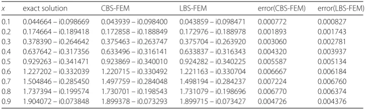
0.1 0.044664 – i0.098669 0.042820 – i0.098403 0.044050 – i0.098687 0.001863 0.000061 0.2 0.174664 – i0.189418 0.173427 – i0.188851 0.173440 – i0.189375 0.001361 0.001225 0.3 0.378390 – i0.264642 0.375337 – i0.263756 0.376476 – i0.264457 0.003179 0.001923 0.4 0.637642 – i0.317356 0.633653 – i0.316139 0.634900 – i0.316972 0.004171 0.002768 0.5 0.929263 – i0.341471 0.923961 – i0.340041 0.925567 – i0.340893 0.005491 0.003741 0.6 1.227202 – i0.332039 1.220711 – i0.330465 1.222553 – i0.331356 0.006679 0.004699 0.7 1.504846 – i0.285450 1.498093 – i0.284178 1.499533 – i0.284814 0.006872 0.005351 0.8 1.737394 – i0.199574 1.730275 – i0.198350 1.732179 – i0.199139 0.007223 0.005232 0.9 1.904072 – i0.073848 1.900770 – i0.073877 1.900372 – i0.073677 0.003302 0.003704
Table 2 Comparison of exact and numerical solutions for Example4.1,M= 20
x exact solution CBS-FEM LBS-FEM error(CBS-FEM) error(LBS-FEM)
Example4.2 In this example, we consider the following linear Volterra integro-differential equation:
–u(x) +sin(x)u(x) +xu(x) =f(x) +i x
0
(x–t)u(t)dt, 0 <x≤1,
wheref(x) =f1(x) +if2(x) and
f1(x) =
1 12
(–6x+ 4)sinh(1) + 3e–1+ e(x– 1)sin(1)
+ 1
12
–12x2– 12sin(x)sinh(1) + (3x– 6)e–1– 3xecos(1)
+ 1
12
12xcos(x) + 12cos(x)2– 12sinh(x)
+sin(x)cosh(x)cos(x) + 2sin(x)cosh(x) +1 2,
f2(x) =
1 12
(6x– 4)sinh(1) – 3e–1+ e(x– 1)cos(1)
+ 1
12
–12x2– 12sin(x)sinh(1) + (3x– 6)e–1– 3xesin(1)
+ 1
12
–12cos(x)2– 24cos(x) + 12cosh(x)
+sin(x)sinh(x)x+sin(x)sinh(x)cos(x) +x 2.
The exact solution isu(x) =cos(x)sinh(x) +i(sin(x)sinh(x)).
ForM= 10 andM= 20, the results obtained by using CBS-FEM and LBS-FEM are pre-sented in Tables3and4and Fig.3.
5 Conclusions
In this work, we used the linear spline finite element method (LBS-FEM) and cubic B-spline finite element method (CBS-FEM) for solving and obtaining numerical solutions of Volterra integro-differential equations in the complex plane. So far, there are no any publications in this field in the complex plane by using the finite element method. The main purpose of this paper is to use the finite element method to find an approximate solution of (1). To this end, we must obtain a weak and variational form of equation (1). Also, the error and convergence of the method are discussed. The order of convergence
Table 3 Comparison of exact and numerical solutions for Example4.2
x exact solution CBS-FEM LBS-FEM error(CBS-FEM) error(LBS-FEM)
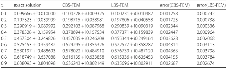
Table 4 Comparison of exact and numerical solutions for Example4.2,M= 20
x exact solution CBS-FEM LBS-FEM error(CBS-FEM) error(LBS-FEM)
0.1 0.099666 + i0.010000 0.100291 + i0.009703 0.100194 + i0.010499 0.000691 0.000726 0.2 0.197323 + i0.039999 0.197895 + i0.039802 0.197735 + i0.040591 0.000605 0.000721 0.3 0.290919 + i0.089992 0.290960 + i0.089624 0.390736 + i0.090365 0.000369 0.000416 0.4 0.378328 + i0.159954 0.377536 + i0.159159 0.377240 + i0.159896 0.001121 0.001089 0.5 0.457304 + i0.249826 0.455567 + i0.248503 0.455192 + i0.249227 0.002182 0.002195 0.6 0.525453 + i0.359482 0.522883 + i0.357628 0.522414 + i0.358351 0.003167 0.003242 0.7 0.580197 + i0.488693 0.577145 + i0.486461 0.576579 + i0.487178 0.003780 0.003921 0.8 0.618749 + i0.637088 0.615928 + i0.634747 0.615200 + i0.635499 0.003665 0.003888 0.9 0.638093 + i0.804098 0.636498 + i0.802167 0.635610 + i0.802937 0.002503 0.002740
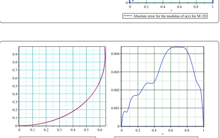
Figure 2Diagrams of exact and numerical solutions and graph of error for modules of Example4.1with cubic B-spline finite element method forM= 20
Figure 3Diagrams of exact and numerical solutions and graph of error for modules of Example4.2with cubic B-spline finite element method forM= 10
is computed, and we showed that it isO(hζ). Furthermore, the efficiency of the proposed
Figure 4Diagrams of exact and numerical solutions and graph of error for modules of Example4.2with cubic B-spline finite element method forM= 20
Acknowledgements
The authors would like to express their gratitude to the anonymous referees for their helpful comments and suggestions, which have greatly improved the paper.
Funding
We have no any fund. Competing interests
The authors declare that they have no competing interests. Authors’ contributions
Both authors read and approved the final version of the manuscript. Author details
1Department of Science, School of Mathematical Sciences, University of Zabol, Zabol, Iran.2Faculty of Engineering,
Sabzevar University of New Technology, Sabzevar, Iran.
Publisher’s Note
Springer Nature remains neutral with regard to jurisdictional claims in published maps and institutional affiliations.
Received: 16 October 2018 Accepted: 7 February 2019
References
1. Nahin, P.: The Story of√–1. Princeton University Press, Princeton (1998)
2. Burton, D.M.: The History of Mathematics. McGraw-Hill, New York (1995). ISBN 978-0-07-009465-9
3. Steven, W.S.: The Scientist and Engineer’s Guide to Digital Signal Processing (1999). California Technical Publishing ISBN 0-9660176-7-6
4. Lepik, Ü.: Haar wavelet method for nonlinear integro-differential equations. Appl. Math. Comput.176, 324–333 (2006) 5. Lepik, Ü.: Application of the Haar wavelet transform to solving integral and differential equations. Proc. Est. Acad. Sci.,
Phys. Math.56, 28–46 (2007)
6. Lepik, Ü., Tamme, E.: Solution of nonlinear Fredholm integral equations via the Haar wavelet method. Proc. Est. Acad. Sci., Phys. Math.56, 17–27 (2007)
7. Erfanian, M., Gachpazan, M., Beiglo, M.: A new sequential approach for solving the integro-differential equation via Haar wavelet bases. Comput. Math. Math. Phys.57(2), 297–305 (2017)
8. Erfanian, M., Gachpazan, M., Beiglo, M.: Rationalized Haar wavelet bases to approximate solution of nonlinear Fredholm integral equations with error analysis. Appl. Math. Comput.256, 304–312 (2015)
9. Wazwaz, A.M.: The combined Laplace transform–Adomian decomposition method for handling nonlinear Volterra integro-differential equations. Appl. Math. Comput.216, 1304–1309 (2010)
10. Yousefi, S., Razzaghi, M.: Legendre wavelets method for the nonlinear Volterra–Fredholm integral equations. Math. Comput. Simul.70, 1–8 (2005)
11. Jafari, M.A., Aminataei, A.: Application of RBFs collocation method for solving integral equations. J. Interdiscip. Math.
14(1), 57–66 (2011)
12. Loh, J.R., Phang, C., Isah, A.: New operational matrix via Genocchi polynomials for solving Fredholm–Volterra fractional integro-differential equations. Adv. Math. Phys.2017, Article ID 3821870 (2017)
13. Jalilian, Y., Ghasemi, M.: On the solutions of a nonlinear fractional integro-differential equation of pantograph type. Mediterr. J. Math.14(5), 194 (2017)
15. Erfanian, M., Zeidabadi, H.: Solving of nonlinear Fredholm integro-differential equation in a complex plane with rationalized Haar wavelet bases. Asian-Eur. J. Math.12(1), 1950055 (2019).
https://doi.org/10.1142/S1793557119500554
16. Erfanian, M.: The approximate solution of nonlinear mixed Volterra–Fredholm–Hammerstein integral equations with RH wavelet bases in a complex plane. Math. Methods Appl. Sci.41(18), 8942–8952 (2018)
17. Erfanian, M.: The approximate solution of nonlinear integral equations with the RH wavelet bases in a complex plane. Int. J. Appl. Comput. Math.4(1), 31 (2018).https://doi.org/10.1007/s40819-017-0465-7
18. Toutounian, F., Tohidi, E., Shateyi, S.: A collocation method based on the Bernoulli operational matrix for solving high-order linear complex differential equations in a rectangular domain. Abstr. Appl. Anal.2013, Article ID 823098 (2013)
19. Pourgholi, R., Tabasi, S.H., Zeidabadi, H.: Numerical techniques for solving system of nonlinear inverse problem. Eng. Comput.34, 487–502 (2018)
20. Dhawan, S., Kapoor, S., Kumar, S.: Numerical method for advection diffusion equation using FEM and B-splines. J. Comput. Sci.3, 429–437 (2012)
21. Ozis, T., Esen, A., Kutluay, S.: Numerical solution of Burgers equation by quadratic B-spline finite elements. Appl. Math. Comput.165, 237–249 (2005)
22. Ronglin, L., Guangzheng, N., Jihui, Y.: B-spline finite element method in polar coordinates. Finite Elem. Anal. Des.28, 337–346 (1998)
23. Sharma, D., Jiwari, R., Kumar, S.: Numerical solution of two point boundary value problems using Galerkin-finite element method. Int. J. Nonlinear Sci.13, 204–210 (2012)