Predetermined path of mobile data gathering in wireless sensor networks based on network layout

(1)

R E S E A R C H

Open Access

Predetermined path of mobile data gathering

in wireless sensor networks based on network

layout

Mukhtar Ghaleb

1

, Shamala Subramaniam

1,2*

, Mohamed Othman

1

and Zuriati Zukarnain

1

Abstract

Data gathering is among the issues constantly acquiring attention in the area of wireless sensor networks (WSNs). There is a consistent increase in the research directed on the gains of applying mobile elements (MEs) to collect data from sensors, especially those oriented to power issues. There are two prevailing strategies used to collect data in sensor networks. The first approach requires data packets to be serviced via multi-hop relay to reach the respective base station (BS). Thus, sensors will send their packets through other intermediate sensors. However, this strategy has proven to consume high and a substantial amount of energy due to the dependency on other nodes for transmission. The second approach encompasses a ME which serves as the core element for the searching of data. This ME will visit the transmission range of each sensor to upload its data before eventually returning to the BS to complete the data transmission. This approach has proven to reduce the energy consumption substantially as compared to the

multi-hop strategy. However, it has a trade-off which is the increase of delay incurred and is constrained by the speed of ME. Furthermore, some sensors may lose their data due to overflow while waiting for the ME. In this paper, it is proposed that by strategically divisioning the area of data collection, the optimization of the ME can be elevated. These derived area divisions are focused on the determination of a common configuration range and the correlation with a redundant area within an identified area. Thus, within each of these divided areas, the multi-hop collection is deployed as a sub-set to the main collection. The ME will select a centroid point between two sub-polling points, subsequently selecting common turning points as the core of the basis of the tour path. Extensive discrete-event simulations have been developed to assess the performance of the proposed algorithm. The acquired results depicted through the performance metrics of tour length and latency have determined the superior performance of the proposed algorithm in comparison to the existing strategy. In addition, the proposed algorithm maintains the energy consumption within an acceptable level.

Keywords: Wireless sensor networks; Mobile data gathering; Relay hop count; Polling points; Turning points; Mobile tour path

*Correspondence: Shamala_ks@upm.edu.my

1Department of Communication Technology and Network, Faculty of Computer Science and Information Technology, Universiti Putra Malaysia UPM, Serdang, Selangor 43400, Malaysia

2Sports Academy, Universiti Putra Malaysia UPM, Serdang, Selangor 43400, Malaysia

(2)

1 Introduction

Wireless sensor networks (WSNs) have gained substan-tial and critical attention over the last few years due to their impact and ability to transform many areas associ-ated with the human life. WSNs consist of hundreds or even thousands of sensors which are tiny, are low pow-ered and have limited storage and transmission. These sensors are used to acquire data that generally pose a chal-lenge or threat to humans in terms of accessibility and safety. Once the sensors are deployed, they are indeed unreachable due to their placement in hazardous envi-ronments such as in a volcano or tornado. In addition, these sensors which are powered by a battery have finite energy. Thus, factors such as inaccessibility to replenish power and constrained power supply have made energy consumption one of the primary issues in sensor net-works. Data transmissions and aggregation constitute a major portion of sensor energy consumption [1]. There is a rich and a heterogeneous spectrum of solutions to maximize the network lifetime. The related strategies are classified based on the type of data carrier which can be divided into two methods, the first being static (multi-hop) and the second being mobile. The static method focuses on routing using cooperative static sensor nodes. In this scheme, data packets are forwarded to the base station (BS) via multi-hop relay among sensors [2-12]. Strategies involving load balancing [2,3], spatio-temporal data [4,5], wake-up scheduling [6], energy balance [7-9], time synchronization [10] and cluster-based routing [12] have been extensively analysed and used to complement routing to further improve energy efficiency. Substantial energy is needed for the transmission or receiving of data. This is largely increased by the need of data forwarding along the path, especially for nodes which are located near the BS. These nodes serve as intermediate nodes, which cater the transmission needs of many other nodes. The deployment of the shortest path solution has not been able to prolong the network lifetime [1]. This is because some sensors may serve as intermediate nodes for many paths due to their unique positions, thus causing the depletion of their energy at a higher rate as compared to other nodes and subsequently causing non-uniform energy consump-tion also addressed as unbalanced energy consumpconsump-tion. Thus, nodes which are physically located closer to the BS impose a higher burden.

Migrating from the shortest path towards more inno-vative solutions involving path selection and also diver-sifying nodes (or sub-set of nodes) design and attributes is becoming a prevailing strategy to ensure effectiveness. This trend has also impacted mobile data gathering as a revolutionary solution. This strategy uses one or more mobile elements (MEs) that are equipped with powerful transceivers and batteries [1,13-28]. A generic scenario in this context will involve a ME moving over a deployment

field and uploading data from all sensors via short-range communication whilst moving or at pauses. These pauses are at selected points known also as polling points located at a determined path. This approach has led to the remark-able reduction of the energy consumption incurred due to data gathering [20-23]. This reduction is due to the mobil-ity of the ME which enables a shortened transmission range by visiting the vicinity of nodes, thus eliminating the need for transmission via the relay hop method for send-ing packets to the BS. Naturally, to have an ultimate energy saving, a ME should visit each sensor node to upload its data via a single hop instead of visiting some certain nodes. However, a constraint of this mobile approach will lead to higher data gathering latency resulting from the limited velocity of the ME (i.e. 0.1 to 2 m/s) [29]. The lim-ited velocity constraints the pattern of collection via the movement of the ME. This is further aggregated as the packet relay speed in WSNs has a higher velocity [30,31] as compared to the velocity of the ME. Thus, there are two conclusions which can be drawn. First, power con-sumption increases dramatically when the multi-hop data gathering approach is applied. Second, latency increases when the mobile data gathering approach is applied via a single hop. However, remarkable energy is saved when an appropriate data gathering approach is applied. Thus, increasing the number of nodes that are visited by the ME causes a long tour path which implies increasing latency. It is, thus, obvious that there is an intrinsic trade-off between energy consumption and latency in correlation to the properties of the ME.

Figure 1 illustrates the process of prementioned data gathering approaches. A network with 200 sensors is deployed randomly with the static BS located at the centre of a 200 m × 200 m deployment field. Figure 1a illus-trates the multi-hop data gathering approach by adopting multi-hop routing. In this approach, each packet is for-warded through other sensors to reach the BS using the strategy of the shortest path with a minimum hop count. The mobile data gathering approach based on sub-polling points (SPPs) is depicted in Figure 1b. Each sensor sends the packets to the nearest SPP and awaits the ME to upload them when visiting the respective SPPs. The tour path of the ME that visits each SPP and the static BS is rep-resented by a red solid line. Contradictory to visiting each sensor by the ME to collect the data, polling-based data collection with a ME reduces significantly the length of the tour path [1]. This is due to the need to only visit selected points, subsequently minimizing the energy consumption of each sensor due to bounded local data aggregation to the SPPs.

(3)

(a)

(b)

Figure 1The data gathering approaches.(a)Multi-hop data gathering.(b)Mobile data gathering.

approach and formulates the mobile data gathering-based bounded relay hop (MDG-BRH) problem. Section 5 presents the proposed algorithm to solve the MDG-BRH problem. Section 6 evaluates the performance of the pro-posed algorithm. Finally, Section 7 concludes the paper and states the future work.

2 Related work

In this section, the related work has been extensively anal-ysed and a positioning of the proposed strategy has been done. Based on data aggregation, we can divide mobile data gathering schemes into two categories. The first cate-gory allows no aggregation, in which the ME traverses the deployment field and uploads the data from each sensor via a single hop [13-18]. In this category, the ME visits the vicinity of each sensor node by traversing some selected points which are in the transmission range of at least one sensor. During the movement or at every pause point, the ME uploads data via a single hop from the respective sen-sors. In [13], the authors proposed a three-tier architec-ture consisting of a special kind of mobile agents such as people, animal or vehicle; static sensors; and access point. These special agents move around the deployed field with random mobility and upload the data from static sensors. However, even with the achieved energy saving due to the short communication range, this approach leads to high latency with no guarantee of data delivery. This is due to the uncontrolled mobility and the probability of losing the mobile agent (i.e. animal agent). In [14], the authors proposed the joint design of mobile data gather-ing and space-division multiple access (SDMA) technique as a combined solution. In this scheme, the mobile agent, known as the Sensor Car (SenCar), is equipped with two antennas that is able to upload data concurrently from two compatible sensors via short-range communication. How-ever, even with reduced data uploading time, this scheme adversely prolongs the tour length, especially when using

(4)

some of the data are delivered to the BS even before com-pletely collecting the whole data. In addition, the results generated via this scheme minimize the latency of data gathering in comparison to schemes that deliver the data to the BS at the completion of the tour path.

Although the above-deliberated approaches minimize the energy cost and balance the energy consumption among different sensors by completely avoiding multi-hop relays, these approaches result in long data gathering latency, especially in large-scale sensor networks [1].

To overcome the problem of long data gathering latency, the second category of mobile data gathering has the abil-ity to aggregate data to some selected sensor nodes via multi-hop relay [19-26]. These sensor nodes have different names as described in next sub-section and are responsi-ble for aggregating the data from all affiliated sensors and then wait for the ME to upload their data. The tour path of ME only goes through these nodes and uploads the data via a single-hop communication. These selected nodes are a sub-set of the entire sensor nodes and are selected based on constraints such as the hop relay allowed for relaying data packets. In [19], the authors applied multiple data mules (i.e. ME) with load balancing among sensors. These mules are moving in straight lines and nominate one of them as a group leader. The group leader is responsible for classifying the nodes as being either shareable or non-shareable nodes. Subsequently, each mule is assigned to a number of sensors and is responsible for serving them. Mules have the ability to ensure that load balancing is done between all sensors. This is guaranteed by balanc-ing the number of sensor nodes for each ME service. The authors in [20] proposed a rendezvous-based data collec-tion. In this approach, the mobile BS (i.e. the BS is not sta-tionary) visits a sub-set of nodes (i.e. rendezvous points) and collects the data through a single hop fashion with a restricted tour length (i.e. no longer thanLmetre). How-ever, despite this approach to minimizing the latency by restricting the mobile BS tour path, it suffers from power consumption due to unbounded local data gathering (i.e. unbounded relay hop). As opposed to the single-hop data gathering in [14], the authors in [21] proposed a tour path of the ME (i.e. the SenCar) by finding turning points. These points are selected in an adaptive manner relative to the sensor node distribution whilst avoiding obstacles. During the movement of the SenCar, the sensors send their packets in a multi-hop relay manner. However, this scheme has no constraints on relay bound (i.e. the data experience multiple nodes before reaching the ME) which leads to higher power consumption in some nodes. The main idea behind [22] is to have always a valid route from the all sensors to the static BS all the time. In addition, each sensor node has a static route to the static BS and dynamic route (i.e. temporary) to the nearest mobile sink. Thus, sensor nodes do not have to wait until a mobile sink

is nearby to upload their data. This scheme proposes two kinds of BSs, the first being static and the second being mobile. The mobile BS collects the data in multi-hop relay. However, this scheme assumes that the network is fully connected and the mobile sink (i.e. mobile data collec-tor) is the final destination of the data. As opposed to the fully connected network in [22], the authors in [23], due to many practical or inevitable reasons, assume that the network does not always remain connected and con-sider the possibility of spatially separated sub-networks. Thus, they proposed a mobile mule, which visits all sub-networks and collects the data from specific nodes (i.e. landing nodes) with a minimized tour path. In [24], the authors proposed a mobile sink that eliminates the energy holes (i.e. unbalanced energy consumption) by changing its previous position when the energy of nearby sen-sors becomes low. Then, the mobile sink selects a new location to move based on the energy level of candidate sensors. In [25], the authors proposed a heterogeneous network consists of a large number of static sensor nodes, a few data collectors (DCs) as special nodes and static BS. The sensor nodes are deployed uniformly in the terrain, and the DCs have locomotion capabilities (i.e. mobile) with controlled mobility. The DCs collect the data from nearby sensors through a multi-hop fashion and commu-nicate between each other to send the data to the BS. Each DC changes its location in such a way that the for-warding load is balanced and distributed among sensor nodes.

An extended work that focuses on bounded relay hop was proposed in [1]. In this scheme, the data traverses via bounded multi-hop to a certain number of sensors selected as polling points. These points aggregate the data from affiliated sensors. The mobile data collector traverses through these points to collect data via short-range communication and then returns to the BS. The k-hop relay was proposed in [26] which limits the num-ber of hops allowed to relay the data packet. The value ofk represents a trade-off between energy consumption and data gathering latency which is based on the appli-cation requirements. However, this scheme consumes much energy in building the path of ME by flooding con-trol messages to all nearby sensors and to other sensors consequently.

(5)

2.1 Related work summary

Based on the previous discussions that focus on vari-eties of data gathering schemes, the terminology used for the ME and its pause point is different. Mobile mule, mobile data collector, mobile sink, mobile BS, ME, mobile nodes, mobile agents and the SenCar represent the mobile device that traverses the deployment field and gathers the sensed data via a single hop or multi-hop. In addition, those mobiles are attached with a powerful transmitter and receiver, and the energy power is no longer an issue in those devices.

Turning points, rendezvous points, landing nodes and polling points represent the pause locations of ME to pull the data from nearby sensors. In addition, these points are either sensor nodes or a specific location between one or more sensor nodes. Thus, the ME should visit these loca-tions to gather the data and then return to the BS. Table 1 illustrates the different types of pause locations of the ME.

2.2 Motivations and contributions

Normally, nodes in WSNs are randomly distributed over a deployment field. As such, some of them may be located far away from the BS and cannot directly transmit their data. So, under this circumstance, nodes need to coop-erate among each other in order to deliver the gathered data to the final destination (i.e. BS). Due to this coop-eration (i.e. multi-hop relay), nodes nearby the BS, which are located in hotspot areas, will expend their energy faster than others, making holes in the network. Replac-ing the batteries of hundreds or thousands of nodes is not a preferred solution, especially in harsh environments. In addition, some applications may be sensitive to the delay of data gathering. Although applying a ME to collect the data from sensor nodes minimizes the energy con-sumption, it may lead to the increase of data gathering latency.

Overall, the key challenge in all data gathering is deliv-ering the gathered data to the BS in an appropriate period of time with minimum energy consumption at each node to maximize the network lifetime. Thus, the cooperation

among ME and multi-hop is a must to design the short-est routing path, which is a major challenge to reduce the energy consumption and minimize the latency to a certain level.

By analyzing the various methods depicted in Figure 1, we can observe that minimizing the number of SPPs and bounded relay hop has a direct impact on the energy con-sumption and the tour length of ME. In this paper, we address this issue by proposing a common turning point (CTP) approach (which will be discussed later) based on a polling-based approach [1]. CTPs are defined as the sub-set of specific points and are the pause locations of the ME. The uniqueness of CTPs is to ensure collecting data from one or more SPPs at one pause of ME. The proposed algorithm aims to minimize the tour length of ME, min-imize the data gathering latency and maintain the power consumption within an acceptable level. The summary of the main contributions in this article is divided into threefold points as follows:

1. Mobile data gathering based on CTP is characterized as an optimization problem, and the formulation is based on integer linear programming (ILP) and proves its NP-hardness. Hereafter, it should be known as Mobile Data Gathering-based Bounded Relay Hop (MDG-BRH).

2. Two efficient algorithms are proposed. The first algorithm is for finding a set of SPPs among sensors that locally buffer the aggregated data from affiliated sensors. The second algorithm is an efficient algorithm developed to find the ideal number of CTPs in a common place between SPPs as pause locations for the ME. In addition, it provides a tour path for the ME which visits all the CTPs and collects the data from all SPPs. The nearest neighbor (NN) algorithm is employed for the tour path of the ME. 3. The evaluation of the proposed algorithm is verified

by two different methods. First, it is compared to another existing mobile data gathering algorithm. Second, it is compared to the optimal solution of the

Table 1 Terminology summary

Terminology Type Purpose

Turning point, landing node Pause location in transmission range of at least one sensor node

Collect the data from nearby sensors via single hop

Rendezvous point, polling point Sensor node that locally aggregates the data temporarily from affiliated nodes

Collect the data from nearby nodes via multi-hop

Common turning point An overlap location in the transmission range of two polling points

Pause location of the ME that pulls the data from two polling points

Sensor node Normal sensor node with finite energy

source

Collect the data from the surrounding environment

(6)

defined problem which is obtained by the CPLEX tool [33]. The optimal solution is programmed based on modelling language for mathematical

programming (AMPL) [34].

3 SPT-DGA overview and limitations

In this section, an overview and the limitations of the cen-tralized algorithm named Shortest Path Tree-based Data Gathering Algorithm (SPT-DGA) [1,35] are presented. In SPT-DGA, the main task is to incorporate bounded multi-hop relay into mobile data gathering. The process to select certain nodes as polling point nodes is by building a short-est path tree to the nearshort-est node to the BS. After building the shortest tree, the algorithm selects the polling point nodes based on the farthest leaf node and the hop count is provided. The derivation of polling points based on SPT-DGA is as follows:

1. Each sensor must affiliate to only one polling point. In addition, it should have only one connection to the upper layer to ensure the tree structure except for the polling point which should not have any connection to the upper layer.

2. Each polling point has at mostd levels (i.e. hops). In addition, the BS is considered as a special polling point which gathers the data from the mobile collector only.

The SPT-DGA algorithm has many limitations regard-ing minimizregard-ing the tour length of ME based on the polling-based approach. These limitations encompass (1) building the tree to the nearest node to the BS and (2) polling points being overlapped. Thus, the tour path increases because the ME visits each polling point sepa-rately in the deployment field. Figure 2a presents 50 nodes distributed randomly over the deployment field whilst the BS is located at the centre of the field. The utilization of the SPT-DGA algorithm will result in ten polling points including the BS as depicted in Figure 2b. Figure 2b shows that nodes (9, 10), (13, 26), (31, 35) and (15, 49) which have been selected as polling points are overlapped. This is due to the behavior of the SPT-DGA algorithm to select the polling points which indeed lead to overlap between polling points. The selection process is elaborated in the example given in Section 4.2.

4 Design overview and MDG-BRH problem

formulation

In this section, an overview of the proposed CTPs based on SPPS is presented. In addition, the derivation method of SPPs and CTPs is discussed in this section. Finally, the MDG-BRH problem is formulated into an optimization problem.

4.1 Overview

Two issues are seriously considered in mobile data gath-ering. They are the power consumption of each sensor and the tour length, which affects the latency incurred due to data gathering. Traversing all sensor nodes by using the ME is not a preferred solution since data gathering latency increases due to the limited velocity of the ME. On the other hand, data which have traversed multiple hops before reaching the ME or the BS face higher energy consumption.

Striking a balance between these two issues is the fun-damental idea in this paper. In achieving this, the strategy is divided into two stages. The first stage is to find a sub-set of sensor nodes called sub-polling points (SPPs). These points play the role of local data aggregation from all affil-iated sensors. The local data aggregation is controlled by the number of hops involving the traversed data which is based on the application needs. The second stage is to find a common point which is the overlapping between two SPPs, which should be known as CTP. These overlap-ping points (i.e. CTPs) are selected based on the respective network layout (i.e. localization).

CTPs are considered as pause locations for the ME to upload the data packets which are buffered at the SPPs via single hop. The ME starts the data gathering tour path from the BS and traverses through all CTPs, collecting data packets from the respective SPPs and then eventually returning to the BS.

Figure 3 illustrates the mobile data gathering, where the sub-set of sensor nodes selected as SPPs, denoted by black filled circles, aggregate the data from affiliated sen-sors. The ME tour path is based on the SPP locations as shown in Figure 3a. The determination of the path shall be deliberated in the next section. Figure 3b illustrates the CTPs selected based on SPPs represented by red cir-cles. Visiting all CTPs and the BS is considered the final tour path of ME. The selection method used for SPPs and CTPs is discussed in detail in the next two sub-sections, respectively.

4.2 Deriving SPPs

(7)

BS

(a)

BS SPP

(b)

Figure 2The limitations of SPT-DGA.(a)Distribution of sensor nodes.(b)Distribution of polling points.

This leads to controlling the power consumption at each node. In addition, the ME visits only these SPPs which enhance the latency due to the shortened tour path as it includes certain nodes only. Thus, a trade-off must occur between energy consumption on each sensor node and the tour length of ME (i.e. latency).

In the proposed algorithm, the network was build as a shortest path tree to the BS from the beginning. This is an enhanced method as compared to the SPT-DGA algo-rithm which builds the shortest path tree to the nearest node of the BS. The BS is considered as a SPP and can gather information from nearby sensors. The benefit is to minimize the number of pause locations for the ME which indeed impacts the data gathering latency by minimiz-ing the tour length needed to gather the collected data. Figure 1 illustrates the algorithm to generate SPPs which are the input to the proposed centralized algorithm.

An example to understand the process of Algorithm 1 is extracted from Figure 2a,b. The treeT is constructed to the BSπbased on hop count. Next, the farthest node from the BS is searched, which is node 1 that is four hops away.

Then, based on the algorithm, the next step is to move up the treeTtwo hops (hop bound is 2 in this example), which is exactly to sensor node number 35. Now, consider node number 35 as a SPP and all sensors affiliated (i.e. 1 and 4) will be removed from the treeT. Subsequently, the process is repeated until all sensors are removed from the tree T and affiliate to one of the ten SPPs (i.e. 35, 31, 15, 49, 9, 10, 37, 13, 26 and the π) as depicted in Figure 2b. In other words, ten geometric trees are created considering each SPP as a root. To collect the sensed data, the ME should visit each root separately even with over-lapped roots such as (9,10) and (26,13). Thus, to minimize the tour length of ME, the derivation of CTPs among the overlapped roots is discussed in the next section.

4.3 Deriving CTPs

In SPT-DGA, the ME should visit each root of each geo-metric tree (i.e. polling point) separately to gather the aggregate data via short-range communication as delib-erated earlier in Sections 4.1 and 4.2. Thus, instead of gathering data from a single root at each pause of ME, the

(a) (b)

(8)

Algorithm 1: Constructing SPT and SPP algorithm

Input: A sensor networkG(V,E), the static BSπ as the root anddas the hop count. Output: A set of sub-polling pointsP. 1 begin

2 Construct SPTTstarting fromπcontaining all possible vertices fromV

3 whileV is not emptydo

4 Find the nearest sensorutoπnot affiliated withT

5 Construct new SPT starting fromu

6 foreachSPTT(V,E)do

7 Find the farthest nodevonT

8 ifv is not a sub-polling pointthen

9 Findv’sd-hop parent nodeuonT

10 Consideruas a SPP and add it toP

11 ifu is not the root of Tthen

12 Remove all affiliated sensors tou fromT

13 Affiliate the corresponding sensors to geometric treetu

14 else

15 Remove all sensors fromTand affiliate them to geometric treetu

16 Tis set to empty

17 else

18 ifd = 1then

19 Removevfrom the currentT and add it totv

20 else

21 Findv’sd/2-hop parentmonT 22 The sub-tree rooted tom

removed fromT

23 Corresponding sensors are affiliated totv

proposed algorithm enhances this by pulling the data from two SPPs at one pause of the ME in the case of overlapped points. Thus, minimizing the number of pause locations of ME by uploading the data from two SPPs with one pause leads to minimizing the tour length.

Figure 4 illustrates the mechanism of the proposed algo-rithm which is based on the overlapped points. Figure 4a illustrates the sensor nodes which are selected as SPPs denoted by circle black dots. As deliberated in the previ-ous section, some of these SPPs are near the others where there is an overlap of vicinity coverage. There, instead of visiting each SPP separately as done in the SPT-DGA algo-rithm, the proposed algorithm proposes a new element

called CTPs based on the locations of SPPs. Each CTP is selected in a centroid point between two overlapped SPPs (if overlapping exists) as in Figure 4b with respect to the following conditions:

1. The Euclidean distance between the two SPPs<2Tr (i.e. overlapping exists). Thus, a new virtual pause location called CTP is added to the tour path of ME which should be in the centroid of both SPPs. As a result, the ME should visit only this new location and pull the data from the two SPPs.

2. The Euclidean distance between the two SPPs≥2Tr. Thus, the ME should visit each SPP separately and consider each one as a CTP.

4.4 MDG-BRH problem formulation

The previous section described the CTP derivation which is oriented on the SPPs of the mobile data gathering approach. In this section, we formulate the MDG-BRH into an optimization problem. The objective is to find a sub-set of CTPs that reaches all SPPs and a sequence of visiting them all with minimized tour length of ME. The ME should visit each CTP and gather the data from the SPPs which are within the transmission range of the respective CTP. Upon the completion of the data gather-ing, the ME moves to the next CTP and then eventually returns to the BS. For example, letT = gt1,gt2,. . .,gtn denote a set of CTPs and the BS be the BS. Then, the mov-ing tour of the ME is represented by BS → gt1 → gt2

→ · · · →gtn→BS. As such, the problem to find the min-imized tour can be divided into two sub-problems. The first sub-problem is to determine the locations of all can-didate CTPs, and the second sub-problem is to determine the order of visiting them.

Thus, prior to sending the ME to gather the data, the position of candidate CTPs should be determined. The research in [16] advocated that it is almost impossible to obtain the neighbor set of an unknown point without using the ME to move to each point and test the wireless link with all one-hop neighbors. Thus, it is only possible to test a finite number of points and their correspond-ing neighbor set. In this research, we refer to these points as a candidate CTP set. Two types of points could be a candidate CTP. The first type is the position of each SPP (i.e. in the case of no overlapping), and the second type is an unknown point which is determined by whether the movement of ME to any point to explore the neighbor set and then to mark this point as a candidate CTP or choosing any point due to the mobility of ME.

After the candidate CTP set is obtained, we are now in the position to formulate the MDG-BRH problem. Given a set of SPPsP=p1,p2,. . .,pnand a set of candidate CTPs

T = gt0,gt1,gt2,. . .,gtmwheregt0denotes the BS which

(9)

(a) (b)

Figure 4The SPP distribution and the need for CTPs.(a)SPP distribution.(b)CTP concept.

objectives are to find a minimum set of CTPs from all the candidate CTPs in which all SPPs in the field are reached and to determine a sequence of visiting them only once with minimized total tour length. We define an adjacency matrixAdjwhich includes the distance costduv of each arch (i.e. pair)auv.duv represents the Euclidean distance between the two candidate CTPs, which aregtu andgtv. After having the Euclidean distance, the ME tour path vis-its only some specific nodes to minimize the tour length. Thus, euv represents the involved arcs in the tour path of ME. Overall, minimizing the arcs involved in the tour path and minimizing the distance for ME to traverse the deployment field are the main objectives. The MDG-BRH can be formulated using the ILP as below.

Minimize

u,v∈T,u=v

duveuv (1)

Subject to :

v∈Adj(gtu)

Iu≥1,∀v∈P (2)

u∈T,u=v

euv=Iv,∀v∈T (3)

v∈T,v=u

euv=Iu,∀u∈T (4)

yuv≤ |T|euv,∀u,v∈T (5)

v∈T\{gt0}

yvgt0=

v∈T\{gt0}

Iv (6)

u

yvu−

k

ykv=Iv,∀v∈T\{gt0} (7)

where

euv=

1, if the data gathering tour contains arch auv

0, otherwise

Iu=

1, if the data gathering tour contains turning point gtu

0, otherwise

yuv: the flow value fromgtutogtvon arcauv

In this formulation, minimizing the total tour length of the data gathering is the objective function which is depicted in Equation 1. The total tour length is influenced by two standardized indicators. The first iseuv which is an indicator variable determined by archauvfrom the two candidate CTPs, which aregtu togtv, whether it belongs to the optimal tour or not (i.e. the value ofeuv is 0 or 1). The second indicator is Iu which indicates whether the candidate CTPgtuis selected to the optimal tour path (i.e. the value ofIu is 0 or 1). This formulation problem can be divided into two sub-problems. The first sub-problem enforces each SPP to be within a neighbor set of at least one CTP using Equation 2. The second sub-problem is to ensure that each node in the tour must have two arcs, one is pointing to the node and the other away from it, using Equations 3 and 4. In addition, Equations 5, 6 and 7 are to exclude the solution with sub-tours (i.e. does not include the starting and the ending pointgt0), which is similar to

that in [36]. Equation 5 restricts the flow which can take a place only in an arc belonging to the tour. Equation 6 specifies that the flow entering the BS (i.e.gt0) equals the

CTPs on the tour. Equation 7 enforces that for each CTP, the units of outgoing flow equal the incoming flow plus one unit.

(10)

a certain level causing an unconnected network or the sensors are unreachable from each other. In this case, it is infeasible for all sensors to relay their data through other nodes, which means that each sensor is considered as a SPP. In addition, there is no common point between any two SPPs, which means that each SPP is considered as a CTP. Thus, the ME must visit each sensor node to gather the data separately due to no overlap coverage between sensors. Thus, the problem is reduced to find the short-est tour path to visit all sensors, which is the travelling salesman problem (TSP). Thus, the MDG-BRH problem is NP-hard.

5 Centralized algorithm for mobile data

gathering

Due to the NP-hardness of MDG-BRH, a heuristic algo-rithm is developed for the MDG-BRH problem. The proposed algorithm will benefit from the results of Algorithm 1 (i.e. the list of SPPs) to minimize the tour path of ME. Finding the optimal location of the sub-set of sen-sors known as SPPs, routing with the shortest path and the tour length of mobile data gathering should be addressed in a unified manner to enhance the mobile data gathering latency. As discussed earlier, in order to find the optimal location of CTPs among SPPs, the shortest path routing and the tour path of ME should be jointly considered. On the one hand, when no CTP is available, for each SPP, the best way to collect the data is by visiting each SPP sepa-rately by the ME, under the assumption that the latency of data gathering is proportional to the velocity of the ME. On the other hand, when CTP is available, the tour length is effectively shortened in two ways. First, the BS consid-ers a CTP which gathconsid-ers the data from sensors located nearby it. Second, the tour path goes through the CTPs which are smaller than the number of SPPs. The proposed algorithm Mobile Data Gathering-based Network Layout (MDG-NL) with its pseudo code is listed in Algorithm 2. The basic idea of this algorithm is to find an overlapped point (i.e. CTP) between two SPPs in which the latency of data gathering is enhanced.

The understanding of the algorithm is further elabo-rated in Figure 5 which illustrates the process of deploying sensor nodes until the gathering of the sensed data from all sensor nodes. Thirty sensor nodes are scattered on the 25 m×25 m deployment field with static BS placed in the middle of the field. In addition, the number of relay hop count has been bounded to two hops maximum.

Figure 5a represents 30 nodes uniformly random dis-tributed and constructed as a shortest path tree over the deployment field to the BS as a root. In addition, it shows the number of nodes selected as SPPs; the selection is based on Algorithm 1. Four SPPs are derived including the static BS (i.e. 7, 12, 21 and BS). Figure 5b illustrates the data gathering tour which starts from the static BS, passes

Algorithm 2: Centralized algorithm MDG-NL Input: A set of sub-polling pointsPand the BSπ. Output: A set of common turning pointsTPand

tour pathUvisiting allTPandπ. 1 begin

2 SortPbased on the nearest neighbor concept starting fromπ

15 Find an approximate shortest tourUvisiting allTPbased on nearest neighbor (NN) algorithm.

through all the SPPs listed above and then eventually returns to the BS.

In the example above, calculating the Euclidean distance that connects all SPPs including the BS as starting and ending points as depicted in Figure 5b (i.e. BS → 7 → 12→21→BS) results in 13.30 m. Furthermore, as men-tioned earlier in Section 1, the speed of ME is about 0.1 to 2.0 m/s. Considering that 1 m/s is the average speed of ME, the time needed to finish the data gathering tour path is obtained by dividing the total distance over the average velocity (i.e. 13.30m/1s). As a result, the ME needs about 13.30 s to reach all SPPs excluding the data uploading time.

Figure 5c illustrates the CTP approach which is repre-sented by three CTPs only, including the BS. In addition, the locations of the selected CTPs are closer to the BS. Thus, this leads to shortening the tour length of ME to 7.76 m only, by calculating the Euclidean distance which connects the three CTPs. By calculating the performance gain based on Equation 9, (((7.76−13.30)/13.30)×100), the improved percentage in this scenario is 41.65%.

6 Performance evaluation

(11)

(a) (b) (c)

BS

SPP BS

TourePath SPP

BS CTP SPP TourLength ViaSPP

Tour Length ViaCTP

Figure 5The ME tour path based on SPPs and CTPs.(a)Constructed SPT and derived SPPs.(b)Mobile data gathering based on SPPs.(c)Mobile data gathering based on CTPs.

of the MDG-BRH problem given in Section 4.4 for sen-sor networks with 30, 50 and 100 nodes using CPLEX [33] in order to have the optimal solution, and then a com-parison is made with the proposed algorithm MDG-NL. The optimal solution is determined to be the best solution from all feasible solutions. In mobile data gathering tour path, it is a minimum path for the ME to collect the data from respective sensors. Second, we conducted exten-sive simulations in various dense networks (i.e. network size varies from 100 to 500) and compared the results of the MDG-NL algorithm against those of the SPT-DGA algorithm.

6.1 Simulation architecture and assumptions

In this sub-section, the consolidated and unified archi-tecture developed is lightly elaborated. In addition, the assumptions used in this article are presented. These can help the reader understand the presentation in its various aspects. Some of the assumptions used are as follows:

1. Sensor nodes in WSNs are uniformly random distributed in the deployment field. In addition, each node continuously generates a fixed packet

formulated and ready to send up the tree.

Furthermore, all sensor nodes are homogeneous with finite energy sources such as a battery while the transmission range, the deployment field and the number of sensor nodes are adjustable.

2. The communication among nodes is symmetric, and the power consumption studied here is only for the transmission and receiving packets. Sensing and computation cost for data aggregation are considered to be negligible.

3. ME is used to collect the data from a certain number of selected nodes. In addition, ME traverses the deployment field in straight lines and considers no obstacles.

4. Stationary BS is positioned at the centre of the deployment field.

The discrete-event simulator is developed to verify the developed algorithm by comparing it with the existing data gathering algorithm. The components of the simula-tor and the related correlations which follow each other chronically encompass the following: (1) initializing sim-ulation parameters, such as the number of sensor nodes, transmission range, initial power, packet size, deployment area size and relay hop bound. In addition, the first-order radio model is adopted for the energy model. (2) The second component is generating scenarios which encom-pass node deployment and building the routing using the shortest path tree (SPT) to the BS. The building path strat-egy is based on graph theory. (3) The data gathering stage is for collecting the sensed data which is done by incorpo-rating multi-hop with a ME. (4) The developed simulator has the ability to generate two types of output. The first is a visualized variety of results in text boxes such as the total tour length of the ME. The second is the trace file gen-erated for further processing that includes the specified performance metrics. In addition, the simulation provides a graphical user interface able to visualize all the men-tioned operations such as deploying nodes, building SPT, deriving SPPs and CTPs, and finally showing the tour path of ME.

(12)

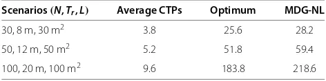
each CTP and pull data from the respective SPPs. Table 2 illustrates the performance comparison between MDG-NL and the optimum solution. From Table 2, we can see that MDG-NL achieved near-optimal results, especially in the first scenario. This is because a few number of CTPs are created and the best route needs no more iterations to discover. Obviously, when a network size increases, the optimal solution needs more iterations to discover the optimal path which costs more time (i.e. exponential time) to finish the job. Contradictory to the optimal solution, the heuristic algorithm produced a near-optimal solution within a reasonable time.

6.3 Performance of MDG-NL vs. SPT-DGA

In this sub-section, we present the simulation results and compare them with the polling-based approach (i.e. SPT-DGA) [1]. For more clarification on the difference between the polling-based approach and the turning-based approach, a comparison between SPT-DGA and MDG-NL is presented in Table 3.

In this simulation, a general sensor network with N sensor nodes is uniformly random distributed over the deployment field(Lmetre×Lmetre)with the transmission

rangeTrmetrefor each sensor considered. In addition, the

BS is located at the centre of the deployment field. The local data is aggregated to the respective SPPs within relay hop bounddas illustrated in Algorithm 1.

Three performance metrics considered in this simula-tion are the tour length of ME, the latency to deliver the data to the BS and the total energy consumed during the data gathering process. We adopt theNN algorithm [37] for the purpose of moving through CTPs in order to gather data from SPPs. ThisNNalgorithm allows the ME to start from the BS and visit the nearest CTP and then find the nearest CTP to the previous one eventually until it returns to the BS.

Due to the randomness of the network topology, the individual performance point in the figures is the average result obtained based on 500 simulations. The variation in the simulation results is presented using Equation 8 [38] with a confidence interval of 95%.μ,σandnrepresents the mean value, standard deviation and number of simula-tions obtained, respectively. The performance gain is cal-culated to show the variation results between MDG-NL and SPT-DGA based on Equation 9. x represents the results produced using MDG-NL, and x represents the

Table 2 Comparison with the optimal solution

Scenarios₍_N,_T_r,_L₎ Average CTPs Optimum MDG-NL

30, 8 m, 30 m2 _3.8 _25.6 _28.2

50, 12 m, 50 m2 _5.2 _51.8 _59.4

100, 20 m, 100 m2 _9.6 _183.8 _218.6

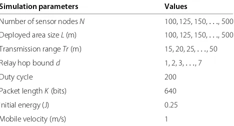
results produced using SPT-DGA. We used a first-order radio model as in [39] in order to compute the power con-sumption at each sensor node as depicted in Equations 1 and 11. In a duty cycle, each sensor node generates a fixed size packet and sends it to its parent. The in-network aggregation used here has size reduction by merging the data packets received from all children of the current node and produces one data packet to the upper level. The sim-ulation parameters used in this simsim-ulation are presented in Table 4.

Estimate margin of error=μ±1.96

_σ

√

n

(8)

Performance gain=

Figure 6a illustrates the performance of SPT-DGA and MDG-NL as a function of bounded relay hopdin terms of tour length. The extreme case when d is set to zero means no relay available and the ME should visit each sen-sor node to pull its data. To illustrate the effect of hop count on the data gathering tour path,N,LandTrare set to be constant and assigned the values 200, 200 m and 30 m, respectively. It can be seen that when the hop count (d) increases, the tour length needed for the ME to traverse a deployment field is shortened in both algorithms. This is due to the increasing hierarchical level of each geomet-ric tree rooted to each SPP with more affiliated sensors forwarding their data to the same SPP. In addition, these SPPs are closer to each other and are also located closer to the BS. Minimizing the number of CTPs visited by the ME causes the tour length to be minimized in comparison with the SPT-DGA algorithm. Furthermore, in all cases, MDG-NL outperforms SPT-DGA with almost 12.5%. The variance in tour length increases whendis decreased, and this is because more SPPs are created causing a longer tour length as the ME should visit each one separately in the SPT-DGA algorithm.

(13)

Table 3 Comparison between SPT-DGA and MDG-NL

Feature/approach Polling-based approach (SPT-DGA) Turning-based approach (MDG-NL)

Motion pattern Controllable Controllable

Pausing location Mobile collector pauses at each PP Mobile collector pauses at each CTP

Moving trajectory Starts from the BS and visits each PP before eventually returning to the BS

Starts from the BS and visits each CTP before eventually returning to the BS

Local data aggregation Bounded multi-hop relay Bounded multi-hop relay

Data uploading With each pause location, the ME pulls the data from a single PP

With each pause location, the ME pulls the data from two SPPs

The BS Located at the centre of the deployment field Located at the centre of the deployment field

SPT Builds to the nearest node to the BS Builds to the BS

Latency Depends on the velocity of ME and the locations of each PP

Depends on the velocity of ME and the locations of each CTP

Power consumption Depends on the bounded relay hop, node distribu-tion and transmission range

Depends on the bounded relay hop, node distribution and transmission range

algorithm with almost 11.3% and 8.8% whendis set to 2 and 3, respectively.

Figure 6c illustrates the performance of SPT-DGA and MDG-NL as a function of the number of nodesN.L,Tr anddare set to 200 m, 30 m and 2, respectively. It can be noticed that when the sensor nodeNincreases, the tour length in both algorithms increases too. The impact of increasingNon the tour path is obvious at the beginning (i.e.Nis below 300), but with continued increase to a suffi-ciently large number, the impact on the tour length will be less compared with the beginning and the total numbers of SPPs and CTPs are most likely stable. This is because the sensors are more densely scattered and more sensors are affiliated with the same SPP. The performance gain of MDG-NL over SPT-DGA in all cases is almost 10.7%.

Figure 6d illustrates the performance of SPT-DGA and MDG-NL as a function of deployed fieldL.Tr,Nanddare set to 30 m, 400 and (2,3), respectively. It can be noticed that whenL increases, the tour length also increases in both algorithms. This is because sensors become more sparsely distributed and less sensors are affiliated with the same SPP (i.e. the number of SPPs increases). In

Table 4 Simulation parameters

Simulation parameters Values

Number of sensor nodesN 100, 125, 150,. . ., 500

Deployed area sizeL(m) 100, 125, 150,. . ., 500

Transmission rangeTr(m) 15, 20, 25,. . ., 50

Relay hop boundd 1, 2, 3,_{. . .}, 7

Duty cycle 200

Packet lengthK(bits) 640

Initial energy (J) 0.25

Mobile velocity (m/s) 1

addition, the proposed algorithm outperforms SPT-DGA in all cases due to extraction of the gathered data from two SPPs within one pause of ME. The average percentage of MDG-NL enhancement over SPT-DGA in all cases is almost 10.36% and 11.03% when hop countdequals 2 and 3, respectively.

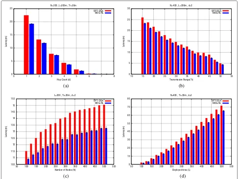
Figure 7a illustrates the performance of SPT-DGA and MDG-NL as a function of bounded relay hopdin terms of data gathering latency. The latency of ME is propor-tional to the tour length needed to collect the data from respective nodes and the velocity of ME. The number of nodes selected as SPPs and CTPs and their locations are two factors affecting the data gathering latency. These nodes become less and are located near the BS when the hop count (d) is increased, and this leads to lower latency which shortens the time needed for the ME to visit all respective nodes before eventually returning to the BS. This is done because a few number of SPPs and CTPs are created. In all cases, MDG-NL outperforms SPT-DGA in terms of data gathering latency. For the case whend is equal to 7, the BS becomes the root of the shortest path tree in both algorithms and the data traverses via multi-hop only, omitting the need for the ME.

(14)

0

Figure 6SPT-DGA vs. MDG-NL in terms of tour length (m).(a)Hop count.(b)Transmission range.(c)Number of nodes.(d)Deployed area size.

certain level makes a BS neighbor to each sensor node. Thus, the data is sent directly to the BS via single hop which leads to minimizing the latency to the lowest level.

Figure 7c illustrates the performance of SPT-DGA and MDG-NL as a function of the number of nodesNin terms of data gathering latency. It is obvious that when the num-ber of nodesNis smaller, a few SPPs and CTPs are created and the ME will need no much time to gather the data from all the respective nodes. On the other hand, whenN increases, the SPPs and CTPs increase and the ME needs more time to deliver the data to the BS. By increasing the number of nodes (i.e. a dense network), the over-lapping SPPs increase too. Thus, in all cases, MDG-NL outperforms SPT-DGA in terms of data gathering latency. Figure 7d illustrates the performance of SPT-DGA and MDG-NL as a function of deployed field L in terms of data gathering latency. Increasing the deployed area size leads to increasing the latency of data gathering, and this

is due to sparse SPPs. However, the existence of over-lapped SPPs gave the MDG-NL algorithm an advantage over the SPT-DGA algorithm by minimizing the tour length of ME required to visit each CTP to pull the data from all SPPs. Thus, the MDG-NL algorithm outperforms the SPT-DGA algorithm in data gathering latency in all cases.

(15)

0 5 10 15 20 25

0 1 2 3 4 5 6 7 8

Latency(m)

Hop Count (d) N=200 , L=200m , Tr=30m

SPT-DGA MDG-NL

(a)

0 5 10 15 20 25 30

10 15 20 25 30 35 40 45 50 55

Latency(m)

Transmission Range(Tr) N=400 , L=200m , d=2

SPT-DGA MDG-NL

(b)

10.5 11 11.5 12 12.5 13 13.5 14 14.5 15 15.5

50 100 150 200 250 300 350 400 450 500 550

Latency(m)

Number of Nodes (N) L=200 , Tr=30m , d=2

SPT-DGA MDG-NL

(c)

0 10 20 30 40 50 60 70 80

50 100 150 200 250 300 350 400 450 500 550

Latency(m)

Deployed Area (L) N=400 , Tr=30m , d=2

SPT-DGA MDG-NL

(d)

Figure 7SPT-DGA vs. MDG-NL in terms of data gathering latency (min).(a)Hop count.(b)Transmission range.(c)Number of nodes. (d)Deployed area size.

Second, the shortest path tree builds to the BS in MDG-NL unlike in SPT-DGA in which it builds to the nearest node to the BS. Overall, maintaining the energy consump-tion at a certain level while minimizing the tour length of ME is a challenge due to the trade-off between energy consumption and tour length in mobile data gathering [1]. Figure 8b illustrates the performance of SPT-DGA and MDG-NL as a function of transmission rangeTrin terms of total energy consumed. It is obvious that when the transmission range Tr has the smallest value, the total energy consumed is minimized, and this is due to two reasons. First, the power consumption due to the com-munication is affected directly by the distance (i.e. a short distance needs less energy and vice versa). Second, mul-tiple disconnected networks are created which leads to increasing the number of SPPs and CTPs with a few sen-sors affiliated. In other words, the level of each geometric tree is limited and sometimes there is only one level. Fur-thermore, increasing the transmission range forces the

sensors to send their data to the farthest neighbor towards the BS. Thus, the hierarchy level of the shortest tree is decreased with creating a few polling nodes (i.e. SPPs and CTPs). In both algorithms, the total energy consumed is almost similar to each other.

(16)

3.5

Figure 8SPT-DGA vs. MDG-NL in terms of total energy consumption (J).(a)Hop count.(b)Transmission range.(c)Number of nodes. (d)Deployed area size.

both algorithms, the total energy consumed is closer to each other.

Figure 8d illustrates the performance of SPT-DGA and MDG-NL as a function of deployed field L in terms of total energy consumed. It is noticed that when deployed area Lhas the smallest value (i.e. 100), the power con-sumption is mostly the highest in comparison to other values. This is because the sensor network is fully con-nected and all communications required to send the data are computed. On the other hand, whenLhas the highest value (i.e. 500), the power consumption is minimized. This is because multiple disconnected networks are created with a few sensors. Thus, the communications required to deliver the data to the nearest SPP are minimized. In addi-tion, some sensors are located far from any other network. However, MDG-NL maintains the power consumption within a certain level, and the power consumptions for both algorithms are similar.

7 Conclusions and future work

(17)

the developed algorithms and to study the impact on the performance measures in comparison to the SPT-DGA algorithm. MDG-NL has proven to successfully modu-late and significantly improve the tour length of ME and the latency of data gathering. However, due to the trade-off between power consumption and tour length of ME, MDG-NL maintains the power consumption to be within an acceptable level in comparison to the SPT-DGA algo-rithm. The enhancement of applying multiple MEs with region division is an interesting area in the future. With this enhancement, each ME is appointed to a predefined sub-region, which is a part of the deployment field.

Competing interests

The authors declare that they have no competing interests.

Received: 15 July 2013 Accepted: 6 March 2014 Published: 31 March 2014

References

1. M Zhao, Y Yang, Bounded relay hop mobile data gathering in wireless sensor networks. IEEE Trans. Comput.61(2), 265–277 (2012) 2. Y Bi, N Li, L Sun, DAR: an energy-balanced data-gathering scheme for

wireless sensor networks. Comput. Commun.30(14–15), 2812–2825 (2007). http://www.sciencedirect.com/science/article/pii/ S0140366407002150. [Network Coverage and Routing Schemes for Wireless Sensor Networks]

3. A Tarachand, V Kumar, A Raj, A Kumar, P Jana, An energy efficient load balancing algorithm for cluster-based wireless sensor networks, inAnnual IEEE India Conference (INDICON ‘12)(Kochi, 2012), pp. 1250–1254 4. S Bandyopadhyay, Q Tian, E Coyle, Spatio-temporal sampling rates and

energy efficiency in wireless sensor networks. IEEE/ACM Trans. Netw. 13(6), 1339–1352 (2005)

5. M Takruri, S Rajasegarar, S Challa, C Leckie, M Palaniswami,

Spatio-temporal modelling-based drift-aware wireless sensor networks. IET Wireless Sensor Syst.1(2), 110–122 (2011)

6. U Jang, S Lee, S Yoo, Optimal wake-up scheduling of data gathering trees for wireless sensor networks. J. Parallel Distributed Comput.72(4), 536–546 (2012). http://www.sciencedirect.com/science/article/pii/ S0743731512000196

7. R Bista, YK Kim, YH Choi, JW Chang, A new energy-balanced data aggregation scheme in wireless sensor networks, inInternational Conference on Computational Science and Engineering, CSE ‘09,vol. 2 (Vancouver, 29–31 Aug 2009), pp. 558–563

8. T Liu, F Li, Power-efficient clustering routing protocol based on applications in wireless sensor network, in5th International Conference on Wireless Communications, Networking and Mobile Computing, WiCom ‘09 (Beijing, 24–26 Sept 2009), pp. 1–6

9. F Ren, J Zhang, T He, C Lin, S Ren, EBRP: energy-balanced routing protocol for data gathering in wireless sensor networks. IEEE Trans. Parallel Distributed Syst.22(12), 2108–2125 (2011)

10. Z Ding, N Yamauchi, An improvement of energy efficient multi-hop time synchronization algorithm in wireless sensor network, in2010 IEEE International Conference on Wireless Communications, Networking and Information Security (WCNIS ‘10)(Beijing, 2010), pp. 116 –120 11. Jh Zhang, H Peng, Y Tian tian, Tree-adapting: an adaptive data

aggregation method for wireless sensor networks, in2010 6th International Conference on Wireless Communications Networking and Mobile Computing (WiCOM ‘10)(Chengdu, 2010), pp. 1–5

12. TT Nguyen, VD Nguyen, Optimizing the operating time of wireless sensor network. EURASIP J. Wireless Commun. Netw.2012, 1–12 (2012) 13. RC Shah, S Roy, S Jain, W Brunette, Data mules: modeling and analysis of a

three-tier architecture for sparse sensor networks. Ad Hoc Networks.1(2), 215–233 (2003)

14. M Zhao, M Ma, Y Yang, Efficient data gathering with mobile collectors and space-division multiple access technique in wireless sensor networks. IEEE Trans. Comput.60(3), 400–417 (2011)

15. C Wang, H Ma, Data collection in wireless sensor networks by utilizing multiple mobile nodes, inSeventh International Conference on Mobile Ad-hoc and Sensor Networks (MSN ‘11)(Beijing, 16–18 Dec 2011), pp. 83–90 16. M Ma, Y Yang, M Zhao, Tour planning for mobile data-gathering

mechanisms in wireless sensor networks. IEEE Trans. Vehicular Technol. 62(4), 1472–1483 (2013)

17. K Almi’ani, A Viglas, L Libman, Mobile element path planning for time-constrained data gathering in wireless sensor networks, in24th IEEE International Conference on Advanced Information Networking and Applications (AINA ‘10)(Perth, 20-23 Apr 2010), pp. 843–850

18. A Kumar, K Sivalingam, Energy-efficient mobile data collection in wireless sensor networks with delay reduction using wireless communication, in Second International Conference on Communication Systems and Networks (COMSNETS ‘10)(Bangalore, 5–9 Jan 2010), pp. 1–10

19. D Jea, A Somasundara, M Srivastava, Multiple controlled mobile elements (data mules) for data collection in sensor networks, inProceedings of the First IEEE International Conference on Distributed Computing in Sensor Systems, DCOSS ‘05(Springer Berlin, 2005), pp. 244–257. http://dx.doi.org/ 10.1007/11502593_20.

20. G Xing, M Li, T Wang, W Jia, J Huang, Efficient rendezvous algorithms for mobility-enabled wireless sensor networks. IEEE Trans. Mobile Comput. 11, 47–60 (2012)

21. M Ma, Y Yang, SenCar: an energy-efficient data gathering mechanism for large-scale multihop sensor networks. IEEE Trans. Parallel Distributed Syst. 18(10) (1476)

22. RW Pazzi, A Boukerche, Mobile data collector strategy for delay-sensitive applications over wireless sensor networks. Comput. Commun.31(5), 1028–1039 (2008). http://www.sciencedirect.com/science/article/pii/ S0140366407005464. [Mobility Management and Wireless Access] 23. FJ Wu, CF Huang, YC Tseng, Data gathering by mobile mules in a spatially

separated wireless sensor network, inProceedings of the 2009 Tenth International Conference on Mobile Data Management: Systems, Services and Middleware, MDM ‘09(IEEE Washington, DC, 2009), pp. 293–298. http://dx.doi.org/10.1109/MDM.2009.43.

24. M Marta, M Cardei, Improved sensor network lifetime with multiple mobile sinks. Pervasive and Mobile Comput.5(5), 542–555 (2009). http:// www.sciencedirect.com/science/article/pii/S1574119209000029 25. S Vupputuri, KK Rachuri, CSR Murthy, Using mobile data collectors to

improve network lifetime of wireless sensor networks with reliability constraints. J. Parallel Distributed Comput.70(7), 767–778 (2010). http:// www.sciencedirect.com/science/article/pii/S0743731510000456. 26. JP Sheu, PK Sahoo, CH Su, WK Hu, Efficient path planning and data

gathering protocols for the wireless sensor network. Comput. Commun. 33(3), 398–408 (2010). http://www.sciencedirect.com/science/article/pii/ S014036640900276X.

27. H Nakayama, Z Fadlullah, N Ansari, N Kato, A novel scheme for WSAN sink mobility based on clustering and set packing techniques. IEEE Trans. Automatic Control.56(10), 2381–2389 (2011)

28. K Lin, M Chen, S Zeadally, JJPC Rodrigues, Balancing energy consumption with mobile agents in wireless sensor networks. Future Gener. Comput. Syst.28(2), 446–456 (2012). http://dx.doi.org/10.1016/j.future.2011.03.001. 29. K Dantu, M Rahimi, H Shah, S Babel, A Dhariwal, G Sukhatme, Robomote:

enabling mobility in sensor networks, inIPSN ’05: Proceedings of the 4th International Symposium on Information Processing in Sensor Networks (Los Angeles, 2005), pp. 404–409

30. G Xing, T Wang, W Jia, M Li, Rendezvous design algorithms for wireless sensor networks with a mobile base station, inProceedings of the 9th ACM International Symposium on Mobile Ad Hoc Networking and Computing (Hong Kong, 26–30 May 2008), pp. 231–240

31. O Chipara, Z He, G Xing, Q Chen, X Wang, C Lu, J Stankovic, T Abdelzaher, Real-time power-aware routing in sensor networks, in14th IEEE International Workshop on Quality of Service, IWQoS ‘06(New Haven, 2006), pp. 83–92

32. M Johnson, M Healy, P van de Ven, M Hayes, J Nelson, T Newe, E Lewis, A comparative review of wireless sensor network mote technologies, inIEEE Sensors ‘09(Christchurch, 2009), pp. 1439–1442

33. CPLEX package. http://www.ilog.com/products/cplex/. Accessed 12 Nov 2012

34. AMPL package. http://www.ampl.com/. Accessed 12 Nov 2012 35. M Zhao, Design and optimization on mobile data gathering in wireless

(18)

36. B Gavish, Formulations and algorithms for the capacitated minimal directed tree problem. J. ACM.30, 118–132 (1983). http://doi.acm.org/10. 1145/322358.322367.

37. T Cormen, C Leiserson, R Rivest, C Stein,Introduction to Algorithms (MIT Press, Cambridge, 2001)

38. AR Rudnicka, Essential medical statistics (2nd edn). Betty R. Kirkwood and Jonathan A. C. Sterne, Blackwell Science, Oxford, 2003. No. of pages: 512. Price: £22.95. ISBN 0-86542-871-9. Stat. Med.24(5), 824–824 (2005) 39. W Heinzelman, A Chandrakasan, H Balakrishnan, Energy-efficient

communication protocol for wireless microsensor networks, in Proceedings of the 33rd Annual Hawaii International Conference on System Sciences,vol. 2 (Maui, 2000), p. 10

doi:10.1186/1687-1499-2014-51

Cite this article as: Ghalebet al.: Predetermined path of mobile data gathering in wireless sensor networks based on network layout.EURASIP Journal on Wireless Communications and Networking20142014:51.