A novel local and nonlocal total variation combination method for image restoration in wireless sensor networks

R E S E A R C H

Open Access

A novel local and nonlocal total variation

combination method for image restoration

in wireless sensor networks

Mingzhu Shi

and Liang Feng

Abstract

In this paper, we propose a novel local and nonlocal total variation combination method for image restoration in wireless sensor networks (WSN), which plays an important role in improving the quality of the transmitted image. First, the degrade image is preprocessed by an image smoothing scheme to divide the image into two regions. One contains edges and flat regions by the local TV term. The other is rich in image details and regularized by the nonlocal TV term. Then, the alternating direction method of multipliers (ADMM) algorithm is adopted to optimize the complex object function, and two key parameters are discussed for better performance. Finally, we compare our method with several recent state-of-the-art methods and illustrate the efficiency and performance of the proposed model by experimental results in peak signal to noise ratio (PSNR) and computing time.

Keywords:Image restoration, Nonlocal total variation, Alternating direction minimization of multiplier, Overlapping group sparsity

1 Introduction

With the rapid development of wireless sensor networks, there are higher requirements for signal transmission

and processing [1–4]. However, for such a

two-dimensional image signal, it is inevitably degraded in the process of image acquisition, transmission and process-ing, and image restoration techniques are needed to im-prove the quality of the obtained image. Image restoration is one of the most fundamental issues in im-aging science and other important applications. It plays an important role in many mid-level and high-level image processing tasks. In this paper, we focus on spatially invariant system and formulate a common deg-radation model as

g¼hf þn; ð1Þ

where g is the blurred and noisy image,f is the desired true image, * represents the convolution, and n denotes

the additive Gaussian white noise with zero mean. h is the linear spatially invariant blur kernel, which is usually modeled as a blurring matrix constructed from the discrete point spread function (PSF). If the PSF is known, the problem is non-blind deconvolution. If the PSF is unknown, then the given problem becomes blind deconvolution. In this paper, we only focus on the non-blind image restoration.

1.1 Problem setup

For the image restoration problem, we seek to

esti-mate the original image f by the following variational

formulation:

arg min

f

1

2kg−hfk 2

2þλϕð Þf

: ð2Þ

where ‖.‖2 denotes the Euclidean norm, ϕ(f) is usually

called the regularization term, and λ> 0 is a regularization parameter that controls the balance be-tween the above fidelity term and regularization term. Even if the blur kernel is known, the problem is still highly ill-posed and there is difficulty in recovering the original sharp image. This is because that the blur kernel is a kind of a low-pass filter, which tends to reduce the * Correspondence:[email protected]

1

Tianjin Key Laboratory of Wireless Mobile Communications and Power Transmission, Tianjin Normal University, Tianjin 300387, China 2_{College of Electronic and Communication Engineering, Tianjin Normal} University, Tianjin 300387, China

Full list of author information is available at the end of the article

high-frequency information such as textures and edges. Hence, it needs to be regularized by a proper constraint model. The classical regularization model is the TV model, which is referred to the local TV [5] with the form

image and is often defined as

f sent the local first-order differences offin the horizon-tal and vertical directions respectively. The local TV model has been proven to have good performance in preserving edges due to its linear penalty on differences between adjacent pixels. However, it yields to staircase artifacts that smooth image details. Therefore, it is of great importance to model the appropriate prior know-ledge from nature images or impose more appropriate prior assumption to constrain the solution. Actually, the underlying motivation in this paper is to establish appropriate regularization terms and improve the effi-ciency of the numerical algorithm for the complex ob-ject function.

1.2 Related works

In recent years, the nonlocal TV has been successfully used in image processing tasks [6, 7]. It uses the whole image pixel information not the adjacent pixel informa-tion and combines the variainforma-tional framework and the nonlocal self-similarity constraint to restore the image details. This is the main difference with the local TV model. However, if the nonlocal self-similarity constraint is considered as the only constraint, similar image struc-tures still cannot be estimated accurately. When the TV model and the nonlocal self-similarity constraint are both used on the entire image, the performance of their method will be compromised under the limitation of the TV model [8]. Besides, since the nonlocal total variation requires weighted difference between pixels in the whole image, it is more time consuming and needs more effi-cient algorithms. The Spliting-Bregman method has been proposed to solve the nonlocal TV image restor-ation problem, but the efficiency is unsatisfactory [9, 10]. It not only needs the outer iteration in the subproblem but also the inner iterations for the nonlocal Laplacian operator. Zhu et al. propose an efficient primal-dual hy-brid gradient algorithm, which alternates between the

primal and dual formulations for total variation [11]. A unified primal-dual algorithm framework is proposed to resolve the local total variation problem with L1 basis pursuit and TV-L2minimization [12]. Bonettini et al. es-tablish the convergence of a general primal-dual method for nonsmooth convex optimization problems, whose structure is typical in the imaging framework [13]. In these approaches, many parameters have to be chosen and causes time consuming. To overcome this draw-back, an alternating direction minimization method of multipliers (ADMM) has been widely used in recent image-processing tasks [14, 15]. Its outstanding per-formance is that there is no need to resolve the sub-problems and no inner iterations. Hence, the problem needs to be solved from two aspects: one is how to choose a good regularization functional φ(f), which is an active research area in image science, and the other is how to shorten the computation time without yielding staircase artifacts, which is also a challenging problem.

The rest of the paper is organized as follows. In Section 2, we introduce the definition of the nonlocal total variation and the principle of the overlapping group sparsity and the ADMM algorithm. They are the essential tools in our method. Section 3 intro-duces the object function of the proposed model and discusses the parameter selection criteria. In Section 4, we carry out experiments and compare ours with other state-of-the-art methods. Finally, we make a conclusion in Section 5.

2 Preliminaries

2.1 Nonlocal total variation

Firstly, we give the following notations that will be used in this paper. Assuming the size of images in this paper

is m ×n, and the image matrix rows from stacking up

are denoted as mn vectors. Denote the Euclidean space

RmnasVand define Q=V×V. Theith components of

x∈V and y∈Q are denoted as xi∈R and y_i¼

y_ið Þ1_;y ið Þ2

ð ÞT_∈

R2, respectively. Inner products and Euclidean norms are defined as

x;x the vertical and horizontal directions, and we have

Dfi= [(D(1)fi), (D(2)fi)]T for each f∈V. By staking the

ith rows of D(1) and D(2) together, we get a tow-row

finite difference operator as D= [(D(1))T, (D(2))T]T∈

R2mn×mn. We consider Df∈Q and assume images in

this paper under the periodic boundary condition. The discrete gradient operators are defined by

Dð Þ1f

Then, we use the definitions and notations of the local total variation introduced in [16]. LetΩ⊂R2and x∈Ω, fined based on the image u. The graph divergence div_ω of a vectorp:Ω×Ω→Rcan be defined as The weight function is defined as the nonlocal means weight function:

where Ga is the Gaussian kernel with standard deviation

a,his the filtering parameter related to the standard vari-ance of the noise, and the ⋅ in f(x+⋅) denotes a square patch centered by pointx.When the reference imagefis known, the nonlocal means filter is a linear operator. Now, we can define the nonlocal TV norm with the iso-tropicL1norm of the weight graph gradient∇ωu(x):

The main purpose of the nonlocal regularization is to generalize the local gradient and divergence concepts into the local form. Generally, a reference image is expected as close as possible to the original image to obtain the weights more exactly. However, it is hard to get the price weights between the pixels because the original image is degraded in the image formation process. Thus, the weights have to be calculated according to a preprocessed image. In this paper, the degraded image is preprocessed by an image smoothing scheme, which is mentioned to optimize theL0norm of the image gradient.

2.2 Overlapping sparsity prior

The sparsity-based regularization has obtained promi-sing results for various ill-posed image restoration problems. Group sparsity concept was first used in the one-dimension denoising problem [17, 18]. Con-sidering that groups of large values may arise any-where in the signal domain, a group of large values may straddle two of the predefined groups, especially in general signal denoising and restoration problem. Hence, if the group structure is treated as a prior, it is suitable to formulate the problem into overlapping groups. And it is natural to extend the overlapping group sparsity prior to solve the two-dimension prob-lem such as image restoration. It has been used as a penalty term for TV models and proven to be effect-ive for alleviating staircase effect [15].

In [15], the vectors∈Rnwith ak-point group has been defined as

si;k¼½s ið Þ;⋯;s ið þk−1Þ∈Rk ð10Þ

Here,si,kdenotes a block ofkcontiguous samples ofs

starting from the ith index. A group sparsity regularizer is defined as

ζð Þ ¼s X

n i¼1

si;k ₂ ð11Þ

For the two-dimensional case, a k×k point group of

the imagef∈Rn×nis defined as ping group sparsity (OGS) functional of a two-dimensional array can be defined as

φOGSð Þ ¼f

The regularization term ϕ(f) based on the image

gradient in the vertical and horizontal direction is de-noted as

It is a special case that is commonly mentioned as

ani-sotroapic TV functional if k= 1, and the usual TV

ΦTVð Þ ¼f

where the discrete gradient operator∇:Rmn_→

R2 ×mnis defined by (∇f)i,j= ((D(1)f)i,j, (D(2)f)i,j).

2.3 ADMM

ADMM is a special splitting case of the augmented Lagrangian method by splitting the complex problem into simpler subproblems, which can be easily solved by efficient operators, such as DFT and shrinkage op-erator. It also can take advantage of separable struc-tures of the split object functions, which allow a straightforward treatment of various regularize terms,

such as total variation regularization [19]. The

ADMM algorithm resolves a linear system like a matrix transformation that makes the problem two-sided. On the one hand, the transformed matrix is re-lated to the Hessian transform of the objective func-tion carrying the second-order informafunc-tion. This fact meets the excellent performance of computational ef-ficiency, which has been proven to be faster than the classical iterative shrinkage thresholding (IST) algo-rithms [20], even than their improved versions [21]. On the other hand, due to the typical huge size of the inversion, it is limited to resolve the problem that can be handled efficiently using some particular structure. In this paper, we use the fast Fourier

transform (FFT) to improve the efficiency of

ADMM. The convergence is guaranteed by the clas-sical ADMM theory in literatures [22, 23]. In this subsection, we briefly review its basic theory for an intuitive understanding.

The ADMM theory was proposed to solve the optimization problem with the following constrained separable subproblem

miny₁ð Þ þx1 y2ð Þ;x2 s:t:A1x1þA2x2¼a ð16Þ

where xi∈Xi, i= 1, 2, yi:Xi→R are closed convex

function, Xi∈Rmi are nonempty closed convex sets, Ai

∈Rlmi _{are linear transforms, and a}∈_Rl _{is a given} vec-tor. With q∈Rl as a Lagrange multiplier to the linear constraint, the augmented Lagrangian function for the problem (16) is

Here, δis the penalty parameter that controls the lin-ear constraint. According to the theory of the ADMM, optimal solutions is equivalent to finding a saddle point

L x ₁;x₂;q by the alternative minimizing scheme, such

as keeping x2 and q fixed when minimizing L with

re-spect tox1. Then, we obtain the following ADMM itera-tive minimizing algorithm:

Iterative strategy of two subproblems is in the Gauss-Seidel fashion and thus the variables x1 and x2 can be solved separately in the alternating order. In [24], Eckstein and Bertsekas demonstrated that ADMM could be interpreted as an application of the proximal point al-gorithm. Meanwhile, a convergence result was proved for ADMM that allowed approximate computation of

xk₁þ1 and xk₂þ1. Here, we restate their result as it applies to (14) under slightly weaker assumptions and in the case without over or under relaxation factors.

Theorem 2.1 (Eckstein, Bertsekas [24]) Consider the problem (13) where y1and y2are closed proper convex

3 Proposed model and numerical algorithm

3.1 Image region division

The image is preprocessed by an image smoothing

scheme same as [25], take experiments on “Babara”

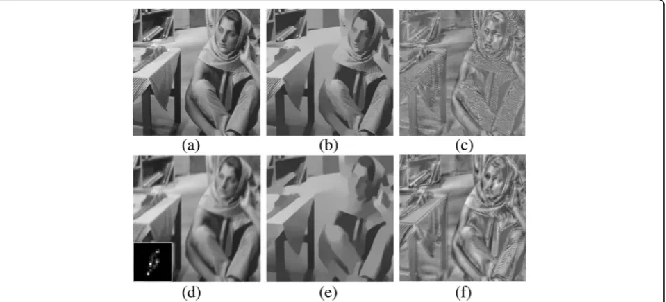
as an example. As shown in Fig. 1, Fig. 1a is the ori-ginal image, Fig. 1b is the salient edges and constant regions of (a), and Fig. 1c is the details of (a) and ob-tained by (a) minus (b). Fig. 1d is the blurred image and the blur kernel is shown in the lower left, with the size 19 × 19. Figure 1e and (f ) are edges and constant regions, and details of (d), respectively. Comparing the extracted edges and constant regions in Fig. 1b, e, we cannot see much obvious difference, although the blurred image (d) is seriously damaged. Meanwhile, the details of the blurred image shown in (f ) are more clear than those of the original image (a), from the point of view.

3.2 Novel nonlocal total variation

To overcome the drawback of the local TV model, researchers have proposed to combine the nonlocal TV and the TV model to resolve some image pro-cessing tasks. Tang et al. [26] combined a local TV filter and the nonlocal means algorithm for image denoising. In his work, a local TV filter was used only for the rare patches, such as special edges and rare detail patches, and the nonlocal means algorithm was used for the rest. However, the model is limited to image deblurring because the image structures have been severely damaged and the similar structures cannot be found accurately. Inspired, we apply the nonlocal TV regularization only for the image details

to protect the detail information and the overlapping group sparsity prior for the sparser image representa-tion constraint. Especially in our previous work [27], it has been proven the performance of using the over-lapping group sparsity prior in suppressing the stair-case effect.

Now, a novel nonlocal TV based image restoration model is defined as follows:

min

f S;f D

( λ

2khfSþhfD−gk

2

2þα ϕ Dð Þ1fS

þϕ Dð Þ2fS

þk∇ωfDk )

;

ð18Þ

where λ and α are regularization parameters. The ori-ginal image fis divided as fS and fD by the above

men-tioned gradient extraction scheme.fS denotes the salient

edges and constant regions, and fD denotes the image

details. In order to apply the ADMM idea, we introduce auxiliary variables v1=D(1)f, v2=D(2)f, and z=f.

Com-pared with the standard ADMM algorithm in Eq. (16), the problem (18) satisfies the proposed framework with the following specification:

(1)x1≔f;x2≔½v1;v2;z;

(2)y₁ð Þ ¼x1 λ₂khfSþhfD−gk

2 2,y2(x2)

=α‖ϕ(D(1)f_S) +ϕ(D(2)f_S)‖+‖∇_ωf_D‖.

Then, the Augmented Lagrangian function of the minimization problem (18) is defined as follows:

LAðf;v;z;ε;ηÞ ¼

where β1,β2> 0 are linear constraints corresponding to the auxiliary variables z and v, and ε and η are the Lagrange multipliers. Starting at f=fk, ε=εk, and η=ηk, applying ADMM yields the iterative scheme

vkþ1

As the theoretical analysis in [22], positive values of the parametersβ1,β2, andγcan ensure the convergence of ADMM, and we will be set them to specified values in the later experiments.

3.3 Numerical algorithm

According to the ADMM in Algorithm 1, we employ the alternative optimization to estimate the divided image regionsfSandfD.

The minimization of Eq.(23) with respect to fS is a

least square problem and can be resolved by the fast

Fourier transform (FFT), which only requiresO(nlog(n)) arithmetic operations, here n represents the size of the given image. The corresponding normal equation of Eq.(23) is

where H denotes the blurring matrix formed by h. Considering v1 and v2 with the same expression, the

subproblem corresponds to the following optimization problem

which can be attacked with the extremely fast shrinkage formula and obtain

4 Results and discussion

4.1 Experimental settings

In order to demonstrate the viability and efficiency of the proposed method, experiments are carried out on various image and kernels and compared with other state-of-the-art methods. Test images are some

clas-sical images, such as “Boat” with the size 128 × 128,

“Cameraman” with the size 256 × 256, “Lena” with

the size 512 × 512, “Babara” with the size 512 × 512,

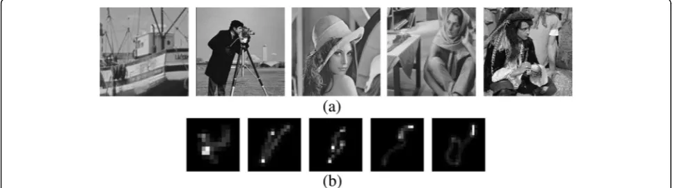
and “Man” with the size 1024 × 1024. And five different motion blur kernels are used in the experiments. They are freely available from http://www.wisdom.weizmann. ac.il/~levina/ and frequently used in present researches for image restoration, as shown in Fig. 2a. The size of each kernel is 13 × 13, 17 × 17, 19 × 19, 21 × 21, and 23 × 23, as shown in Fig. 2b. We also try the average blur kernel and add the Gaussian noise to degrade the image. The stop cri-terion is ‖fm+ 1−fm‖2/‖fm‖2< 0.001. The PSNR is used to evaluate the quality of recovery results. All experiments are conducted by Matlab programming on a desktop PC with 2.3GHz Interl Core computer and 4.0 GB memory.

4.2 Parameters setting The PSNR is defined as

PSNR¼10 lg 255

2_MN

PM i¼1

PN j¼1

^

f ið Þ;j−f ið Þ;j

h i2; ð28Þ

where ^f ið Þ;j denotes the recovered image and f(i,j) de-notes the true image. As mentioned, the fast Fourier transforms in the algorithm, boundary problems needs to be processed; otherwise, it will affect the PSNR ser-iously. The “edgetaper” function in Matlab is chosen as the periodic boundary condition. There are many auxil-iary variables and coefficients in the object formulation that the form seems very complicated, as shown in Eq.(19) and (23), especially in the algorithm description and theoretical analysis. In actual fact, auxiliary variables

are helpful in programming and reducing computational redundancy.

Considering the penalty parametersβ1,β2, andγ, theor-etically, any positive values ensure the convergence of ADMM. In practice, there are usual two ways to deter-mine them. One tries some values and picks a certain value with satisfactory performance; the other applies self-adaptive adjustment rules with an arbitrary initial guess but requires expensive computation. In our experi-ence, a well-tuned constant value has the same perform-ance to the value obtained by the self-adaptive strategy.

For our proposed model, we tune and set β1 = 0.025

and β2 = 0.05. Parameters λ = 0.04, α = 0.05, and

γ = λ/3 = 0.012 are chosen based on the experience

of our previous work; for more details, refer to. In this subsection, we mainly focus on the iterative

par-ameter k and the window of nonlocal TV operator. As

shown in Fig. 1, two curves are the numerical analysis of the recovery for “blurred Babara” image (512 × 512) in Fig. 1d by our proposed method. Figure 3a shows that with the iterations increasing, the objective function value is getting smaller and the algorithm tends to be stable. Figure 3b shows that PSNR has not been significantly im-proved as the number of iterations increasing to 50. Hence, in the following experiments, we set the number of iterationsk= 50.

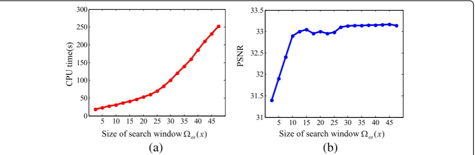
Then, the blurred image in Fig. 1d is still used to dis-cuss the weight update for nonlocal operator. An appro-priate size of the search window can guarantee the better PSNR and less CPU time. The window size is ini-tially set to 5 × 5 and increases by two steps. We also add the date with the window size 3 × 3. Computation time and PSNR are recorded at the same time, and the results are shown in Fig. 4. Figure 4a shows that as the size becomes larger, the computing time will be longer. However, PSNR has not been greatly improved in Fig. 4b. This conclusion is similar to ref. [8], which also dis-cusses the size of the search window. Particularly, al-though there are obvious difference in PSNR values when the size of search window is set to 9 × 9 and

11 × 11, the CPU time becomes longer. In order to shorten the CPU times and obtain a reasonable PSNR, we use 7 × 7 search window for the following numerical experiments.

4.3 Comparison with other state-of-art methods

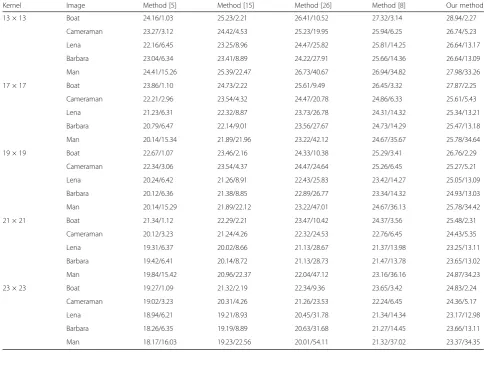
In this subsection, we use above images and blur kernels in Fig. 3 to verify the efficiency of the proposed model and compare with four state-of-the-art methods. They are the nonlocal TV method [5], the overlapping group sparsity TV method [15], the combination of local and nonlocal method using a Bregmanized operator splitting iterative scheme [26], and the nonlocal TV-based method using a linearized proximal alternating minimization algo-rithm [8]. Numerical results of the PSNR and CPU times are reported in the Table 1. It can be noted that our method obtains higher PSNR and shorter CPU times than other methods.

Because our method has the image division step in each iteration, therefore, it does not significantly shorten the computing time. As a compromise, we achieve a

better recovery effect that suppresses staircase effects and protects image details and edges. Experiments on the blurred“Babara”image in Fig. 1d are shown in Fig. 5, the avatar area in the Babara image is cropped and the details are more clear. Figure 5a is the blurred image by a 19 × 19 blur kernel. Figure 5b is the recovered image by the local TV method, which cause obvious staircase ef-fects. In Fig. 5c, the staircase effect is alleviated but unsatis-factory. In Fig. 5d, more details are restored but consumes too long time. In Fig. 5e, the method effectively saves the computing time and get a relatively satisfactory recovery effect. Our result is shown in Fig. 5f, by comparing the pat-tern on the scarf, it can be drawn that our method can sup-press staircase effects and preserve more details.

We also test on the blurred and noisy image, as shown

in Figs. 6 and 7. The image “Cameraman” with the size

256 × 256 is degraded by a 9 × 9 average kernel and Gaussian white noise withσ= 3, as shown in Fig. 6a. In Fig. 6b, there are serious staircase effects by the local TV method, which shows the drawbacks of the total variation-based framework. In Fig. 6c, the noise is

(a)

(b)

Fig. 3Numerical analysis for iterationsk.aCurve of object function cost to iterations.bCurve of PSNR to iterations

(a)

(b)

Table 1PSNR (dB) and CPU times for the deblurring experiments in Fig. 4 (PSNR/times)

Kernel Image Method [5] Method [15] Method [26] Method [8] Our method

13 × 13 Boat 24.16/1.03 25.23/2.21 26.41/10.52 27.32/3.14 28.94/2.27

Cameraman 23.27/3.12 24.42/4.53 25.23/19.95 25.94/6.25 26.74/5.23

Lena 22.16/6.45 23.25/8.96 24.47/25.82 25.81/14.25 26.64/13.17

Barbara 23.04/6.34 23.41/8.89 24.22/27.91 25.66/14.36 26.64/13.09

Man 24.41/15.26 25.39/22.47 26.73/40.67 26.94/34.82 27.98/33.26

17 × 17 Boat 23.86/1.10 24.73/2.22 25.61/9.49 26.45/3.32 27.87/2.25

Cameraman 22.21/2.96 23.54/4.32 24.47/20.78 24.86/6.33 25.61/5.43

Lena 21.23/6.31 22.32/8.87 23.73/26.78 24.31/14.32 25.34/13.21

Barbara 20.79/6.47 22.14/9.01 23.56/27.67 24.73/14.29 25.47/13.18

Man 20.14/15.34 21.89/21.96 23.22/42.12 24.67/35.67 25.78/34.64

19 × 19 Boat 22.67/1.07 23.46/2.16 24.33/10.38 25.29/3.41 26.76/2.29

Cameraman 22.34/3.06 23.54/4.37 24.47/24.64 25.26/6.45 25.27/5.21

Lena 20.24/6.42 21.26/8.91 22.43/25.83 23.42/14.27 25.05/13.09

Barbara 20.12/6.36 21.38/8.85 22.89/26.77 23.34/14.32 24.93/13.03

Man 20.14/15.29 21.89/22.12 23.22/47.01 24.67/36.13 25.78/34.42

21 × 21 Boat 21.34/1.12 22.29/2.21 23.47/10.42 24.37/3.56 25.48/2.31

Cameraman 20.12/3.23 21.24/4.26 22.32/24.53 22.76/6.45 24.43/5.35

Lena 19.31/6.37 20.02/8.66 21.13/28.67 21.37/13.98 23.25/13.11

Barbara 19.42/6.41 20.14/8.72 21.13/28.73 21.47/13.78 23.65/13.02

Man 19.84/15.42 20.96/22.37 22.04/47.12 23.16/36.16 24.87/34.23

23 × 23 Boat 19.27/1.09 21.32/2.19 22.34/9.36 23.65/3.42 24.83/2.24

Cameraman 19.02/3.23 20.31/4.26 21.26/23.53 22.24/6.45 24.36/5.17

Lena 18.94/6.21 19.21/8.93 20.45/31.78 21.34/14.34 23.17/12.98

Barbara 18.26/6.35 19.19/8.89 20.63/31.68 21.27/14.45 23.66/13.11

Man 18.17/16.03 19.23/22.56 20.01/54.11 21.32/37.02 23.37/34.35

removed but the staircase effect is still very obvious. In Fig. 6d, the staircase effect is mitigated but consumes too long time, which is attributed to the numerical pro-cessing of the algorithm. By comparing Fig. 6e, f, we can note that our method obtain better result and save more computing time.

Figure 7 shows the recovery results of the compared methods on classical tested image “Lena”. The feathers

on her hat are of interest to our observation and com-parison. As shown in Fig. 7a, the blurry and noisy image

of “Lena” with the size 512 × 512 is degraded by a

13 × 13 average kernel and Gaussian white noise with σ= 3. There are obvious staircase effects in Fig. 7b, c. In Fig. 7d, the method also divide the image region by a gradient extraction scheme, which can preserve more details but costs much more time. In Fig. 7e, the method is

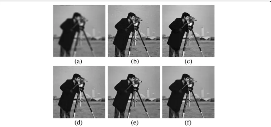
Fig. 6Experiments on the blurry and noisy image of“Cameraman”(256 × 256). aBlurry and noisy (PSNR = 21.22).bThe local TV [5] (PSNR = 22.45,t = 3.7 s).cGOS_TV [15] (PSNR = 23.09,t = 5.7 s).dThe local/nonlocal TV [26] (PSNR = 24.57,t = 10.5 s).eThe nonlocal TV [8] (PSNR = 25.69, t = 6.3 s).fThe proposed model (PSNR = 27.69,t = 5.2 s)

proposed based on the nonlocal TV and uses a linearized proximal alternating minimization algorithm to improve the efficiency. Our result in Fig. 7f shows higher PSNR and shorter CPU time.

5 Conclusions

In this paper, a novel local and nonlocal total variation combination method has been proposed for image res-toration in WSN. To apply the information properly, the image is divided into two regions by an image smoothing scheme. The local TV term is applied on the salient edges and constant regions, and the nonlocal term is ap-plied on the details. The overlapping group sparsity is adopted as a priori constraint term in the proposed model to alleviate the staircase effect as much as pos-sible. To improve the efficiency, we optimize the energy function by the ADMM algorithm, which has complex formulas but is easy to be programmed. Parameter selec-tion criterion for two key parameters is discussed by nu-merical experiments, and it is the other main contribution. By comparing with other state-of-the-art methods, it can be concluded that our method achieves higher efficiency and makes a good balance between alleviating staircase effects and preserving image details.

Acknowledgements

We thank the reviewer for helping us to improve this paper. This work is supported by the National Science Foundation of China (Grant No.61501328) and Doctoral Found of Tianjin Normal University (Grant No.52XB1406).

Funding

Funding was from the National Science Foundation of China (Grant No.61501328) and Doctoral Found of Tianjin Normal University (Grant No.52XB1406).

Authors’contributions

MS proposes the innovation ideas and theoretical analysis, and LF carries out experiments and data analysis.

Consent for publication

Written informed consent was obtained from the patient for the publication of this report and any accompanying images.

Competing interests

The authors declare that they have no competing interests.

Publisher’s Note

Springer Nature remains neutral with regard to jurisdictional claims in published maps and institutional affiliations.

Author details

1_{Tianjin Key Laboratory of Wireless Mobile Communications and Power} Transmission, Tianjin Normal University, Tianjin 300387, China.2College of Electronic and Communication Engineering, Tianjin Normal University, Tianjin 300387, China.3China North Vehicle Research Institute, Beijing 100072, China.

Received: 13 July 2017 Accepted: 27 September 2017

References

1. Q Liang, X Cheng, SC Huang, D Chen, Opportunistic sensing in wireless sensor networks: theory and application. IEEE Trans. Comput.63(8), 2002–2010 (2014)

2. F Zhao, L Wei, H Chen, Optimal time allocation for wireless information and power transfer in wireless powered communication systems. IEEE T. Veh. Technol65(3), 1830–1835 (2016)

3. F Zhao, H Nie, H Chen, Group buying spectrum auction algorithm for fractional frequency reuses cognitive cellular systems. Ad Hoc Netw.58, 239_–246 (2017)

4. F Zhao, W Wang, H Chen, Q Zhang, Interference alignment and game-theoretic power allocation in MIMO heterogeneous sensor networks communications. Signal Process.126, 173–179 (2016)

5. L Mysaker, XC Tai, Iterative image restoration combining total variation minimization and a second-order functional. Int. J. Comput. Vis.66(1), 5–18 (2006) 6. D Chen, L Cheng, Alternative minimisation algorithm for non-local total

variational image deblurring. IET Image Process.4(5), 353–364 (2010) 7. F Rousseau, A non-local approach for image super-resolution using

intermodality priors. Med. Image Anal.14(4), 594–605 (2010)

8. S Yun, H Woo, Linearized proximal alternating minimization algorithm for motion deblurring by nonlocal regularization. Pattern Recogn.44(6), 1312_–1326 (2011)

9. DH Jiang, X Tan, YQ Liang, et al., A new nonlocal variational bi-regularized image restoration model via split Bregman method. EURASIP J. Image Vide

1, 1–10 (2015)

10. J Liu, TZ Huang, XG Lv, et al., High-order total variation-based Poissonian image deconvolution with spatially adapted regularization parameter. Appl. Math. Model.45, 516–529 (2017)

11. M Zhu, T Chan,An efficient primal-dual hybrid gradient algorithm for total variation image restoration(Ucla Cam Report, 2008)

12. X Zhang, M Burger, S Osher, A unified primal-dual algorithm framework based on Bregman iteration. J. Sci. Comput.46(1), 20–46 (2011)

13. S Bonettini, V Ruggiero, On the convergence of primal–dual hybrid gradient algorithms for total variation image restoration. J. Math. Imaging Vis44(3), 236–253 (2012)

14. ZJ Bai, D Cassani, M Donatelli, et al., A fast alternating minimization algorithm for total variation deblurring without boundary artifacts. J. Math. Anal. Appl.415(1), 373_–393 (2014)

15. J Liu, TZ Huang, IW Selesnick, et al., Image restoration using total variation with overlapping group sparsity. Inform. Sciences295(C), 232–246 (2015) 16. G Gilboa, S Osher, Nonlocal operators with applications to image

processing. Multiscale Model. Sim7(3), 1005_–1028 (2008)

17. W Dong, L Zhang, G Shi, et al., Image deblurring and super-resolution by adaptive sparse domain selection and adaptive regularization. IEEE T. Image Process20(7), 1838–1857 (2011)

18. WZ Shao, HS Deng, Q Ge, et al., Regularized motion blur-kernel estimation with adaptive sparse image prior learning. Pattern Recogni51, 402–424 (2016) 19. MS Almeida, M Figueiredo, Deconvolving images with unknown boundaries

using the alternating direction method of multipliers. IEEE T. Image Process

22(8), 3074_–3086 (2013)

20. I Daubechies, M Defrise, CD Mol, An iterative thresholding algorithm for linear inverse problems with a sparsity constraint. Commun. Pur. Appl. Math

57(11), 1413–1457 (2004)

21. SJ Wright, RD Nowak, M Figueiredo, et al., Sparse reconstruction by separable approximation. IEEE Press57(7), 2479–2493 (2009) 22. W Deng, W Yin, On the global and linear convergence of the generalized

alternating direction method of multipliers. J. Sci. Comput.66(3), 889–916 (2016) 23. B He, H Yang, Some convergence properties of a method of multipliers for

linearly constrained monotone variational inequalities. Oper. Res. Lett.23(3), 151–161 (1998)

24. J Eckstein, DP Bertsekas, On the Douglas-Rachford splitting method and the proximal point algorithm for maximal monotone operators. Math. Program.

55(1–3), 293–318 (1992)

25. L Xu, C Lu, Y Xu, J Jia, Image smoothing via L0 gradient minimization. Acm T.Graphic30(6), 1–12 (2011)

26. S Tang, W Gong, W Li, et al., Non-blind image deblurring method by local and nonlocal total variation models. Signal Process.94(1), 339–349 (2014) 27. M Shi, T Han, S Liu, Total variation image restoration using hyper-Laplacian

prior with overlapping group sparsity. Signal Process.126, 65–76 (2015) 28. X Zhang, M Burger, X Bresson, et al., Bregmanized nonlocal regularization