Multistability and bifurcations in a 5D segmented disc dynamo with a curve of equilibria

R E S E A R C H

Open Access

Multistability and bifurcations in a 5D

segmented disc dynamo with a curve of

equilibria

Jianghong Bao

_{and Yongjian Liu}

*_{Correspondence:} majhbao@yahoo.com 1_{School of Mathematics, South}

China University of Technology, Guangzhou, P.R. China

2_{Guangxi Colleges and Universities}

Key Laboratory of Complex System Optimization and Big Data Processing, Yulin Normal University, Yulin, P.R. China

Abstract

Multistability, i.e., coexisting attractors, is one of the most exciting phenomena in dynamical systems. This paper presents a new category of coexisting hidden attractor: five-dimensional (5D) systems with a curve of equilibria. Based on the segmented disc dynamo, a new 5D hyperchaotic system is proposed. The paper studies not only coexisting self-excited attractors but also coexisting hidden attractors in the new system with four types of equilibria: a curve of equilibria, a line equilibrium, a stable equilibrium, and no equilibria. Furthermore, the paper proves that the degenerate Hopf and pitchfork bifurcations occur in the system. Numerical simulations demonstrate the emergence of the two bifurcations.

Keywords: 5D segmented disc dynamo; Curve of equilibria; Multistability; Degenerate Hopf bifurcation; Pitchfork bifurcation

1 Introduction

Multistability or coexisting different attractors for a given set of parameters is one of the most exciting phenomena in dynamical systems [1]. Complex dynamical systems, ranging from human brain, climate, ecosystems to financial markets and engineering applications, typically have many coexisting attractors [2,3]. High dimensional hyperchaotic systems describe natural phenomena more explicitly than low dimensional systems [4]. Nowadays the research of high dimensional multistability systems has captured attention of scientists from around the world.

Recently, it has been shown that multistability is connected with the occurrence of un-predictable attractors which have been called hidden attractors. Hidden attractors may cause disastrous events, such as sudden climate changes, serious diseases, financial crises, etc. [2,5–7]. They are often related to dynamical systems with stable equilibria [8,9], no equilibria [10, 11], a line equilibrium [12,13], or a curve of equilibria [14–17]. A self-excited attractor has a basin of attraction associated with an unstable equilibrium. The classical attractors of Lorenz, Rössler, Chua, Chen, Sprott systems (cases B to S) are those excited from unstable equilibria [16]. This paper presents a new category of hidden attrac-tor: five-dimensional (5D) systems with a curve of equilibria.

For the past few years, many dynamical systems have been reported to study curve-shaped equilibria [14–17]. Table 1 in Ref. [15] classifies the chaotic systems with an infinite

number of equilibria. However, it is noted that no 5D hyperchaotic systems with a curve of equilibria are reported in the literature.

Motivated by the above findings, the paper proposes a new 5D hyperchaotic system based on the segmented disc dynamo. We study not only coexisting self-excited attractors but also coexisting hidden attractors in the new system with four types of equilibria: a curve of equilibria, a line equilibrium, a stable equilibrium, and no equilibria. Further, we study the degenerate Hopf bifurcation and pitchfork bifurcation of the system by bifurca-tion theory [18,19]. Numerical investigations are performed to verify the corresponding theoretical results for the two bifurcations.

The paper is organized as follows. Section2introduces a new 5D segmented disc dy-namo with a curve of equilibria. Section3investigates different types of coexisting at-tractors. Section4investigates the degenerate Hopf bifurcation, and Sect.5analyzes the pitchfork bifurcation. Section6concludes the paper.

2 5D segmented disc dynamo with a curve of equilibria

2.1 Presentation of a 5D segmented disc dynamo with a curve of equilibria

Moffatt proposed the segmented disc dynamo which included the current associated with the radial diffusion of the magnetic field and satisfied the Alfven theorem of flux conser-vation [20]:

⎧ ⎪ ⎪ ⎨ ⎪ ⎪ ⎩

˙

x(t) =r(y–x),

˙

y(t) =mx– (1 +m)y+xz,

˙

z(t) =g(mx2_{+ 1 – (1 +m)xy).}

(2.1)

Based on (2.1), we translateztoz–mand introduce new parameters, which result in the following 5D segmented disc dynamo:

⎧ ⎪ ⎪ ⎪ ⎪ ⎪ ⎪ ⎪ ⎪ ⎨ ⎪ ⎪ ⎪ ⎪ ⎪ ⎪ ⎪ ⎪ ⎩

˙

x(t) =r(y–x),

˙

y(t) =xz– (1 +m)y+v,

˙

z(t) =g(mx2_{+ 1 – (1 +m)xy) –k}

1u+k6z,

˙

u(t) =k2y2–k3z,

˙

v(t) =k4x–xz+k5v,

(2.2)

whererandmare positive parameters, and the others are real parameters.

The divergence of the system is∇ ·V= –r– 1 –m+k5+k6, and the system is dissipative if k5+k6<r+m+ 1. System (2.2) is invariant under the transformation (x,y,z,u,v)→ (–x, –y,z,u, –v).

Now in order to obtain the hyperchaos with three positive Lyapunov exponents (LEs), we need to exclude some parameter sets that cannot make system (2.2) show bounded chaotic solutions.

Theorem 2.1 If the following conditions are satisfied:

g=k2= 0, k1=k3–k6=r–k4= –1 –k5=m+ 1 –r< 0, (2.3)

Figure 1Parameters (g,k1,k2,k3,k4,k5,k6) = (0, 0.05,

1, –0.6, 10, –1, 0), initial condition

(–2, 7.9221, –1, 0, 15), regions of various dynamical behaviors for the parametersmandr. Chaos with one positive LE in purple; Hyperchaotic regions with two positive LEs in green; Hyperchaotic regions with three positive LEs in black; Point regions with five negative LEs in red

Proof From system (2.2), we can get

˙

x+˙y+˙z+u˙+v˙= (k4–r)x– (m+ 1 –r)y– (k3–k6)z–k1u+ (k5+ 1)v. (2.4)

By condition (2.3), Eq. (2.4) becomes

˙

x+˙y+˙z+u˙+v˙= (k4–r)(x+y+z+u+v).

Hence

x(t) +y(t) +z(t) +u(t) +v(t) =ce(k4–r)t_,

wherecis an arbitrary constant. Fork4–r> 0, system (2.1) is not chaotic because at least one ofx(t),y(t),z(t),u(t), andv(t) is not bounded.

Figure1shows the regions of various dynamical behaviors in the space of the param-eters (m,r)∈[1, 10]×[50, 60] with the other fixed parameters (g,k1,k2,k3,k4,k5,k6) = (0, 0.05, 1, –0.6, 10, –1, 0) and the initial condition (–2, 7.9221, –1, 0, 15). Chaotic and

hy-perchaotic regions also include hidden chaos and hyperchaos.

2.2 Equilibria and stability

Fork4= 1 +m,k5= –1, andk1k3= 0, system (2.2) has a curve of equilibria

E1

x,x,k2 k3

x2,gk3(1 –x 2_{) +k}

2k6x2

k1k3

, (1 +m)x–k2 k3

x3

.

We first discuss the case:k4= 1 +mandk5= –1. Fork1k3= 0, there is an equilibrium

E2(0, 0, 0,_kg₁, 0). Fork1= 0 andg= 0, there is no equilibria. Fork1=g= 0 ork3= 0, the sys-tem always has a line equilibrium. The other case,k4= 1 +mandk5= –1, can be similarly discussed.

Let

S1=

(m,g,k1,k2,k3,k4,k5,k6)

g=k2= 0,k1k3= 0,k4= 1 +m,

k5= –1,k6< 0

,

S2={(m,k1,k3,k4,k5,k6)|k1k3= 0,k4= 1 +m,k5< –1,k6< 0},

Theorem 2.2

(1) Suppose(m,g,k1,k2,k3,k4,k5,k6)∈S1.Ifk1k3> 0,then the equilibriumE1of system

(2.2)has at least three-dimensional stable manifold and one-dimensional unstable manifold.Otherwise,E1has at least four-dimensional stable manifold.

(2) Suppose(m,k1,k3,k4,k5,k6)∈S2.Ifk1k3> 0,then the equilibriumE2is unstable and

has four-dimensional stable manifold and one-dimensional unstable manifold. Otherwise,E2is stable and has five-dimensional stable manifold.

3 Multistability

The complex dynamics of a hyperchaotic system are usually produced by the bifurcations at equilibria. However, curve-shaped equilibria are non-isolated and non-hyperbolic, so it is difficult to obtain the complex dynamics due to the bifurcation at equilibria. The meth-ods of numerical analysis are vital for these systems with a curve of equilibria [14]. In addition, lots of other complex dynamics of system (2.2) are also discovered by means of the detailed numerical analysis.

3.1 Coexisting chaos and hyperchaos for system (2.2) with a curve of equilibria

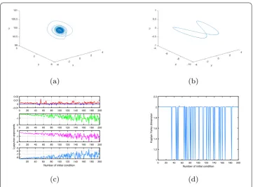
When (m,r,g,k1,k2,k3,k4,k5,k6) = (99, 9, 5, –10, 10, 10, 100, –1, 0), system (2.2) has a curve of equilibria (x,x,x2_,1

2(x

2_{– 1), 100x(1 –x}2_{)). For the initial condition (–2, 7.9221, –1, 0,}

15.8407), system (2.2) has the LEs (0.0095, 0.0017, 0, –10.5037, –22.3829), and the Kaplan– Yorke dimension is 3.0011. For the initial condition (0.7513, 0.2551, 0.5060, 0.6991, 0.8909), the LEs are (0.0038, 0, –0.0151, –10.1246, –17.2288), and the Kaplan–Yorke dimension is 2.2517. The hyperchaotic and chaotic attractors are shown in Fig.2. Figure2(c) shows the LEs spectrum with 200 varied initial conditions, and Fig.2(d) shows the LEs spectrum for r∈[7, 50] and the initial condition (–2, 7.9221, –1, 0, 15.8407).

3.2 Coexisting chaos and hyperchaos for system (2.2) with no equilibria

When (m,r,g,k1,k2,k3,k4,k5,k6) = (0.11, 8, 1.2, 0, 10, 0, –100, –1, 0), system (2.2) has no equilibria. For the initial condition (–7.4047, –10.8076, 8.9184, –0.4523, 0.0641), the sys-tem has the LEs (0.0062, 0, –0.0090, –0.0133, –10.0797), and the Kaplan–Yorke dimension is 2.6889. The chaos is shown in Fig.3(a), and Fig.3(b) shows the Poincaré map. For the initial condition (–2, 0, 0.1, 0.1, 0), system (2.2) has the LEs (0.0032, 0.0018, 0, –0.0123, –10.0995), and the Kaplan–Yorke dimension is 3.4065. A hyperchaotic attractor is shown in Fig.3(c), and Fig.3(d) shows the Poincaré map. Figure3(e) shows the LEs spectrum with 200 varied initial conditions, and the corresponding Kaplan–Yorke dimensions are shown in Fig.3(f ).

3.3 Coexisting chaotic, quasiperiodic and periodic attractors for system (2.2) with a line equilibrium

Figure 2Parameters (m,r,g,k1,k2,k3,k4,k5,k6) = (99, 9, 5, –10, 10, 10, 100, –1, 0); (a) chaotic attractor;

(b) hyperchaotic attractor; (c) Lyapunov exponents spectrum with 200 varied initial conditions; (d) Lyapunov exponents spectrum forr_∈[7, 50] and initial condition (–2, 7.9221, –1, 0, 15.8407)

3.4 Coexisting chaos and hyperchaos for system (2.2) with a stable equilibrium

When (m,r,g,k1,k2,k3,k4,k5,k6) = (1.3, 1, 0.12, 0.01, 0, –0.001, –1, 0, –0.001), system (2.2) has a stable equilibrium (0, 0, 0, 12, 0). For the initial condition (0.0326, 0.5612, 0.8819, 0.6692, 0.1904), the LEs are (0.0031, 0, –0.0172, –0.0143, –3.2647). The chaotic attractor is shown in Fig. 5(a), and Fig.5(b) shows the Poincaré map. For the initial condition (0, 0, 0, 0, 0), the LEs are (1.8956, 1.4008, 0, –0.0015, –6.5956), and the system displays hy-perchaos.

3.5 Coexisting self-excited attractors

When (m,r,g,k1,k2,k3,k4,k5,k6) = (1.3, 1, 12, 0.01, –0.1, –0.001, –2.3, –1, 0.1), system (2.2) has an unstable equilibrium (0, 0, 0, 1200, 0). For the initial condition (–0.3394, –64.0648, 91.0435, –75.5546, 10.5920), system (2.2) has the LEs (0.0082, 0.0056, 0, –0.5393, –3.5561). A hyperchaotic attractor is obtained (see Fig. 6(a)), and the Poincaré map is shown in Fig. 6(b). For the initial condition (0.1576, 0.9706, 0.9572, 0.4854, 0.8003), the system has the LEs (0.0047, 0, –0.1228, –0.5298, –3.5469). The chaotic attractor is obtained in Fig.6(c). The Poincaré map is shown in Fig.6(d). Whenr∈[1, 10], Fig.7(a) shows the LEs spectrum, and the corresponding bifurcation diagram is shown in Fig.7(b).

4 Degenerate Hopf bifurcation in system (2.2)

Figure 3Parameters (m,r,g,k1,k2,k3,k4,k5,k6) = (0.11, 8, 1.2, 0, 10, 0, –100, –1, 0); (a) chaotic attractor;

(b) Poincaré map of the chaotic attractor; (c) hyperchaotic attractor; (d) Poincaré map of the hyperchaotic attractor; (e) Lyapunov exponents spectrum with 200 varied initial conditions; (e) Kaplan–Yorke dimension

Let

ω=–k1k3,

S=

(m,r,g,k1,k2,k3,k4,k5)

m> 0,r> 0,k2=k5= 0,k1k3< 0,

g= 0, –(m+ 1)(r+m+ 1) <k4< 0

.

For (m,r,g,k1,k2,k3,k4,k5)∈S, system (2.2) has only one equilibriumE2(0, 0, 0,_kg₁, 0).

E2has the eigenvaluesλ(k6) = k6±

√

4k1k3+k62

2 , and the other eigenvalues ofE2satisfy

Figure 4Parameters (m,r,g,k1,k2,k3,k4,k5,k6) = (1.1, 6.1, 12, 0.1, 0, 0, –100, –1, 0); (a) chaos; (b) period;

(c) Lyapunov exponents spectrum with 200 varied initial conditions; (d) Kaplan–Yorke dimension

Figure 5Parameters (m,r,g,k1,k2,k3,k4,k5,k6) = (1.3, 1, 0.12, 0.01, 0, –0.001, –1, 0, –0.001); (a) Chaotic attractor;

(b) Poincaré map of the chaotic attractor

According to the Routh–Hurwitz criterion, the real parts of the rootsλare negative if and only if

1=m+r+ 1 > 0,

2=r

(m+ 1)(r+m+ 1) +k4

> 0,

3= –rk42> 0.

Figure 6Parameters (m,r,g,k1,k2,k3,k4,k5,k6) = (1.3, 1, 12, 0.01, –0.1, –0.001, –2.3, –1, 0.1); (a) hyperchaotic

attractor; (b) Poincaré map of the hyperchaotic attractor; (c) chaotic attractor; (d) Poincaré map of the chaotic attractor

Figure 7Initial condition (0.1576, 0.9706, 0.9572, 0.4854, 0.8003), parameters

(m,g,k1,k2,k3,k4,k5,k6) = (1.3, 12, 0.01, –0.1, –0.001, –2.3, –1, 0.1) andr∈[1, 10]; (a) Lyapunov exponents

spectrum; (b) bifurcation diagram

The transversality condition

Re

dλ(k6)

dk6

k6=0 =1

2> 0 (4.1)

Theorem 4.1 Considering system (2.2), for parameter (m,r,g,k1,k2,k3,k4,k5)∈S and

Proof By the changes

⎧

From (4.1), the transversality condition holds. Now we calculate the Lyapunov coeffi-cients, which show the stability of the equilibrium and the periodic orbit which appears.

h31=

3(2ω+i)ωr f(2) ,

3i(2ω–ir)(2ω+i)ω

f(2) , 0, 0,

3iω(–4ω2+ 2i(m+r+ 1)ω+r(m+ 1 –k4))

f(2)

,

H32=

6ω2_rb

f(2)(2iω+ 1 +m)(2iω+r)(0, 1, 0, 0, –1),

G32= 0,

where

X= (x1,x2,x3,x4,x5), Y= (y1,y2,y3,y4,y5),

f(n) = –n3ω3i–n2(m+r+ 1)ω2+nr(m+ 1)ωi–k4r.

Therefore

l1= 1

2Re(G21) = 0, l2= 1

12Re(G32) = 0.

Sincel1=l2= 0, we continue to calculatel3. Some vector expressions are too complex, and for the convenience of expression, we write the results after calculation as follows:

B(h11,h32) =B(h20,h¯32) =B(h¯20,h41) =B(h21,h22) =B(h30,h¯31)

=B(h¯30,h40) =B(q,h33) = (0, 0, 0, 0, 0),

B(h21,h31) =

–3b

f(2)(2iω+ 1 +m)(2iω+r)

0,k1r,gω

(m+ 1)ω– 2ri, 0,ω 2_r

k3

,

B(q¯,h42) =

4(2ω+i)rω2i k3f(3)f(2)2

(0, –c, 0, 0,c),

where

b= –8iω3– 4(m+r)ω2+ 2i(mr–m– 1)ω–r(m+ 1),

c= 216(k3+ 3)ω6– 180i(k3+ 3)(1 +m+r)ω5

– 66(m+ 1) + 25r(m+ 1)(k3+ 3) + 18r2

ω4

+ 5ir6(m+ 2)(m+r) – 7k4+ 6

(k3+ 3) – 18r

ω3

+r6mr(m+ 2) – 13k4(m+r+ 1)

(k3+ 3) + 18r

ω2

+ 5k4(k3+ 3)(1 +m)r2ωi–k42r2(k3+ 3).

Hence one hasl3= –4g((m+2)(m+1)+r(m–3))ω

4_+g(4r2_{(m+2)+r(m+1)(k}

4–m+3))ω2+gk4r2

4(64ω6+16((m+1)2+r2_)ω4_+4((m+1)2_r2_+2k

4r(m+1+r))ω2+k42r2) .

Numerical simulation Form=r=g= 1,k2=k5= 0,k1= –0.001,k3= 0.001,k4= –5, and

Figure 8Phase portraits of system (2.2) for initial condition (1, 0, 1, 0, 0) and parameters (m,r,g,k1,k2,k3,k4,k5,k6) = (1, 1, 1, –0.001, 0, 0.001, –5, 0, 0.001)

5 Pitchfork bifurcation in system (2.2)

We utilize the center manifold theorem and the bifurcation theory [18,19] to study pitch-fork bifurcation of system (2.2).

Let

S={(k1,k2,k3,k4,k5,k6)|k4=k5=k6= 0,k1k3> 0,k2k3> 0}.

When (k1,k2,k3,k4,k5,k6)∈S, system (2.2) has only one equilibriumE2(0, 0, 0,_kg₁, 0). By the changes (4.2), system (2.2) becomes the following system (still denoted byx,y,z, u,v):

⎧ ⎪ ⎪ ⎪ ⎪ ⎪ ⎪ ⎪ ⎪ ⎨ ⎪ ⎪ ⎪ ⎪ ⎪ ⎪ ⎪ ⎪ ⎩

˙

x(t) =r(y–x),

˙

y(t) =xz– (m+ 1)y+v,

˙

z(t) =g(mx2_{– (1 +m)xy) –k} 1u,

˙

u(t) =k2y2–k3z,

˙

v(t) =k4x–xz,

(5.1)

and the equilibriumE2is moved toO(0, 0, 0, 0, 0). The Jacobian matrix atOis

J=

⎛ ⎜ ⎜ ⎜ ⎜ ⎜ ⎜ ⎝

–r r 0 0 0

0 –m– 1 0 0 1

0 0 0 –k1 0

0 0 –k3 0 0

0 0 0 0 0

⎞ ⎟ ⎟ ⎟ ⎟ ⎟ ⎟ ⎠

,

and the corresponding characteristic equation is

λ3+ (m+r+ 1)λ2+ (mr+r)λλ2–k1k3

= 0.

System (2.2) has a zero eigenvalueλ1= 0 and the other four eigenvalues

λ2= –r, λ3= –(m+ 1), λ4,5=±

k1k3.

Theorem 5.1 For(k1,k2,k3,k4,k5,k6)∈S,system(2.2)undergoes a pitchfork bifurcation

at E2(0, 0, 0,_kg₁, 0).Furthermore,when k4< 0,there is only one equilibrium E2which is

sta-ble near the left-hand side of k4= 0;when k4> 0,E2becomes unstable and the other two

equilibria are stable near the right-hand side of k4= 0.

Proof The corresponding eigenvectors are

From the center manifold theorem, there exists a center manifold for Eqs. (5.3), which can be expressed locally as the following set through the variablex1andε:

Wc(0) =

whereδandδ¯are sufficiently small. Assume that

Consideringε˙≡0, the center manifold should satisfy

Figure 9Pitchfork bifurcation diagram in system (2.2) neark4= 0

Applying Eqs. (5.6) intox˙1=g1of (5.3) and reducing the vector field to the center man-ifold, we can get

⎧ ⎨ ⎩

˙

x1=F(x1,ε) +o(4),

˙

ε= 0, (5.7)

where

F(x1,ε) =

(r(m+ 1)2– (m+r+ 1)ε)(k3(m+ 1)2ε–k2x12)x1

k3r(1 +m)5

. (5.8)

F(x1,ε) satisfies

⎧ ⎪ ⎪ ⎪ ⎨ ⎪ ⎪ ⎪ ⎩

F(0, 0) = 0, ∂F

∂x1|(0,0)= 0,

∂F

∂ε|(0,0)= 0, ∂2F

∂x12|(0,0)= 0,

∂2F

∂x1∂ε|(0,0)=

1 1+m= 0,

∂3F

∂x13|(0,0)= –

6k2

(1+m)3_k 3 = 0,

which indicates that the equilibrium (x1,ε) = (0, 0) of Eqs. (5.7) undergoes a pitchfork bi-furcation atε= 0 (k4= 0). Since –∂

3_F

∂x13/

∂2F

∂x1∂ε> 0, the bifurcation direction is near the

right-hand side ofε= 0 (k4= 0). So Theorem5.1is proved.

Numerical simulation Forr=m=k1=k2=k3= 1 andg=k5=k6= 0, (5.8) becomes

F(x1,ε) = 1

32(4 – 3ε)

4ε–x12

x1.

As shown in Fig.9, system (2.2) undergoes a pitchfork bifurcation, which accords with Theorem5.1.

6 Conclusions

LEs is also displayed. Besides, by choosing an appropriate bifurcation parameter, the paper proves that the degenerate Hopf bifurcation and pitchfork bifurcation occur in the system. The simulation results demonstrate the correctness of the two bifurcations analysis.

The research on the new system may enrich the hyperchaotic theories and engineering applications. It is also hoped that the work is helpful to identify the geometrical charac-teristics of lower dimensional chaotic attractors. More studies will be explored to reveal the riddled property of the basin of attraction of the hyperchaotic attractors.

Acknowledgements

The authors would like to express many thanks to Professor Yuming Chen for his corrections and comments on this manuscript.

Funding

The research is supported by the Open Project of Guangxi Colleges and Universities Key Laboratory of Complex System Optimization and Big Data Processing (No. 2017CSOBDP0303) and the National Natural Science Foundation of China (No. 11671149).

Competing interests

The authors declare that they have no competing interests.

Authors’ contributions

The authors have made the same contribution. All authors read and approved the final manuscript.

Publisher’s Note

Springer Nature remains neutral with regard to jurisdictional claims in published maps and institutional affiliations.

Received: 20 November 2018 Accepted: 6 August 2019

References

1. Pisarchik, A.N., Feudel, U.: Control of multistability. Phys. Rep.540, 167–218 (2014)

2. Dudkowskia, D., Jafari, S., Kapitaniak, T., Kuznetsov, N.V., Leonovc, G.A., Prasad, A.: Hidden attractors in dynamical systems. Phys. Rep.637, 1–50 (2016)

3. Liu, Y., Li, J., Wei, Z., Moroz, I.: Bifurcation analysis and integrability in the segmented disc dynamo with mechanical friction. Adv. Differ. Equ.2018, 210 (2018)

4. Ojoniyi, O.S., Njah, A.N.: A 5D hyperchaotic Sprott B system with coexisting hidden attractors. Chaos Solitons Fractals

87, 172–181 (2016)

5. Abdel-Gawad, H.I., Saad, K.M.: On the behaviour of solutions of the two-cell cubic autocatalator reaction model. ANZIAM J.44, E1–E32 (2002)

6. Abdel-Gawad, H.I., Saad, K.M.: A chemotherapy-diffusion model for the cancer treatment and initial dose control. Kyungpook Math. J.48, 395–410 (2008)

7. Saad, K.M., Iyiola, O.S., Agarwal, P.: An effective homotopy analysis method to solve the cubic isothermal auto-catalytic chemical system. AIMS Math.3(1), 183–194 (2018)

8. Molaie, M., Jafari, S., Sprott, J.C., Golpayegani, S.M.R.H.: Simple chaotic flows with one stable equilibrium. Int. J. Bifurc. Chaos Appl. Sci. Eng.23, 1350188 (2013)

9. Wang, X., Chen, G.: A chaotic system with only one stable equilibrium. Commun. Nonlinear Sci. Numer. Simul.17, 1264–1272 (2012)

10. Pham, V.T., Volos, C., Jafari, S., Kapitaniak, T.: Coexistence of hidden chaotic attractors in a novel no-equilibrium system. Nonlinear Dyn.87, 2001–2010 (2017)

11. Jafari, S., Sprott, J.C., Golpayegani, S.M.R.H.: Elementary quadratic chaotic flows with no equilibria. Phys. Lett. A377, 699–702 (2013)

12. Jafari, S., Sprott, J.C.: Simple chaotic flows with a line equilibrium. Chaos Solitons Fractals57, 79–84 (2013) 13. Li, Q.D., Hu, S.Y., Tang, S., Zeng, G.: Hyperchaos and horseshoe in a 4D memristive system with a line of equilibria and

its implementation. Int. J. Circuit Theory Appl.42, 1172–1188 (2014)

14. Chen, Y., Yang, Q.: A new Lorenz-type hyperchaotic system with a curve of equilibria. Math. Comput. Simul.112, 40–55 (2015)

15. Singh, J.P., Roy, B.K., Jafari, S.: New family of 4-D hyperchaotic and chaotic systems with quadric surfaces of equilibria. Chaos Solitons Fractals106, 243–257 (2018)

16. Barati, K., Jafari, S., Sprott, J.C., Pham, V.T.: Simple chaotic flows with a curve of equilibria. Int. J. Bifurc. Chaos Appl. Sci. Eng.26, 1630034 (2016)

17. Gotthans, T., Petr˘zela, J.: New class of chaotic systems with circular equilibrium. Nonlinear Dyn.81, 1143–1149 (2015) 18. Kuznetsov, Y.A.: Elements of Applied Bifurcation Theory. Springer, New York (1998)

19. Wiggins, S.: Introduction to Applied Nonlinear Dynamical Systems and Chaos. Springer, New York (1990) 20. Moffatt, H.K.: A self consistent treatment of simple dynamo systems. Geophys. Astrophys. Fluid Dyn.14, 147–166