Topographic optimal network design of the unified control points in Korea
Tae-Suk Bae1, Jay Hyoun Kwon2, and Chang-Ki Hong3
1Department of Geoinformation Engineering, Sejong University, 98 Gunja-dong, Gwangjin-gu, Seoul 143-747, Korea 2Department of Geoinformatics, University of Seoul, 90 Jennong-dong Dongdaemun-Gu, Seoul 130-743, Korea
3Department of Satellite Geoinformatics Engineering, Kyungil University, 33 Buho-ri, Hayang-eup, Gyeongsan-si, Gyeongsangbuk-do 712-701, Korea
(Received April 21, 2009; Revised December 7, 2010; Accepted February 11, 2011; Online published June 21, 2011)
In general, the geometric approach based on the criterion matrix has focused on the optimal network design. At the scale of the local area, however, the topographic undulations should be considered for ground applications, such as geoid determination. Since the multi-purpose uni ed control points (UCPs) are planned for providing gravimetric information as well as the three-dimensional positions, the effect of high-frequency signals from topography need to be considered in the network optimization process. In this study, an optimization procedure incorporating the geometric and topographic con guration is presented. A Digital Elevation Model (DEM) that represents terrain information is combined with the second-order design algorithm with Taylor-Karman structure. The smoothed DEM data are removed from the original dataset, resulting in high-frequency data only; the root mean squares of the residuals are computed to create the weight matrix. As a result, the directional pattern is clearly seen in the weight matrix, and the nal location of the network shows the north-south directional properties. Once the network selection process is complete, the Minimum Spanning Tree (MST) is created to examine the distribution of the baselines. The statistics on the MST were used for the criterion of optimal network validation.
Key words:Optimal network, Taylor-Karman structure, uni ed control point.
1.
Introduction
Network optimization problem has been a popular is-sue in geodetic applications, especially in establishing new tracking or control stations. The well-known approach of optimal network design is to use the criterion matrix that is homogeneous and isotropic (Grafarend and Schaffrin, 1979; Schaffrin, 1985). This method is based on the ge-ometric con guration of the candidate stations, i.e., either scattered or regularly gridded; thus, its nal network is affected by only geometric relations between candidates. Without exception, however, the network stations are built on the physical surface of the Earth, which is closely con-nected with the topographic condition.
In 2007, the Korean government initiated a campaign to establish newly designed national control points. The con-trol points, which are called uni ed concon-trol points (UCPs), are supposed to contain not only the traditional position in-formation but also gravimetric inin-formation, such as gravity anomaly and geoidal height. The rationale for this cam-paign is to support scienti c and engineering applications by providing all of the necessary information at common points. In fact, future plans are to expand the information at UCPs based on the various demands of users. For example, data on weather or environmental information can be added as contents provided at UCPs so that researchers can use
Copyright cThe Society of Geomagnetism and Earth, Planetary and Space Sci-ences (SGEPSS); The Seismological Society of Japan; The Volcanological Society of Japan; The Geodetic Society of Japan; The Japanese Society for Planetary Sci-ences; TERRAPUB.
doi:10.5047/eps.2011.02.007
and analyze the various data provided at common points. The current question revolves around the optimal distribu-tion for the UCP networks. As the UCPs contain geometric and physical information, variations in topography and the geometric con guration have to be considered at the same time.
The primary aim of this study was to develop an opti-mal network design algorithm that considers both geomet-ric and physical circumstances. Here, the geometgeomet-ric con-sideration is the traditional concept, namely, the weighting scheme based on the relative distances of points or stations. The physical consideration, on the other hand, involves the effect of topography, which could be crucial in collecting physical quantity such as gravity measurement. In other words, the network should be distributed in such a way that it can sense necessary frequency components of the in-tended signal. If the network in a mountainous area is not dense enough, the measured gravity will suffer from alias-ing, which results in excessive amplitude at low frequency by smearing of the high-frequency signal. Therefore, to-pographic information, such as a Digital Elevation Model (DEM), should be used to design a network that is optimal in both geometrical and physical aspects.
The primary component of network optimization is still the geometric relations between stations, and information obtained from the DEM is used to assist the selection algo-rithm in our approach. Combining these components prop-erly to achieve optimal solutions is considered to be a useful step, especially on the local area scale. The high-frequency part of the topography is essential for ground applications
because the gravimetric quantity is likely to be more sen-sitive to the high-frequency signal; thus, high-frequency data were separated from the original DEM to determine the weights for each candidate station. Since there are no explicit criteria to stop the selection process, in this study, we controlled the process using the speci c requirements of the baselines with the Minimum Spanning Tree (MST). As GPS measurements are widely used in such studies, the MST is considered to be a good way to quantify the chosen network.
The algorithms presented in this study are programmed in MATLAB script.
2.
Theory of Network Optimization
The ideal network can be de ned to have a homoge-neous and isotropic variance-covariance matrix, which is called the criterion matrix (Grafarend, 1972). “Homogene-ity” means that it is invariant with respect to a translation, and “Isotropy” refers to its rotational symmetry. Thus, the homogeneous and isotropic ideal network has a uniform quality throughout the network, and the local error ellipses will be circular and equally sized. The criterion matrix can be described by the Taylor-Karman structure, which is de-ned by the variance-covariance matrix between two points in the network. The general form of the 3×3 criterion ma-trix of the Taylor-Karman structure for two points is given by Schaffrin (1985, p. 586) as
σ2
whereri,rjrepresent the coordinates ofPi andPj,
respec-tively, andsindicates the distance between these two points related to the criterion matrix. The directional covariance functions,l(s)andm(s), correspond to the longitudinal
and cross directions, respectively, and the unitless variance component,σ02, is multiplied by the criterion matrix. The desired variance of the estimated coordinates in the network conforms to the covariance function of zero distance; that is, the case of two identical points. The analytical formula of covariance functions are given by Grafarend and Schaffrin (1979) as
whereK0 and K1 are the modi ed Bessel function of the
second kind, i.e., zero and rst order, respectively. The characteristic distance, d, of the network can be chosen so that the maximum distance of the network is the upper limit of 10d according to Wimmer (1982). Another type of characteristic distance can be found in Schmitt (1980).
From Eq. (1), it is clear that the criterion matrix is not dependent on the measurement types or linear mod-els with speci c rank-de ciency. The second order Design (SOD) was successfully implemented for the network de-sign of ground tracking stations for the Low Earth Orbiter (LEO) orbit determination (Bae, 2005). This approach optimizes the cofactor matrix by determining the mea-surement weights between candidate and network stations. Other approaches, such as zero, rst, and third order de-sign (ZOD/FOD/TOD) can be referred to Schaffrin (1985) and/or Kuang (1996).
The basic idea of the SOD is to minimize the difference between the criterion and cofactor matrix of the estimated point coordinates in the network by estimating the weight for each measurement between two points. The ideal cofac-tor matrix (“criterion” matrix) can be computed from the Taylor-Karman structure, and the cofactor matrix of the es-timated point coordinates are obtained from the design ma-trix of the assumed observation model (distance measure-ments in this study). Let us assume the linearized Gauss-Markov Model (GMM) of
yn×1 =An×mξm×1+en×1, e∼
0, σ02P−1 (4)
with the diagonal weight matrixP, where yand Aare the
n ×1 observation vector and the n ×m design matrix, respectively. The term ξ represents the unknown vector for the point coordinates, and then ×1 random erroreis assumed to have a zero-mean and same variance component as in Eq. (1). Then, the condition equation for SOD can be represented by
Qξˆ −C=min., (5)
where Qξˆ is the cofactor matrix of the estimated points coordinatesξˆgiven by
Qξˆ =ATP A−1 (6)
Without any loss of generality, Eq. (5) can be rewritten as
AT
P A−C−1= min
P:=diagp (7)
The nal solution for the weight components is given by
A C AT ∗A C ATˆp=vecdiagA C AT, (8)
where∗ de nes the Hadamard product of matrices with equal size. For the detailed derivation of the above equation, see Bae (2005).
3.
Digital Elevation Model
Longitude [deg]
Fig. 1. DEM of Korean peninsula (SRTM with the spatial resolutions of 45 and 60 arcseconds for latitude and longitude, respectively).
SRTM is 3 arcseconds, from which the coarse DEM with 45 and 60 arcseconds for latitude and longitude, respectively, are extracted and used in this study. The DEM is restricted to within the range of 34–39◦ of latitude and 126–129.5◦ of longitude, which corresponds to the mainland of South Korea.
As can be seen in Fig. 1, in N-S direction, the Ko-rean peninsula has a long-spanned shape as well as a chain of mountains. The topographic variation reaches up to 1600 m, mostly along the mountain range on the east coast and south-west area. Since the gravity information clearly reflects variations in the terrain, high-frequency compo-nents of the gravity signal mainly appear in the mountain-ous area. Therefore, it is important to assess the weighting criteria for the UCPs based on the terrain. In other words, more stations should be established in mountainous area for gravimetric applications. The approach used in this study is to remove the low-frequency data from the DEM, leaving only the high-frequency part which reflects the topographic information of the area. The low-frequency data can gen-erally be obtained by applying smoothing techniques or a low-pass filter. As the mountain chain in Korea is a pre-dominant component of the N-S direction, we decided on computing the smoothed data along the E-W direction so as to preserve the directional properties. The residuals are then used to compute the weight for each station.
4.
Smoothing Technique
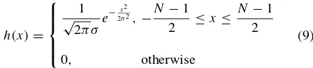
Many smoothing techniques exist, but as discussed ear-lier, the DEM is smoothed along the same latitude using one-dimensional Fourier transform. The smoothing process is regarded as a convolution of the data and a window func-tion (see Eq. (9)). Also, the convolufunc-tion of two signals in
the time domain can be performed in the frequency domain by the convolution theorem, which requires three applica-tions of the Fourier transform. The Fourier transform of the convolution equals the product of the spectra (Fourier transforms) of the convolved functions.
Due to the finite extent of the signal (DEM), a taper func-tion is used to reduce the spectral leakage on the local fre-quencies. The one-dimensional Gaussian filter with a size of 5 pixels smoothes the DEM row-wise (E-W direction), padding two pixels of zero on both ends:
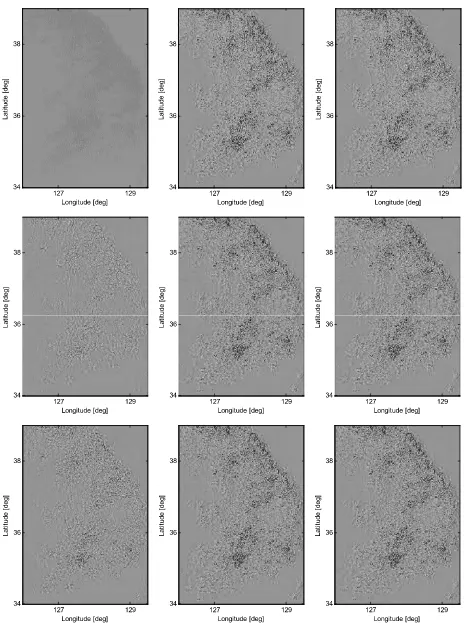
h(x)= ation of the Gaussian distribution, and N is the window size; the values of 0.65 and 5 are used for σ and N, re-spectively. Since each pixel corresponds approximately to 1.5×1.5 km, and the plans are to install UCPs in Korea at 10-km intervals, the window size should not exceed the spacing between UCPs. If the window has a larger size, the DEM is smoothed too much, resulting in exaggerated residuals (Fig. 2). In addition, the smoothing effect of the sigma value shows a tendency to become less for small val-ues (0.45), whereas large valval-ues are highly smoothed (0.85). Since the convolution generates the vector with a dimension that is the sum of two vectors minus 1, both the signal and the filter are padded with zero to match the dimension, be-cause a digital filter is time-invariant (Jekeli, 2007). Then, based on the convolution theorem, fast Fourier transform (FFT) is applied three times to obtain the smoothed DEM.
Figure 2 shows the residuals of DEM after the smoothed data have been removed, revealing a clear illustration of topographic information on Korea. For the weights of each candidate station based on the DEM residuals (high-frequency part), the root mean squares (RMS) of a total of 5 pixels (the pixel for the computation and two pixels on each side of the E-W direction) are calculated. Since the RMS values can range widely, these are normalized row-wise to be on a uniform scale (maximum of 1 for the high-est values at each row). This RMS can then be used for the topographic weight information in determining the network stations. A strong tendency of variation in DEM weighting along the E-W direction can be seen (see Fig. 8) as well as the dominant pattern in the N-S direction, which is closely related to the topographic distribution of Korea.
5.
Selection of Optimal Network
mea-Fig. 2. Residuals after removing the smoothed DEM based on the convolution theorem using one-dimensional Gaussian filter: (Top) Sigma 0.45 (Middle) Sigma 0.65 (Bottom) Sigma 0.85. Each row represents a window size of 5, 10, and 20 (from left), respectively.
surements between already chosen network stations. The criterion matrix at each step is stored to be used again in the following steps. The network station is chosen from the candidate stations to have the most uniform weights to
Fig. 3. Flow chart of the SOD network optimization algorithm (Bae, 2005).
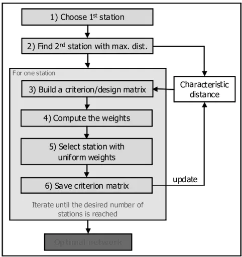
Fig. 4. Flow chart of the optimal network design with the DEM weighting.
be greater than half of the characteristic distance. Figure 3 shows a ow chart of the algorithm for the optimal network selection.
In addition to the above algorithm, it is necessary to in-corporate the topographic information into the network op-timization algorithm to customize for the speci c condi-tions described in this study. Thus, the topographic weight information (see Fig. 8) is used for the selection process. That is, under the geometric condition, the top ten stations with most uniform weight variation are selected, and the station with the highest topographic weight is chosen for the next network station. Details on the algorithm follow in next section.
6.
Test Results
res-127 129
Fig. 5. Candidate stations on a regular grid. The spatial resolution of the grid is 3×2which corresponds to 5×5 km (total 7,451 candidate stations).
olution of 45and 60for latitude and longitude directions, respectively. Consequently, the candidate stations coincide with the DEM at an integer multiple of each pixel. The area of each grid is equivalent to roughly 5×5 km. Since the criterion matrix requires Cartesian coordinates (see Eq. (1)), the DEM should be converted into ellipsoidal heights. The EGM96 geopotential model is used to calculate the geoid undulation, which is combined with the orthometric heights and then transformed into the Cartesian coordinates.
The optimal network selection process begins with two stations of the International Ground Station (IGS) network, SUWN and DAEJ, although these two stations are rather close to each other. The number of stations in the final net-work is dependent on the budget of the project, but this pro-cess can be continued until the baseline length reaches the specified length. The average trace of the cofactor matrix, however, implies that the network may not be improved sig-nificantly over 40 stations.
Figure 6 shows an example of how the network stations are chosen. As can be seen in the figure, the priority of the next network station is scaled 0–1 (1 for most probable candidate); thus, the candidate stations around the current network stations have lower values. This figure shows the case of the 25th network station, which is denoted as a white triangle in lower left area. The next station will be chosen based on the current network distribution.
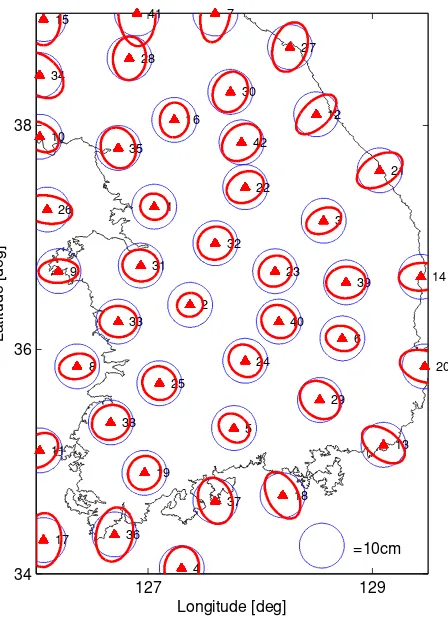
Figure 7 represents the configuration of a total of 42 network stations, starting from two IGS tracking stations,
Longitude [deg]
Fig. 6. Example: The 25th network station of the optimal network (white triangle). The value of 1 represents the top priority for the next network station based on the current network configuration.
127 129
Longitude [deg]
Latitude [deg]
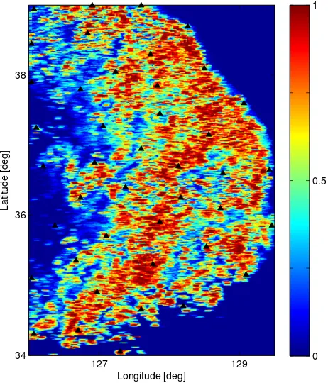
127 129
38
36
34 0
0.5 1
Fig. 8. The chosen network stations on the weight map. The network optimization with DEM weighting is properly reflecting the topography information.
SUWN (1) and DAEJ (2). The numbers denote the order of selection, the blue dotted circles represent the ideal cri-terion matrix, and the red ones denote the real cofactor ma-trix. Excluding the highly elliptical stations on the corner and islands, the statistics indicate that the ratio of the semi-major axis to the semi-minor axis of the error ellipses in the network has a mean value of 1.39 along with a stan-dard deviation of 0.25. As can be seen in the figure, the stations in the mountain area are relatively homogeneous and isotropic; however, those with low DEM weights on the west coast show a directional tendency, which is due to the mountain chain. Also, the stations with more neighbors have smaller error ellipses.
A more obvious representation of the network station with the topographic information is shown in Fig. 8. The weights are scaled based on the topographic residuals along the E-W direction. Overlapping the chosen network stations on this weight map, it is clear that the network stations with DEM weighting reflect the topography of Korea properly. In addition, the network stations follow the N-S direction of the weight information, which is primarily the mountain chain in Korea (see Fig. 2).
7.
Minimum Spanning Tree
A graph is a collection of nodes and edges that connect the pairs of nodes. In geodetic network design, the ground stations correspond to nodes, and the edges that connect two nodes are usually undirectional; thus, only pairs of stations are important. A spanning tree is a graph that connects all of the nodes in the graph without cycles; that is, it con-nects only once, resulting in a tree shape. Each edge can have weight, such as the distance between two nodes related
127 129
34 36 38
Longitude [deg]
Latitude [deg]
Fig. 9. Minimum spanning tree (MST) of the network stations. The MST can be a possible criterion for the evaluation of the network optimiza-tion.
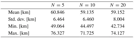
to the corresponding edge. There are many possibilities of connecting nodes, called the spanning tree, but a minimum spanning tree (MST) has the least sum of weights for all connecting edges among all spanning trees. Since most of the geodetic measurements today are predominantly GPS observations, the baseline length is a critical issue because the measurement error increases with increases in the base-line. Therefore, the MST can also be a possible means to evaluate the degree of network optimization. Figure 9 shows the MST of the optimally chosen network stations with DEM weighting (Fig. 7), computed using Prim’s al-gorithm (Cormenet al., 2001). By constraining the mean length from MST, we have selected 42 stations using the optimal method proposed in this study. To verify the op-timality of the approach, the statistics of the MST for dif-ferent number of candidate stations in the selection process are presented (Table 1). As can be seen in the table, the variation in the baseline length becomes significant as the number of candidate stations increases. The reason for this is that geometric optimality is encroached to some extent by the large number of candidate stations that are scattered. Indeed, it is difficult to determine an absolute standard for the number of candidates; one possibility is to use the top ten (10) candidate stations to select network stations in the optimization process.
Table 1. Statistics of the minimum spanning tree of the chosen network stations (N=Number of candidate stations).
N=5 N=10 N=20
Mean [km] 60.846 59.135 59.152
Std. dev. [km] 6.464 6.460 8.004
Min. [km] 49.064 44.497 42.734
Max. [km] 76.327 71.725 74.127
chain. Excluding these exceptions, the baseline length is fairly well distributed and shows a small variation around the mean value of 59 km. Therefore, the MST and mean and/or maximum baseline length can also be a criterion for completion of the network selection process.
8.
Discussion
The homogeneous and isotropic network design reported here was performed as a geometric approach to optimiza-tion. The topography, however, is also an important fac-tor when the aim is to provide a better explanation of the localized network in Korea, combined with the geometric solution. The Korean peninsula is topographically charac-terized by the presence of high mountain chains on the east coast and south-west area, and this is clearly indicated in the weight matrix (see Fig. 8). Thus, the topographic infor-mation was incorporated into the optimal network design for an optimization that is more appropriate to Korea.
Once the smoothed data are removed, the DEM residuals are used to determine the weights for each candidate station. The weight map based on DEM shows the variation along the E-W direction of Korea, and the chosen network stations follow the pattern of the mountain chain along the N-S direction that better conforms to Korea. The stations are more densely located on the east coast due to the rough terrain in that area.
The number of stations in the network is dependent on the budget, but the MST can be one of the alternative criteria to control the number of stations. Since the MST connects the entire network with a minimum cost (baseline length), it is possible to have the uniform baseline lengths throughout the network, resulting in high possibilities of stable solu-tion. Other approaches, such as nding a location using the least-squares solution instead of selecting a station from the candidates, need to be investigated further.
Acknowledgments. This research was supported by Basic Sci-ence Research Program through the National Research Foundation of Korea (NRF) funded by the Ministry of Education, Science and Technology (2009-0069542).
References
Bae, T.-S., Optimized network of ground stations for LEO orbit determi-nation,ION 2005 NTM, 515–522, 2005.
Cormen, T., C. Leiserson, R. Rivest, and C. Stein,Introduction to Algo-rithms (2nd), 1216 pp., McGraw-Hill, 2001.
Jekeli, C., Fourier Geodesy, The Ohio State University, Columbus, Ohio, 2007.
Grafarend, E.,Genauigkeitsmaße geod¨atischer Netze, Publ. DGK A-73, M¨unchen, 1972.
Grafarend, E. and B. Schaffrin, Kriterion-Matrizen I—zweidimensionale homogene und isotrope geod¨atische Netze,Z. Vermessungswesen,104, 133–149, 1979.
Kuang, S.,Geodetic Network Analysis and Optimal Design: Concepts and Applications, 368 pp., Sams Publications, 1996.
Schaffrin, B., Network design, inOptimization and Design of Geodetic Networks, edited by Grafarend, E. and F. Sans`o, 548–597, Springer-Verlag, 1985.
Schmitt, G., Second order design of free distance networks considering dif-ferent types of criterion matrices,Bull. Geodetica,54, 531–543, 1980. Wimmer, H.,Ein Beitrag zur Gewichtsoptimierung geod¨atischer Netze,
254 pp., Publ. DGK C-269, M¨unchen, 1982.