R E S E A R C H
Open Access
Threshold selection method for UWB TOA
estimation based on wavelet
decomposition and kurtosis analysis
Juan Li
1, Xuerong Cui
1*, Houbing Song
2, Zhongwei Li
1and Jianhang Liu
1Abstract
In wireless sensor networks, ranging or positioning via ultra-wideband (UWB) has caused widespread research interests where the non-coherent energy detection (ED) method with low sampling rate and low complexity is widely studied. However, the traditional energy detection methods only analyze the signal energy in the time domain, so their error is relatively large. In this paper, the simulation results show that most of the signal energy concentrates in the low-frequency band, so a novel threshold selection method for time of arrival (TOA) estimation is proposed that analyzes the signals in both time domain and frequency domain. In this method, the received signal is decomposed by
“db6”wavelet and the kurtosis of energy blocks of the low-frequency wavelet coefficients (Kc) is analyzed. At last, the mapping relationship betweenKcand the normalized threshold for TOA estimation is created using polynomial fitting with degree 3. The simulation results show that the TOA estimation error of the proposed method is significantly less than the method without wavelet decomposition.
Keywords:Ranging, Wavelet decomposition, Kurtosis analysis, Ultra-wideband, Energy detection, Threshold selection
1 Introduction
In recent years, with the development of wireless commu-nication technologies [1, 2], the applications of wireless sensor networks are more and more widely used. The im-portant premise of these applications is to obtain the pre-cise position of the targets [3–5]. Therefore, the precise positioning of targets becomes the key problem to be solved urgently.
Ultra-wideband (UWB) is a new wireless communica-tion technology [6–9], which is widely used in many fields, such as indoor short-distance communication, high-speed wireless local area networks (WLAN) [10], security monitoring, ranging, positioning, and so on. UWB is the most promising technology for indoor posi-tioning and tracking [3]. Compared with other short-range communication technology, UWB has many advantages for short-range communication: first, UWB can provide up to GHz bandwidth; second, UWB can provide data rates of hundreds of megabits per second
or even gigabits per second, so it is an ideal technology for wireless communication in wireless sensor networks [11, 12]; third, continuous transmission carrier is not needed in UWB communication, and the intermittent pulse is used to transmit data, which make short pulse duration, low power consumption, and high multipath resolution.
Wireless positioning methods can be divided into fin-gerprint positioning algorithm based on received signal strength indicator (RSSI) [13], geometric or range posi-tioning algorithm based on the range, time of arrival (TOA) [14, 15], time difference of arrival (TDOA) [16], or angle of arrival (AOA) [17], and some fusion posi-tioning methods together with inertial measurement units (IMUs) [5]. The signal fingerprint positioning algo-rithm [4, 18] is based on the mapping relationship between some parameters obtained from the received signal and the position information of the target node. The range-based positioning algorithm with round-trip-time (RTT) measurements [19] is often used to meet the requirement of high-precision positioning because of its high time delay resolution. However, obtaining the accurate ranging estimation is a very challenging * Correspondence:[email protected]
1Department of Computer and Communication Engineering, China University of Petroleum (East China), Qingdao 266580, China Full list of author information is available at the end of the article
problem due to the effects of thermal noise, multi-path fading, non-line of sight, and other factors in wireless transmission channel. For example, in non-line of sight (NLOS) environment, the range estimation based on TOA will typically be positively biased [3].
In recent years, ranging algorithms for UWB systems have been extensively studied. There are three main approaches. The first approach is matched filter (MF) based on coherent algorithm with high sampling rate [20]. The second is machine learning method based on some selected channel parameters. In [3], a ranging method based on kernel principal component is pro-posed, where the channel parameters are projected onto a high-dimensional nonlinear orthogonal space, and then the subset from these projections is used for ranging. The third is energy detection (ED) algorithm based on non-coherent receiver with low sampling rate and low complexity [8, 9, 21]. The matched filter approach is not applicable in many practical situations due to the high complexity and high hardware requirement. As opposed to the complex matched filter method, the energy detec-tion is a non-coherent method for TOA estimadetec-tion which consists of a square-law device, an integrator, a sampler, and a decision mechanism. The TOA value is estimated by the first signal sample exceeding a specific threshold which is deemed as the start of the received signal. Thus, the energy detection method is applicable in many cases because it is a method with low complex-ity and low sampling rate. In this method, how to select an appropriate threshold is a key issue. In literature [9], a threshold selection method based on kurtosis analysis of energy blocks was proposed, and in literature [21], a threshold selection method based on skewness analysis of energy blocks was also put forward. However, the TOA estimation accuracy of these methods is not very high because these parameters such as kurtosis of the re-ceived signals can only reflect statistical characteristics in time domain and ignore all the characteristics in fre-quency domain. At the same time, the received signals will be affected by the random noise, so the large ran-domness will result in the poor precision of kurtosis in time domain.
In this paper, the simulations of UWB signal spectrum under different signal to noise ratio (SNR) find out that the UWB signal energy is mainly distributed in the low-frequency band, while the energy of the white Gauss noise is evenly distributed over the entire frequency band. The wavelet transform is equivalent to two chan-nel filter banks with low-pass and high-pass characteris-tics, so using the wavelet transform, most of the signal energy concentrates in the low-frequency coefficients, while the energy of white Gauss noise distributes in the coefficients of all frequency bands. Thus, in this paper, after the wavelet transform used in the received signal,
the high-frequency coefficients are discarded, and only the low-frequency coefficients are used as the received signal energy to improve the accuracy of ranging. In this way, the white Gauss noise interference in the signal can be reduced effectively.
The remainder of this paper is organized as follows. In Section 2, the UWB ranging system model is presented. Section 3 discusses some ranging estimation algorithms based on traditional energy detection method in the time domain. Section 4 introduces the proposed thresh-old selection method for TOA estimation based on wavelet decomposition, energy detection, and kurtosis analysis. In Section 5, the simulation results and the per-formance discussion are presented, and Section 6 con-cludes the paper.
2 UWB ranging system models 2.1 Pulse waveform
In UWB ranging system, short pulses with sharp rising and falling edges are usually used as the transmitting sig-nal to get shorter pulse duration (nanosecond level) or higher time delay resolution.
The second derivative of Gauss function is in accord with this characteristic, so it is used as the UWB pulse signal, which can be expressed as Eq. (1)
f tð Þ ¼d
where q(t) is the Gaussian pulse, α denotes the shape factor of the waveform, and a smaller value ofα results in a shorter pulse.
2.2 Modulation method
In order to improve the capacity of anti-interference, pulse position modulation (PPM) and time hopping spread spectrum (TH-SS) [7] are used which can be expressed as Eq. (2)
s tð Þ ¼X
i
f t−iTf−ciTc−aiε
ð2Þ
where frame index and frame duration are denoted by i
and Tfrespectively,Tc is the chip duration, hopping
se-quence is composed of integer-valued ci∈{0, 1,…,Tf/Tc
−1}, ai is a binary sequence, andε is the time shift in
pulse position modulation.
2.3 IEEE 802.15.4a channel model
impulse radio ultra-wideband (IR-UWB) and chirp spread spectrum (CSS). The former is used for ranging, and the latter is used for wireless communication. Since this paper is focused on TOA estimation or ranging algorithm, therefore, only the IR-UWB is considered in line of sight (LOS) and NLOS environments. Classifica-tion of channel models in IEEE 802.15.4a are listed in in Table 1.
CM1 and CM2 are the indoor residential channel models with LOS and NLOS environments which are used for the simulations in this paper. The channel im-pulse response can be expressed as Eq. (3)
h tð Þ ¼X
whereLis the number of received clusters,K(l) denotes the number of received multipath components in thelth cluster,αl, kis the gain factor of thekth multipath
com-ponent of the lth cluster,Tldenotes the TOA of the lth
cluster, andτl,kis the TOA of thekth multipath
compo-nent of the lth cluster. The environments of CM1 and CM2 are shown in Table2.
The received signal can be expressed as Eq. (4)
r tð Þ ¼s tð Þ h tð Þ þn tð Þ ð4Þ where n(t) is the additive white Gaussian noise (AWGN) with zero mean and two-sided power spec-tral density N0/2. Thus, the received signal can be
expressed as Eq. (5)
2.4 TOA estimation error
The mean absolute error (MAE) of TOA estimation re-sults is expressed as Eq. (6)
MAE¼ 1
N
XN
n¼1
∣tn−^tn∣ ð6Þ
where tn is the real TOA, tn denotes the estimated
TOA, andNis the simulation times.
3 Energy detection method
As shown in Fig. 1, in the traditional energy detection methods, the received signal is squared by the low noise amplifier, and then input into an integrator with period Tb which is much longer than the sampling interval, so the number of energy blocks within a frame isNb=⌊Tf/ Tb⌋ (⌊⌋denotes the integer part) and Tf is the frame period.
Thus, the sample values of integrator output are given by Eq. (7)
in each integration period, and Np is the pulse number
in one symbol. In this paper,Np= 1, so the sample values
of integrator output are given by Eq. (8)
z n½ ¼
There are many TOA estimation methods based on the energy blocksz[n] which can detect the start of a re-ceived signal or estimate the TOA. The simplest one is the maximum energy method, which chooses the max-imum energy block z[n] as the first received signal and Table 1Classification of channel models specified in IEEE
802.15.4a standard
Channel models
Channel description
CM1 Residential environment with LOS communication (7–20 m)
CM2 Residential environment with NLOS communication (7–20 m)
CM3 Office environment with LOS communication (3–28 m)
CM4 Office environment with NLOS communication (3–28 m)
CM5 Outdoor environment with LOS communication (5–17 m)
CM6 Outdoor environment with NLOS communication (5–17 m)
CM7 Industrial environment with LOS communication (2–8 m)
CM8 Industrial environment with NLOS communication (2–8 m)
CM9 Open outdoor environment with NLOS communication (e.g., farm, snow-covered area)
Table 2Channel parameters of CM1 and CM2
Channel parameters CM1
(LOS)
CM2 (NLOS)
Frequency dependency of the channel 1.12 1.53
Standard deviation of the log-normal shadowing of entire impulse response
2.22 3.51
Mean number of clusters 3 3.5
Cluster arrival rate 0.047 0.12
Two ray arrival rates (rays per nanosecond) for mixture of Poisson processes
1.54, 0.15 1.77, 0.15
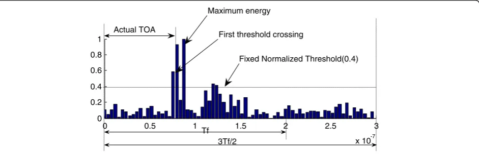
the TOA is equal to time responding to the center of the block. However, as shown in Fig. 2, usually, the max-imum z[n] is not responding to the first received signal; in this case, the estimated TOA will have big error, espe-cially in NLOS environments. Thus, threshold crossing method has been proposed; with this method, the received energy blocksz[n] are compared with a selected threshold. In this case, the TOA estimation can be ob-tained according to the first threshold exceeding sample index, which is expressed as Eq. (9)
^tTC¼½minfnjz n½ >ξg−0:5Tb; ð9Þ
It is very difficult to determine an appropriate thresh-old ξ directly because if the big change of energy and signal, so a normalized threshold ξnorm ranging from 0
to 1 is often used which is expressed as Eq. (10)
ξnorm¼ ξ−
minfz n½ g
maxfz n½ g−minfz n½ g: ð10Þ
In [9], the kurtosis of received energy blocks z[n] is employed to choose the appropriate normalized thresh-old. Kurtosis can be expressed as Eq. (11),
k¼ 1
where z and δ denote the mean and standard deviation of z[n] respectively. In this case, the ranging estimation can be expressed as Eq. (12)
D¼C ^tTC; ð12Þ
whereC is the speed of electromagnetic wave in the air andtTC denotes the TOA estimate of signal.
In a positioning system, the coordinates of the target nodes (x,y,z) at the intersection of the circles of the ref-erence nodes can be obtained by solving the following equations
node, and Dk is the range from the target node to the
kth reference node.
4 The proposed threshold selection method 4.1 Low-frequency wavelet coefficient
Wavelet transform has the characteristics of multi-resolution analysis, and the received signal is divided into low-frequency part and high-frequency part using the wavelet decomposition. In the next layer process of wavelet decomposition, the low-frequency part is further divided into low-frequency part and high-frequency part, but the high-frequency part is no longer decomposed. Fig. 1Block diagram of the energy detection method
0 0.5 1 1.5 2 2.5 3
Figure 3 shows a three-level wavelet decomposition tree. Multi-resolution analysis is used to decompose the low-frequency part of the signal to improve the reso-lution of the frequency. For the signal S, it is decom-posed into high-frequency part D1 and low-frequency partA1, and then the low-frequency part ofA1 is further decomposed into high-frequency part D2 and low-frequency part A2. And so on, the approximation part and detail part at any scales (resolutions) can be decomposed.
The above process of wavelet decomposition can be expressed as Eq. (14)
cjþ1ð Þ ¼k
P
n h nð −2kÞcjð Þn
djþ1ð Þ ¼k
P
n g nð −2kÞcjð Þ;n 8
<
: ð14Þ
where c0 is the received UWB signal, j∈{0, 1, 2,…}
de-notes the levels of decomposition, cj is the
low-frequency coefficient using the j-level wavelet decom-position, and dj is the high-frequency coefficient using
thej-level wavelet decomposition.h(n) represents a low-pass filter, and g(n) represents a high-pass filter, which are determined by the type of the selected wavelet.
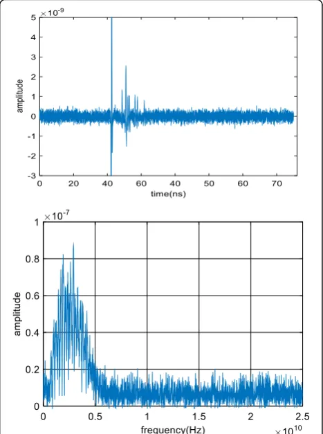
In order to analyze the time domain waveform and en-ergy spectrum of UWB, different values of Eb/ N0={40 dB, 35 dB, 30 dB} are simulated, whereEbis the energy in each bit and N0 is one-sided power spectral
density of additive white Gaussian noise. The parameters of the UWB transmission system are set as: Tf= 50 ns, Tc= 1 ns , ε= 0.5 ns, sampling frequency Fc= 50 GHz, and transmission delay = 20 ns. The simulation results are shown in Figs. 4, 5, and 6.
From the above simulations, the following conclusions can be drawn:
(1)Either in time domain or in frequency domain, when SNR decreases, the amplitude of the noise increases obviously comparing with the amplitude of the signal.
(2)The energy of signal is mainly distributed in the low frequency band, while the energy of white Gauss
noise is evenly distributed over the entire frequency band.
Because the wavelet decomposition is equivalent to two channel filter banks with low-pass and high-pass characteristics, after the wavelet decomposition, most energy of the received UWB signal concentrates in the coefficients of low-frequency bands, while the energy of the white Gauss noise distributes in the coefficients of different frequency bands. Therefore, in the energy de-tection receiver of this paper, after the wavelet trans-form, the high-frequency wavelet coefficients are discarded, and only the low-frequency wavelet coeffi-cient is regarded as the received energy to improve the accuracy of ranging. In this way, the white Gauss noise interference in the signal can be reduced effectively.
4.2 Kurtosis of the energy blocks of low-frequency coefficients
In order to examine the characteristics of kurtosis of the energy blocks of the received signal (Ks) [9] and the
kur-tosis of the energy blocks of the decomposed low-frequency wavelet coefficients (Kc), the CM1 (residential
LOS) and CM2 (residential NLOS) channel models in Fig. 3Three-level wavelet decomposition
the IEEE802.15.4a standard are employed. Ks can be
expressed as Eq. (15),
Ks¼
1
Ns−1 ð Þδ4
XNs
n¼1
Zs½ −n Zs
4
−3; ð15Þ
whereZs[n] is the received signal energy blocks, Zs and δ denote the mean and standard deviation of Zs[n]
re-spectively. The number of samples in each energy inte-gration interval is represented asNi=Tb×Fc, where Tb
is the integration period, and Fc is the sampling
fre-quency. The number of signal samples in each frame is represented as Nf=Tf × Fc, where Tf is the frame
period. The number of energy blocks within a frame is Ns¼
b
NNfic
¼Nb, where ⌊⌋ denotes the integer part.Kccan be expressed as Eq. (16),
Kc¼
1
Nc−1 ð Þδ4
XNc
n¼1
Zc½ nZc
4
−3; ð16Þ
where Zc[n] is the energy blocks of the decomposed
low-frequency coefficients, Z and δ denote the mean
and standard deviation of Zc[n] respectively. The
num-ber of the low-frequency coefficients in each integration intervalNicis represented as Eq. (17)
Nic¼
⌊
TbFcNfc
Nf
⌋
;ð17Þ
where Nfc is the number of the low-frequency
coeffi-cients in each frame. And then the number of the energy blocks of low-frequency coefficients is Eq. (18)
Nc¼
⌊
Nfc
Nic
⌋
:ð18Þ
For each Eb/N0 value of {5 dB, 6 dB, ..., 25 dB}, 1000
channel realizations were generated with Fc= 50 GHz.
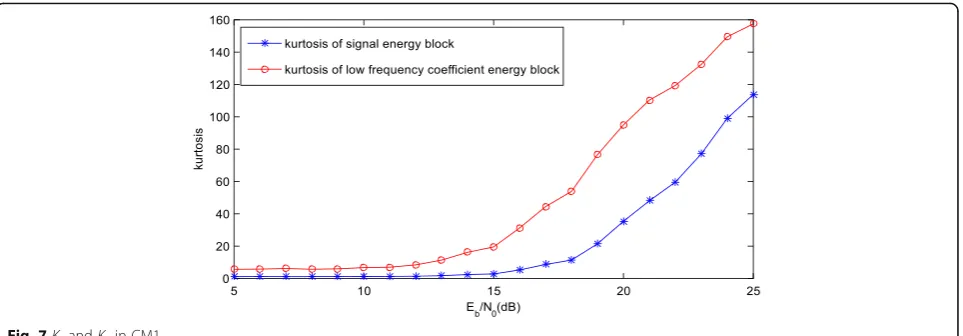
The second derivative Gaussian pulse was employed withTb= 0.2 ns,Tf= 50 ns, andNs= 1. The“db6” wave-let with two-layer decomposition was used. The simula-tion of averageKsandKcare as shown in Figs. 7 and 8.
Figures 7 and 8 illustrate that the characteristics ofKs
andKcwith respect to different values ofEb/N0is almost
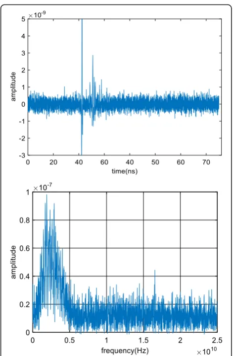
Fig. 5Time domain waveform and energy spectrum withEb/N0=35 dB
the same for the two different channels. Furthermore, Figs. 7 and 8 show that Ks andKc increase as Eb/N0
in-creases, butKcchanges more rapidly. Therefore,Kccan
better reflect the changes with different values ofEb/N0
and it is more suitable for threshold selection.
4.3 Relationship between Kcand threshold
To determine the optimal threshold ξbest based on Kc,
the relationship between the MAE,Kc, and the
normal-ized threshold ξnorm for different Kc was determined.
One thousand channel realizations with different values of Eb/N0were simulated. There are four steps to
estab-lish the relationship:
(1)Generate a large amount of receive signals for each channel model under differentEb/N0values of {5 dB, 6 dB,…, 25 dB}.
(2)Calculate the average MAE values with respect to different normalized thresholdsξnormof {0.1, 0.2,…,
1.0} for eachKcvalue. With each channel realization, the thresholds are compared withZc[n] to find the first sample index crossing the normalized threshold, as shown in Eq. (10). In the simulation, because of the random noise signal, there are different MAE values with respect to one specific normalized threshold and one specificEb/N0value, so the average MAE is calculated with respect to one specific normalized threshold. Moreover, becauseKcis a real value,Kcis rounded to the nearest integer value.
(3)Select the normalized threshold with the lowest MAE as the best thresholdξbestwith respect to specific Kc for each channel model.
(4)A polynomial with degree 3 is fitted to the best threshold ξbest for each value ofKc by using the method of least-squares where Kc is the x -coord-inate and ξbest is they-coordinate. To obtain the coefficient estimates, the least-squares method minimizes the summed square of residuals. The
Fig. 7KsandKcin CM1
ith residualri for the ith pair of (Kc, ξbest) is defined as
ri¼yi−^yi; ð19Þ
whereyiis the best threshold andŷiis the fitted
thresh-old value for theithKc, so the summed square of
resid-ualsSKis given by
SK ¼ Xn
i¼1
r2i ¼X
n
i¼1
yi−^yi
ð Þ2 ð
20Þ
where n is the number of (Kc, ξbest). The fitting result
based onKcare shown in Eq. (21)
CM1:ξc1¼ −3:107910−8Kc3þ2:519110−5Kc2−7:046210−3 Kcþ0:82585
CM2:ξc1¼−2:698810−8Kc3þ2:268110−5Kc2−6:521410−3 Kcþ0:7816:
ð21Þ
where ξc1 and ξc1 are the optimal thresholds for CM1
and CM2.
5 Performance results and discussion 5.1 TOA estimation error
In order to compare with the method without wavelet decomposition [9], the optimal thresholdsξs1andξs1for
CM1 channel and CM2 channel based onKs are
gener-ated as Eq. (22) using the similar method as shown in [9].
CM1:ξs1 ¼−8:051410−8Ks3þ4:523210−5Ks2−8:754610−3 Ksþ0:78051
CM2: ξs1 ¼−7:729110−8Ks3þ4:437410−5Ks2−8:724610−3 Ksþ0:76794
ð22Þ
In this section, the MAE is examined forKc-based and
Ks-based threshold selection algorithms in the CM1 and
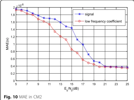
CM2 channel models of IEEE 802.15.4a standards. As before, 1000 channel realizations were simulated for each case. The performance results are shown in Figs. 9 and 10.
Figures 9 and 10 present the following:
(1)In CM1 and CM2, the MAE of theKc-based andK s-based threshold selection methods decrease as the Eb/N0increase. But whenEb/N0is between 9 and 20 dB, the proposed method is better than that of
theKs-based method proposed in [9]. It can be
found that in CM1 channel, whenEb/N0is 14 dB, the MAE ofKc-based method is about 5 ns better than that of theKs-based method. In CM2 channel, whenEb/N0is 15 dB, MAE ofKc-based method is
about 5.87 ns better than that of theKs-based method.
(2)WhenEb/N0is less than 8 dB, the MAE of the two algorithms are very near. This is because now the energy of the noise is very high, which will affect the decomposed low-frequency coefficients seriously, so the advantage of the proposed method is little compared with theKs-based method.
(3)WhenEb/N0is higher than 21 dB, the MAE of the two methods is almost the same. This is because now the energy of the noise is very low compared with the signal energy, which will not affect the two methods.
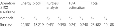
5.2 Computational complexity
In order to compare the computational complexity of different methods, 100 iterations were performed for eachEb/N0value of {5 dB, 6 dB, ..., 25 dB}, and the total
running time of 100 × 25 = 2100 iterations is given in Table 3. In the simulation, the amount of energy blocks of Kc is 472 and for Ks is 375. At the same time, the
Fig. 9MAE in CM1
signal decomposed using wavelet transform needs extra computation, so the running time of the Kcmethod is a
little higher than that of the Ks method. For Each TOA
estimation process, the difference of running time is just 2 ms, so this is acceptable.
6 Conclusions
In the UWB ranging system, the energy detection method based on non-coherent receiver is widely used. However, because of the interference, such as multi-path fading, thermal noise, inter-symbol interference, and reflection interference, the precision of ranging is not very high. The simulation results show that in the UWB signal decom-posed by wavelet transform, most of the signal energy is concentrated in the low-frequency band, while the energy of noise is evenly distributed over the entire frequency band. Therefore, this paper proposes a new threshold selection method based on wavelet decomposition and kurtosis analysis, that is, the UWB signal is decomposed by wavelet transform, the threshold is obtained based on the kurtosis of energy blocks of low-frequency wavelet coefficient, and then the first energy block exceeding the threshold is treated as the TOA of signal. The simulation results show that the new method can obviously improve the precision of TOA estimation.
Acknowledgements
This work was supported by the National Natural Science Foundation of China under Grant No. 61671482, the Nature Science Foundation of Shandong Province No. ZR2014FL014, and the Fundamental Research Funds for the Central Universities Nos. 16CX02046A, 17CX02042A, and 14CX02212A.
Authors’contributions
The authors have contributed jointly to all parts on the preparation of this manuscript, and all authors read and approved the final manuscript.
Competing interests
The authors declare that they have no competing interests.
Publisher’s Note
Springer Nature remains neutral with regard to jurisdictional claims in published maps and institutional affiliations.
Author details 1
Department of Computer and Communication Engineering, China University of Petroleum (East China), Qingdao 266580, China.2Department of Electrical, Computer, Software, and Systems Engineering, Embry-Riddle Aeronautical University, Daytona Beach, FL 32114, USA.
Received: 27 August 2017 Accepted: 15 November 2017
References
1. X Zheng, Z Cai, J Li, H Gao, A study on application-aware scheduling in wireless networks. IEEE Trans. Mob. Comput.16(7), 1787–1801 (2017). https://doi.org/10.1109/TMC.2016.2613529
2. S Cheng, Z Cai, J Li, Curve query processing in wireless sensor networks. IEEE Trans. Veh. Technol.64(11), 5198–5209 (2015). https://doi.org/10.1109/ TVT.2014.2375330
3. V Savic, EG Larsson, J Ferrer-Coll, P Stenumgaard, Kernel methods for accurate UWB-based ranging with reduced complexity. IEEE Trans. Wirel. Commun.15(3), 1783–1793 (2016). https://doi.org/10.1109/TWC.2015. 2496584
4. F Simone, R Francescantonio Della, inmobile positioning and tracking: from conventional to cooperative techniques. Fundamentals of positioning (Wiley-IEEE Press, New Jersey, United States, 2017), p. 416
5. PK Yoon, S Zihajehzadeh, BS Kang, EJ Park, Robust biomechanical model-based 3-D indoor localization and tracking method using UWB and IMU. IEEE Sensors J.17(4), 1084–1096 (2017). https://doi.org/10.1109/JSEN.2016. 2639530
6. Z He, Z Cai, S Cheng, X Wang, Approximate aggregation for tracking quantiles and range countings in wireless sensor networks. Theor. Comput. Sci.607, 381–390 (2015). https://doi.org/10.1016/j.tcs.2015.07.056 7. MZ Win, RA Scholtz, Ultra-wide bandwidth time-hopping spread-spectrum
impulse radio for wireless multiple-access communications. IEEE Trans. Commun.48(4), 679–689 (2000). https://doi.org/10.1109/26.843135 8. I Guvenc, Z Sahinoglu, inICU 2005: 2005 IEEE International Conference on
Ultra-Wideband. Threshold-based TOA estimation for impulse radio UWB systems (Switzerland, Zurich, 2005), pp. 420–425. https://doi.org/10.1109/ ICU.2005.1570024
9. I Guvenc, Z Sahinoglu, Threshold selection for UWB TOA estimation based on kurtosis analysis. IEEE Commun. Lett.9(12), 1025–1027 (2005). https://doi. org/10.1109/LCOMM.2005.1576576
10. S Cheng, Z Cai, J Li, X Fang, in2015 IEEE Conference on Computer Communications (INFOCOM). Drawing dominant dataset from big sensory data in wireless sensor networks (2015), pp. 531–539. https://doi.org/10. 1109/INFOCOM.2015.7218420
11. J Li, S Cheng, Y Li, Z Cai, in2015 IEEE 35th International Conference on Distributed Computing Systems. Approximate holistic aggregation in wireless sensor networks (2015), pp. 740–741. https://doi.org/10.1109/ICDCS.2015.86 12. S Cheng, Z Cai, J Li, H Gao, Extracting kernel dataset from big sensory data
in wireless sensor networks. IEEE Trans. Knowl. Data Eng.29(4), 813–827 (2017). https://doi.org/10.1109/TKDE.2016.2645212
13. Z Xiao, H Wen, A Markham, N Trigoni, P Blunsom, J Frolik, Non-line-of-sight identification and mitigation using received signal strength. IEEE Trans. Wirel. Commun.14(3), 1689–1702 (2015). https://doi.org/10.1109/TWC.2014.2372341 14. E Arias-de-Reyna, JJ Murillo-Fuentes, R Boloix-Tortosa, Blind low complexity time-of-arrival estimation algorithm for UWB signals. IEEE Signal Processing Letters22(11), 2019–2023 (2015). https://doi.org/10.1109/LSP.2015.2450999 15. V Savic, J Ferrer-Coll, P Ängskog, J Chilo, P Stenumgaard, EG Larsson,
Measurement analysis and channel modeling for TOA-based ranging in tunnels. IEEE Trans. Wirel. Commun.14(1), 456–467 (2015). https://doi.org/ 10.1109/TWC.2014.2350493
16. A Jafari, T Mavridis, L Petrillo, J Sarrazin, M Peter, W Keusgen, PD Doncker, A Benlarbi-Delai, UWB Interferometry TDOA estimation for 60-GHz OFDM communication systems. IEEE Antennas and Wireless Propagation Letters 15, 1438–1441 (2016). https://doi.org/10.1109/LAWP.2015.2512327 17. BG Yu, G Lee, HG Han, WS Ra, TW Kim, A time-based angle-of-arrival sensor
using CMOS IR-UWB transceivers. IEEE Sensors J.16(14), 5563–5571 (2016). https://doi.org/10.1109/JSEN.2016.2567441
18. S Büyükçorak, T Erbaş, GK Kurt, A Yongaçoğlu, in2014 22nd Signal Processing and Communications Applications Conference (SIU). Indoor localization applications (2014), pp. 1239–1242. https://doi.org/10.1109/SIU.2014.6830460 19. GD Angelis, A Moschitta, P Carbone, Positioning techniques in indoor
environments based on stochastic modeling of UWB round-trip-time measurements. IEEE Trans. Intell. Transp. Syst.17(8), 2272–2281 (2016). https://doi.org/10.1109/TITS.2016.2516822
20. AYZ Xu, A E K S, W A K S, W Qin, A novel threshold-based coherent TOA estimation for IR-UWB systems. IEEE Trans. Veh. Technol.58(8), 4675–4681 (2009). https://doi.org/10.1109/TVT.2009.2020990
Table 3Running time of different methods
Operation
21. X Cui, H Zhang, TA Gulliver, Threshold selection for ultra-wideband TOA estimation based on neural networks. Journal of Networks7(9), 1311–1318 (2012). https://doi.org/10.4304/jnw.7.9.1311-1318