R E S E A R C H
Open Access
Location estimation using RSS measurements
with unknown path loss exponents
Musa Bora Zeytinci, Veli Sari, Frederic Kerem Harmanciˆ, Emin Anarim and Mehmet Akar
*Abstract
The location of a mobile station (MS) in a cellular network can be estimated using received signal strength (RSS) measurements that are available from control channels of nearby base stations. Most of the recent RSS-based location estimation methods that are available in the literature rely on the rather unrealistic assumption that signal
propagation characteristics are known and independent of time variations and the environment. In this paper, we propose an RSS-based location estimation technique, so-called multiple path loss exponent algorithm (RSS-MPLE), which jointly estimates the propagation parameters and the MS position. The RSS-MPLE method incorporates antenna radiation pattern information into the signal model and determines the maximum likelihood estimate of unknown parameters by employing the Levenberg-Marquardt method. The accuracy of the proposed method is further examined by deriving the Cramer-Rao bound. The performance of the RSS-MPLE algorithm is evaluated for various scenarios via simulation results which confirm that the proposed scheme provides a practical position estimator that is not only accurate but also robust against the variations in the signal propagation characteristics. Keywords: Mobile positioning; Location estimation; Cramer-Rao bound; Received signal strength
1 Introduction
Recently, location estimation has been among the most attractive research topics in the area of cellular commu-nications. With accurate position estimation, a variety of applications and services such as emergency services, monitoring and tracking fraud protection, asset tracking, fleet management, mobile yellow pages, and even cellular system design and management can become feasible for cellular networks [1]. These potential applications of wire-less positioning have also been recognized by the IEEE, which set up a standardization group 802.15.4a for design-ing a new physical layer for low-data rate communications combined with positioning capabilities [2]. Furthermore, the Federal Communications Commission (FCC) in the USA has required wireless providers to locate mobile users within tens of meters for emergency 911 calls [3].
The position of a mobile station (MS) can be determined using multiple radio signals transmitted or received by the MS. Some location estimation methods like assisted
*Correspondence: [email protected] ˆDeceased
Department of Electrical and Electronics Engineering, Bogazici University, Bebek, Istanbul, Turkey
global positioning system (A-GPS) are based on signals transmitted from satellites, while others rely on mea-surements of signals between MS and base stations (BS), the so-called network-based methods. Currently, the best positioning accuracy in cellular systems is provided by A-GPS at the expense of a significant increase in network and handset complexity [4]. For instance, modifications on the handset such as an embedded GPS receiver and deployment of location management units (LMU) into the network are needed in order to operate A-GPS systems [5]. Compared to A-GPS, network-based methods are rel-atively less complex. Moreover, they can be used in many situations where the A-GPS method cannot be applied, i.e., indoor positioning, but generally with a degradation in accuracy. So far, a wide variety of network-based posi-tioning techniques have been proposed which use mea-surements obtained within the cellular networks, such as received signal strength (RSS), time of arrival (TOA), time difference of arrival (TDOA), and angle of arrival (AOA) methods [6-15].
Positioning technology is often based on trilateration in time-based methods like TOA and TDOA, in which the MS position is obtained as the intersection point of
three circles constituted by distance estimates [16]. Assur-ance of proper operation of time-based methods requires the deployment of LMUs [17]. These network elements perform timing measurements of all local transmitters, based on which the actual relative time difference for each BS can be estimated. In a similar manner, AOA-based positioning methods require the implementation of adaptive array antennas, by which the direction of signal arrival can be estimated. At the same time, the handset typically requires software modifications to enable posi-tioning functionality with such a method. Consequently, these methods are not widespread in commercial systems due to their high deployment costs. Therefore, improving the accuracy of positioning systems based on the exist-ing cellular network infrastructure is desired, which is the main motivation of this study.
The system model that is used for location estimation in this paper is based on RSS measurements. One funda-mental MS function is to find the BSs with the strongest signal strength for cell selection purposes. Thus, RSS-based methods can be implemented without any hard-ware enhancement in either the MS or the BS. Distance information between MS and BS can be extracted from RSS measurements using accurate information about the propagation characteristics of the measurement chan-nel. However, in most of the RSS-based location esti-mation techniques in the literature, it is assumed that the propagation parameters of the measurement channel are accurately known a priori, either through a train-ing period or by assumtrain-ing a perfect free-space channel condition [18-24]. Such an approach results in degraded positioning accuracy in many practical application scenar-ios, including mobile tracking techniques in [25,26]. More specifically, both [25,26] study Monte Carlo-based mobil-ity tracking algorithms under the assumption that the mobile moves in a 2D environment with input as accelera-tion. In [25], RSS data are used to predict mobile position and velocity using particle filtering techniques, but the method relies on known propagation parameters. In [26], the so-called interacting multiple model method has been extended to predict the state of the mobile for indoor applications by considering multiple fixed environment parameters at the expense of an increase in the number of random processes, whereas the technique herein relies on continuous parameter adaptation.
In this paper, a method that aims to resolve major short-comings of the existing RSS-based positioning techniques is proposed. In particular, an RSS-based location esti-mation technique that jointly estimates the propagation parameters and the MS position is explained in Section 2. The Cramer-Rao bound (CRB) derivation and accuracy evaluation are given in Section 3 as a benchmark for per-formance comparison. In Section 4, simulation results under various scenarios are presented to evaluate the
performance of the proposed algorithm. Finally, some concluding remarks are given in Section 5.
2 RSS-based location estimation model
Using RSS together with a path loss (PL) and shadow fad-ing model, a distance estimate between the BS and the MS can be obtained. The propagation model used through-out this paper is a modified version of the log normal model that is widely used in the literature [27-30]. The PL exponent (PLE) is the key parameter in the log normal model. An accurate value of the PLE is required in order to obtain an accurate estimate of the MS-BS distance from the corresponding RSS measurement.
In most of the existing studies of RSS-based location estimation techniques in the literature, the channel model is assumed to be known a priori, that is, the path loss characteristics of the coverage area are considered known, either by assuming that the environment is a perfect free space or by extensive measurement and modeling prior to the deployment of location estimation systems. However, the PLE parameter is environment dependent [31,32]. Even in the same environment, propagation characteris-tics may change considerably over a long period of time, e.g., due to seasonal and/or weather changes [33]. In [32], it is experimentally demonstrated in an omnidirectional antenna system that the PLE is strongly dependent on the base antenna height and theterrain category. Extension of the experimental study in [32] to directional antenna systems can be found in [34] where the authors show that antenna beamwidth has an additional gain reduc-tion influence on the PLE. In other experimental studies that consider path loss modeling for directional antenna systems [35,36], the authors compute different PLEs for differentareas of the cell that consist of different terrains (but not different PLEs for different directional anten-nas of the same base station). There are also related studies that utilize single PLE for directional antenna systems [37-39].
2.1 Antenna model
Point to multipoint and cellular communication systems commonly use fan-beam antennas for sector coverage. An approximate formula describing the normalized azimuth radiation pattern of the fan-beam antenna using three parameters is given by:
A(φ)=exp
−a3dB( | φ| φHBW
)τ
, (1)
wherea3dBis a unitless parameter that determines the pat-tern value at half power bandwidth (HBW)|φ| = φHBW (in radians) [40], i.e.,
a3dB= −ln( 1 √
2)=0.3465 (2)
andτ is used to match the pattern to a second field value, ν, at|φ| = |φν|where 0< ν <1, i.e.,
τ = ln(
−ln(ν) a3dB ) ln(|φν|
φ3dB)
(3)
In this paper, τ is evaluated at |φν| = π/2, and the
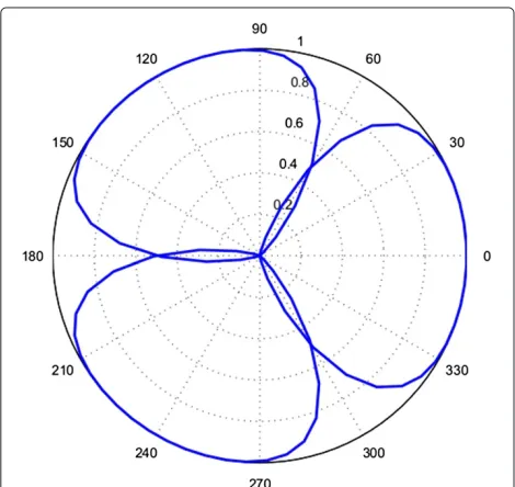
value ofνis taken to be equal to 0.006 that is the inverse of the front-to-side ratio of the normalized pattern and φHBW=π/3 is the recommended value according to ETSI EN 301 215-2 Class CS 2 requirement in a local multipoint distribution service point-to-multipoint application [40] (see Figure 1 for the radiation pattern used in this paper).
Figure 1Normalized radiation pattern for 3-sector BS configuration.
2.2 Path loss model
In cellular networks, an MS measures received signal code power on a common pilot channel (CPICH) in Univer-sal Mobile Telecommunications System (UMTS) and RSS on a broadcast control channel (BCCH) in GSM systems to determine the received signal level. Signal strength measurements are indexed with base station and sectoral identifiers k and s, respectively, in (4) [18] considering that transmitting cells use different channels (CPICHs or BCCHs):
Rk,s(x,y,αk)=
PGA2k,s(x,y)
β d
k,s(x,y) d0
αk10
−vk,s/10. (4)
In (4),Rk,sis the received signal strength from sectorsof base stationkat point(x,y)(in watts);Pis the total trans-mitted power on each sectors(in watts), andAk,s(x,y)and Gare the normalized radiation pattern and the antenna gain in azimuth direction, respectively, that belongs to the corresponding cell of sector s; d0 (in meters) is the free-space reference distance;d(x,y)(in meters) is the dis-tance between MS and BS at point (x,y); vk,s accounts for shadow fading;αk is the PLE that is specific forkth base station; andAk,s(φ)is represented asAk,s(x,y)since it is possible to determineφ with the knowledge of MS and BS coordinates. Herein, it is assumed thatP,G, and β are assumed to be knowna prioriandβ is calculated by [32]:
β =
4πd0 λ
2
, (5)
whereλis the wavelength in meters andd0is chosen to be equal to 1 m in a microcell environment [31]. Rewriting the RSS in decibel (dB), we have:
μk,s(dB)(θ )=10 log10
PG β
+20 log10Ak,s(x,y)
−10αklog10
dk,s(x,y) d0
Rk,s(dB)(θ )=μk,s(dB)(θ )−vk,s (6)
whereθ =x yα1 . . . αk T.
2.3 Problem formulation and the positioning algorithm Based on the path loss model described above, the distri-bution ofRk,s(dB)(θ )is Gaussian, i.e., we have:
denotes the pdf for the determin-istic unknown parameterθ[41]. AssumingRk,s(dB)is
inde-pendent and identically distributed (i.i.d.), the likelihood function,L(θ )can be written as:
where n is the number of BSs that have RSS measure-ments for the MS andmis the number of sectors for each BS. Taking into account thatRk,s(dB)is an i.i.d. Gaussian
random variable,L(θ )becomes:
L(θ )= 1
In order to obtain the maximum likelihood (ML) esti-mate,θMLthat best approximates the available data,L(θ ) should be maximized overθ (see [41], pp. 177). This in turn can be done by computing:
θML:=arg min
where arg min is the value ofθ for which the given func-tion is minimized over the given data set. Note that a distinctive advantage of ML estimate is that it can always be found for a given data set [41].
In this paper, we obtain this estimate using a recur-sive solution of a nonlinear least squares problem. To this end, defineJ(θ )to be the cost function (which is to be minimized so thatL(θ )in (9) is minimized):
J(θ )= sented in vector form as:
J(θ )=(R−μ(θ ))T(R−μ(θ ))=f(θ )Tf(θ ) (13)
Thus, any θ∗ that satisfies (14) is a solution of (10) if
f(θ∗)is nonsingular, i.e.,
0=Jθ∗=2fθ∗Tfθ∗ (14) In this paper, the Levenberg-Marquardt (LM) method which is a modified version of the Gauss-Newton method is employed to solve the nonlinear least squares problem [42,43]. The proposed algorithm which is summarized as Algorithm 1 on the next page employs a linear approxi-mation of the nonlinear equations to find a least squares estimate of these equations iteratively. The vector μ(θ ) that consists of nonlinear functions is linearized using the Taylor series expansion in which the second-order terms are omitted:
First-order Taylor series expansion is obtained for μk,s(dB)(θ )whereθ(0)is the initial estimate forθMLandJ(0) is the Jacobian matrix ofμk,s(dB)(θ )atθ(0). Consequently,
the LM step sizeat each iteration is obtained by solving:
JTJ+hI=JTf, (16) whereh>0, e.g., forn=2 BSs andm=3 sectors for each BS, in caseθ =x,y,α1,α2 are unknown parameters, the Jacobian matrixJcan be represented as:
J= dk represents the distance betweenkth BS and the MS, that is, dk(θ ) =
(x−xk)2+(y−yk)2. Herein,kindex represents the BS, andsrepresents the sector that belongs to BSk. Since each channel used by different BSs may have a distinct PLE,αparameters are indexed with BS ID,k.
Algorithm 1LM-based algorithm for joint estimation of propagation parameters and mobile position 1: (Initialization)
(i) Letd1be the initial radial distance estimate obtained using Cell ID + Timing advance (Cell ID + Round trip time in UMTS case). (Both of these measurements are available from the serving cell.)
(ii) Let the number of RSS measurements from different sectors of the same BS bens. Ifns=1, then letφbe the azimuth angle of the serving sector
else ifns>1, utilize the LM method (as in step 3 below) withθ =[φ,α1]andJ(θ )as follows:
J(θ )= ⎡ ⎢ ⎢ ⎣
∂(20 log(A11(φ)))
∂φ
−10α1log(d1)
∂α1
∂(20 log(A12(φ)))
∂φ
−10α1log(d1)
∂α1
∂(20 log(A13(φ)))
∂φ
−10α1log(d1)
∂α1 ⎤ ⎥ ⎥
⎦, (18)
whereφis the angle between serving BS and MS in polar coordinates andA1s(φ)is the radiation pattern of thesth sector of the serving BS.
φtogether withd1provides an initial estimate of the MS position in polar coordinates.
2: If the number of RSS measurements is greater than or equal ton+2where at least one measurement is available from each of the BSs, then letθ =x,y,α1,α2,. . .,αn (this is what we call the RSS multipath loss exponent (RSS-MPLE) algorithm in this paper); otherwise, letθ =x,y,α1 (in this case, we can compute a single-path loss exponent, and we refer to this algorithm as the RSS single-path loss exponent (RSS-SPLE) algorithm).
3: LM method is employed to solve the stated nonlinear least squares problem iteratively.
(i) Setk=0,θ =θ (k),h=maxdiagJT(θ )J(θ ). (ii) While (k≤kmax) and (JT(θ )f(θ )> 1)
Setk=k+1and solvefromJT(θ )J(θ )+hI=JT(θ )f(θ ) Computeθnew=θ −
Compute the step sizeρ=(F(θ )−F(θnew))/(0.5T(h−f(θ ))) Ifρ >0(i.e., step acceptable), then setθ =θ (k)=θnew, and h=hmax{1/100,h/10}
else seth=2h end
influences both the direction and the size of the step, its update is controlled by the gain ratioρin the algorithm. A large positive value ofρ indicates a good approxima-tion which allows us to decreasehso that the LM step is closer to the Gauss-Newton step, whereas a small or nega-tiveρis a poor approximation which requires an increase of damping by twofold in order to get closer to the steepest direction and hence increase chances of faster conver-gence. By this choice of parameters similar to [44], we have observed linear to superlinear convergence in our prob-lem, although it is harder to make specific statements on the convergence rate for the problem in hand. However, it is well known that the Levenberg-Marquardt method has a quadratic rate of convergence when Jacobian is a nonsingular square matrix and if the parameter is chosen suitably at each step. The condition of the nonsingular-ity of Jacobian is too strong, and it is not valid in our problem either. Although the authors show in [42,43] that the method has quadratic convergence under appropriate assumptions and the choice of the damping parameter, the
results are valid only locally. In the next section, we derive the CRB bounds for the proposed method.
3 The Cramer-Rao lower bound
The CRB for RSS estimation depends on the strength of signal, Gaussian random variable and path loss expo-nent. In radio propagation channel studies, the random variablevin the path loss model (4) is considered a zero-mean Gaussian random variable,i.e., N(0,σv2), while its standard deviationσv2depends on the characteristics of a specific environment [45]. In the computation of the Cramer-Rao bound, we letpk,s = 10 log10PG/β −Rk,s, which is the observed path loss in decibel from 1 m to d meters. Thus, the system of nonlinear equations for location estimation can be rewritten as [46]:
pk,s=gk,s(θ )+v, 1≤k≤n, and 1≤s≤3, (19)
index identifying the base stations, while s is the index representing the antenna sector. For each base stationk, there are three antenna sectorss= 1, 2, 3 defined. In this setting, the path loss observationpkdefined in (19) has a probability density function:
which is parameterized by the unknown vector param-eter θ. If we assume that pk,s, 1 ≤ k ≤ n, 1 ≤ s ≤ 3 are statistically independent observations (which is a reasonable assumption as the transmitted powers are independent), the joint distribution of observation vector
p=[p1,1, p1,2, p1,3, . . ., pn,1, pn,2, pn,3] is obtained as:
The CRB on the covariance matrix of any unbiased estimatorθˆis defined as:
cov(θ )ˆ −F−1≥0, (22)
whereF= −E[θ(θlnf(p;θ ))T] is the Fisher
informa-tion matrix (FIM) [41].
Given the joint distribution of the observation vector
p in (21), the equivalent log-likelihood function can be defined as:
from which the Fisher information matrix can be derived as:
In the next section, we further define quantitative per-formance measures for location estimators based on CRB.
3.1 Accuracy measures
Let(x,ˆ yˆ)be any unbiased location estimator. Then CRB in (22) provides a lower bound on the variance of the unbiased estimator(x,ˆ yˆ), that is,
E[(xˆ−x)2]≥[F−1]11, E[(yˆ−y)2]≥[F−1]22. (26) In location estimation applications, a more mean-ingful performance measure of location estimators is based on the geometric location estimation error =
(xˆ−xk)2+(ˆy−yk)2. The mean-squared error (MSE) of any unbiased location estimator is lower bounded as (26) describes:
rms2 =E[(2]≥[F−1]11+[F−1]22, (27) wherermsis defined as the root-MSE (RMSE) of location estimators.
Since we assume that the path loss exponent value for each base station is independent of each other, the ele-ments of the Fisher information matrix that include the product of partial derivatives of distinctαvalues reduce to zero. LetF˜xbe the(k+1)×(k+1)special matrix obtained by deleting the first row and column ofF, i.e.,
˜
where its components that might be nonzero are shown with parametersa,di,ei, andfi,i= 1,. . .,n. Similarly, let
˜
where detF˜x (and similarly detF˜y) can be computed as [20]:
detF˜x= N
n=1 dn.
a−
N
n=1 fnen
dn
(30)
For the case of three base stations with unequal path loss exponents, the FIM matrices are of size 5 × 5 and the unknown vector parameter is given by θ = [x,y,α1,α2,α3]T. After some algebraic manipulation, [F−1]
11and [F−1]22can be expressed as:
[F−1]11=(F22F33F44F55−F232F44F55 −F242F33F55−F252F33F44)/|F| [F−1]22=(F11F33F44F55−F132F44F55
−F142F33F55−F152F33F44)/|F|, (31) where |F| is the determinant of the Fisher information matrix andrms is defined as the RMSE of location esti-mators. The closed form expression of the CRB bound is not explicitly given here due to its complexity; instead, only the numerical solutions are presented. On the other hand, each component of the FIM matrix is given in the Appendix.
4 Simulation results
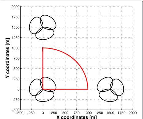
In this section, simulation results for various scenarios are presented and discussed. We assume that all BSs in the network have a three-sector configuration where each sector belongs to a cell with identical coverage area and transmit power. The considered network is composed of three BSs as shown in Figure 2. The cell radius is assumed to be 1 km for all cells. Sectoral antennas are modeled by the antenna model described in Section 2. BSs are located at Cartesian coordinates [0, 0], [1500, 0], and [0, 1500] in meters. In order to evaluate the effect of the restric-tions mentioned in the GSM and UMTS specificarestric-tions on the performance of the proposed algorithm, two cases for the RSS measurements are considered separately. In the first case, exact measurements are used in the algo-rithm. In the second case, measurements are truncated if they are below or above the threshold values mentioned in the standards. In the simulations, it is assumed that BS located at coordinates [0, 0] is the serving cell and the MS does not change its serving cell (i.e., no handover occurs). At each realization, the MS point MS=[x,y] is generated randomly with a uniform distribution inside the area in the first quadrant of the Cartesian coordinates which is bounded by a circle centered at [0, 0] as in Figure 2.
The proposed algorithm computes the ML estimate of the MS position using the RSS measurements and concur-rently calibrates the PLE parameters of the channels occu-pied by different BSs. Recall that this algorithm is referred to as RSS-MPLE algorithm. In order to demonstrate the
improvement on the positioning accuracy provided by the RSS-MPLE algorithm, its performance is compared with those of other algorithms, such as RSS with single PLE algorithm (RSS-SPLE) [46], which finds and calibrates a single PLE for all channels, and RSS with known PLE algo-rithm (RSS-KPLE) [18] in which PLE values are known as a priori. Furthermore, the Cramer-Rao bound has been evaluated and compared with the RMSE results of the proposed algorithm.
4.1 Effect of truncated RSS measurements
RSS measurements below−110 dBm and above−48 dBm are truncated in GSM systems. In Figure 3, the effect of such truncation of RSS measurements in the perfor-mance of the proposed algorithm is investigated. The case in which all BSs have the same PLE value, i.e., α1=α2=α3=3, is considered in this simulation, during which RSS-MPLE and RSS-KPLE algorithms are operated both with truncated and original RSS measurements. The truncated measurements represent all RSS measurements below−110 dBm and above−48 dBm. In Figure 3 (and the subsequent figures in the paper), the following legend clarification is necessary to better interpret the results:
• ‘Truncated RSS are omitted’ means that RSS measurement are truncated and measurements below−110dBm and above−48dBm are not used in the simulations.
• ‘Truncated RSS are used’ means that RSS
measurements being truncated and measurements below−110dBm and above−48dBm are used in the simulations.
−500 −250 0 250 500 750 1000 1250 1500 1750 2000 −500
−250 0 250 500 750 1000 1250 1500 1750 2000
X coordinates [m]
Y coordinates [m]
0 1 2 3 4 5 6 7 8 9 10 0
100 200 300 400 500 600
Shadow Fading Standard Deviation [dB]
Positioning RMSE [m]
RSS−MPLE, Truncated RSS are omitted. RSS−SPLE, Truncated RSS are omitted. RSS−MPLE, Truncated RSS are used. RSS−KPLE, Truncated RSS are omitted. RSS−MPLE,RSS are not truncated. RSS−KPLE,RSS are not truncated.
Figure 3Effect of RSS truncation on position RMSE.When PLE values for all BSs are 3 forσvbetween 0 to 10.
• ‘RSS are not truncated’ means that RSS measurements are not truncated.
From Figure 3, we note that the positioning RMSE obtained with RSS-MPLE algorithm does not exceed 20 m even forσv= 10 if RSS measurements are not truncated. On the other hand, truncation of RSS measurements dra-matically degrades the performance of both RSS-MPLE and RSS-KPLE algorithms due to the decrease in the number of RSS measurements, i.e., the performance of the proposed algorithm is expected to improve with an increase in the number of available measurements.
Since the truncated measurements represent all RSS measurements below −110 dBm and above −48 dBm, they introduce a large bias in the position estimate when incorporated in the RSS measurement set. Because of this, positioning accuracy of the RSS-MPLE algorithm severely degrades when the truncated RSS measurements are not omitted. Compared to the RSS-MPLE algorithm,
the RSS-KPLE algorithm performs better for all σv val-ues when truncated RSS measurements are used. This is an expected result since RSS-MPLE algorithm estimates PLE values in addition to the coordinates with the same number of RSS measurements.
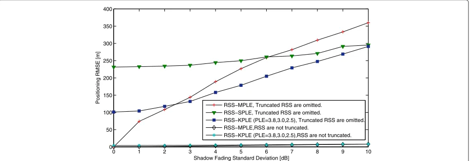
4.2 Effect of inaccurate knowledge of PLE values
In this subsection, the effect of inaccurate PLE values on positioning accuracy is examined and depicted in Figure 4. Throughout the simulation, the PLE valuesα1=3.5,α2= 2.7, andα3 = 2.3 are used in the RSS-KPLE algorithm, whereas actual PLE values areα1 = 3.8,α2 = 3.0, and α3=2.6. Simulations are carried out with both truncated and exact RSS measurements. As shown in Figure 4, the RSS-MPLE algorithm outperforms the rivals under mild shadow fading since the proposed algorithm is capable of adapting PLE values in real time. On the other hand, the PLE inaccuracy has a drastic effect on positioning accu-racy of RSS-KLPLE. Asσvincreases, the adverse effect of
0 1 2 3 4 5 6 7 8 9 10
0 50 100 150 200 250 300 350 400
Shadow Fading Standard Deviation [dB]
Positioning RMSE [m]
RSS−MPLE, Truncated RSS are omitted. RSS−SPLE, Truncated RSS are omitted.
RSS−KPLE (PLE=3.8,3.0,2.5), Truncated RSS are omitted. RSS−MPLE,RSS are not truncated.
RSS−KPLE (PLE=3.8,3.0,2.5),RSS are not truncated.
0 1 2 3 4 5 6 7 8 9 10 0
50 100 150 200 250 300 350 400
Shadow Fading Standard Deviation [dB]
Positioning RMSE [m]
RSS−MPLE, Truncated RSS are omitted. RSS−SPLE, Truncated RSS are omitted. RSS−KPLE, Truncated RSS are omitted. RSS−MPLE,RSS are not truncated. RSS−KPLE,RSS are not truncated.
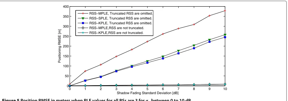
Figure 5Position RMSE in meters when PLE values for all BSs are 3 forσvbetween 0 to 10 dB.
the inaccurate PLE values diminishes since shadow fading becomes the main error source.
4.3 Effect of distinct PLE values
This subsection focuses on the performance analysis of RSS-MPLE, RSS-SPLE, and RSS-KPLE algorithms under different channel conditions. In the first scenario, it is assumed that all channels have the same PLE value. In the second scenario, PLE values differ for channels occupied by different BSs.
4.3.1 Equalα1,α2, andα3
Let us first consider the rather unrealistic case where all BSs (i.e., all channels) are assumed to have the same PLE value which is equal to three (see Figures 5 and 6). In Figure 5, the RMSE for the positioning algorithms of interest is shown. Since PLE values of all channels are identical, the RSS-SPLE algorithm is expected to outper-form the RSS-MPLE algorithm for the same number of
0 100 200 300 400 500 600
0 0.1 0.2 0.3 0.4 0.5 0.6 0.7 0.8 0.9 1
Position Error [m
P(Position Error < x )
RSS−MPLE, Truncated RSS are omitted. RSS−SPLE, Truncated RSS are omitted. RSS−KPLE, Truncated RSS are omitted.
[
Figure 6CDF of positioning error forσv=6dB with PLE values
ofα1=3,α2=3, andα3=3.
RSS measurements, which is indeed the case as depicted in Figure 5.
To evaluate the RSS-MPLE and RSS-SPLE algorithms with respect to the FCC requirements, the positioning error cumulative distribution function (CDF) is shown in Figure 6 forσv=6 dB, which is a realistic value in a micro-cellular environment [31]. The RSS-SPLE and RSS-KPLE algorithms satisfy the FCC requirements, which mandate 67% CERP within 100 m and 95% CERP within 300 m. Although the RSS-MPLE algorithm does not satisfy the FCC requirements, this algorithm offers a solution for environments that possess distinct and variable PLEs.
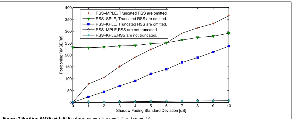
4.3.2 Distinctα1,α2, andα3
From Figure 5, it is seen that the RSS-SPLE algorithm has good performance when all PLEs are equal. How-ever, if BSs have differentαvalues, the RSS-MPLE algo-rithm is expected to outperform the rival algoalgo-rithms since each PLE is treated separately in the RSS-MPLE algo-rithm (see Figures 7 and 8). Moreover, asσv increases, the gap between the positioning RMSE of the RSS-MPLE and RSS-SPLE algorithms closes since the error variance of the α estimates obtained with RSS-MPLE algorithm increases. Such a scenario is simulated for BSs that have different PLE values, i.e., for α1 = 3.5, α2 = 2.7, and α3=2.3.
0 1 2 3 4 5 6 7 8 9 10 0
50 100 150 200 250 300 350 400
Shadow Fading Standard Deviation [dB]
Positioning RMSE [m]
RSS−MPLE, Truncated RSS are omitted. RSS−SPLE, Truncated RSS are omitted. RSS−KPLE, Truncated RSS are omitted. RSS−MPLE,RSS are not truncated. RSS−KPLE,RSS are not truncated.
Figure 7Position RMSE with PLE values.α1=3.5,α2=2.7, andα3=2.3.
RSS-KPLE algorithms are close even when PLE values vary. Thus, RSS-MPLE algorithm satisfies the require-ments for a position estimate with low error variance, independent from unknown propagation parameters, i.e., σv and α values. The positioning error CDF shown in Figure 8 indicates that the accuracy of mobile positioning can substantially be improved by employing the RSS-MPLE algorithm.
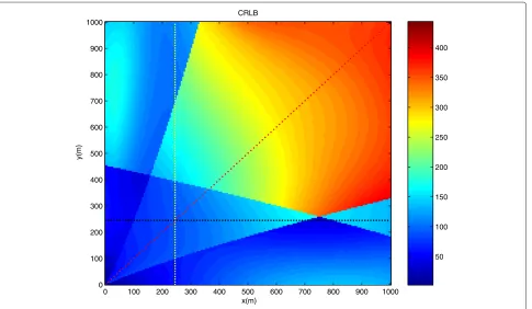
4.4 CRB performance evaluation
In this subsection, we evaluate the CRB bound for the equal PLE case and depict the positioning RMSE for the proposed RSS-MPLE algorithm in Figure 9. From Figure 9, it is noted that the RMSE is relatively high in the middle area, while it shows better results at bound-ary areas. Actually, this is expected due to the pattern
contribution in location estimation since more signal measurements are available for such cases. Figure 10 depicts the CRB results for the same scenario of the pro-posed algorithm RSS-MPLE. From Figures 9 and 10, it can be concluded that the performance degrades up to 450 m in RMSE and 400 m in CRB. Moreover, it is clearly seen that the radiation pattern has a significant effect on location estimation.
5 Conclusions
In this paper, a practical positioning method that can be implemented in mobile networks with simple modi-fications in the existing infrastructure is presented. The proposed method, the so-called RSS-MPLE, is based on RSS measurements and jointly estimates the MS position and the propagation parameters, namely the PLE value of
0 100 200 300 400 500 600
0 0.1 0.2 0.3 0.4 0.5 0.6 0.7 0.8 0.9 1
Position Error [m]
P(Position Error < x ) RSS−MPLE, Truncated RSS are omitted.
RSS−SPLE, Truncated RSS are omitted. RSS−KPLE, Truncated RSS are omitted.
x(m)
y(m)
RMSE
0 100 200 300 400 500 600 700 800 900 1000
0 100 200 300 400 500 600 700 800 900 1000
50 100 150 200 250 300 350 400 450
Figure 9Positioning RMSE in meters whileα=3for all BSs.
x(m)
y(m)
CRLB
0 100 200 300 400 500 600 700 800 900 1000
0 100 200 300 400 500 600 700 800 900 1000
50 100 150 200 250 300 350 400
the measurement channel. The RSS-MPLE method does not need a training period to estimate the PLE value of the channel. The most significant feature of the pro-posed RSS-MPLE algorithm is its ability to separately calibrate the PLE value of each channel occupied by dif-ferent BSs. Moreover, the RSS-MPLE algorithm incor-porates the antenna radiation pattern information that provides additional improvement in positioning accuracy. Via extensive simulations, the performance of the pro-posed method has been compared with those of the existing algorithms in terms of positioning RMSE, bias, availability, and CERP under different environmental con-ditions by changing PLE and SNR values. Simulation results indicate that the RSS-MPLE algorithm is robust against variations in the PLE values under different environment conditions.
6 Appendix
6.1 Cramer-Rao bound for the three BS case
The components of the Fisher information matrix are given as below:
Acknowledgements
The authors would like to thank the referees for their constructive comments which improved the exposition of the paper.
The authors dedicate this article in memory of one of its co-authors, Frederic Kerem Harmanci, who passed away between the completion of his article and its publication.
Received: 13 October 2012 Accepted: 16 June 2013 Published: 26 June 2013
References
1. JJ Caffery,Wireless Location in CDMA Cellular Radio Systems. (Springer, Heidelberg, 2000)
2. IEEE P802.15.4a/D4,Part 15.4: Wireless Medium Access Control(MAC) and Physical Layer (PHY) Specifications for Low-Rate wireless personal area networks (LR-WPANs): Amendment of IEEE Std 802.15.4, July 2006. (IEEE, Piscataway, 2006)
3. FC Commission,Revision of the Commission’s Rules to Ensure Compatibility with Enhanced 911 Emergency Calling Systems, FCC 94-102.
(FC Commission, Washington DC, 1996)
4. J Borkowski, J Niemela, J Lempiäinen, Cellular location techniques supporting A-GPS positioning. IEEE Vehicular Technol. Conf.
1, 429–433 (2005)
5. F Gustafsson, F Gunnarsson, Mobile positioning using wireless networks: Possibilities and fundamental limitations based on available wireless network measurements. IEEE Signal Process. Mag.22(4), 41–53 (2005) 6. K Cheung, H So, W-K Ma, Y Chan, Least squares algorithms for
time-of-arrival-based mobile location. IEEE Trans. Signal Process.
52(4), 1121–1130 (2004)
7. BJ Dil, PJM Havinga, inAustralasian Telecommunication Networks and Applications Conference, ATNAC 2010(Auckland, 31 October – 3 November 2010)
8. B Lakmali, D Dias,Database correlation for GSM location in outdoor & indoor environments. The 4th International Conference on Information and Automation for Sustainability, Colombo, 12-14 December 2008. (IEEE, Piscataway, 2008), pp. 42–47
9. S Ahonen, H Laitinen, Database correlation method for UMTD location. IEEE Vehicular Technol. Conf.4, 2696–2700 (2003)
10. M Spirito, A Mattioli, Preliminary experimental results of a GSM mobile phones positioning system based on timing advance. IEEE Vehicular Technol. Conf.4, 2072–2076 (1999)
11. M Spirito, On the accuracy of cellular mobile station location estimation. IEEE Trans. Vehicular Technol.50(3), 674–685 (2001)
12. M Khalaf-Allah, Nonparametric Bayesian filtering for location estimation, position tracking and global localization of mobile terminals in outdoor wireless environments. EURASIP J Adv. Signal Process.2008, 1–14 (2008) 13. J Borkowski, J Lempiäinen,Pilot correlation positioning method for urban
UMTS networks. Proceedings of the 11th European Wireless Conference, Nicosia, 10–13 April 2005. vol. 2. (IEEE, Piscataway, 2005), pp. 465–469 14. W Pan, J Wu, Z Jiang, Y Wang, X You,Mobile position tracking by
TDOA-Doppler hybrid estimation in mobile cellular system, IEEE International Conference on Communications, Glasgow, 24–28 June 2007. (IEEE, Piscataway, 2007), pp. 4670–4673
15. O Türkyilmaz, F Alagöz, G Gür, T Tugcu, Environment-aware location estimation in cellular networks. EURASIP J. Adv. Signal Process.
2008, 276456 (2008)
16. A Sayed, A Tarighat, N Khajehnouri, Network-based wireless location: challenges faced in developing techniques for accurate wireless location information. IEEE Signal Process. Mag.22(4), 24–40 (2005)
17. J Borkowski, J Lempiäinen, Practical network-based techniques for mobile positioning in UMTS. EURASIP J. Appl. Signal Process.2006, 012930 (2006)
18. K Budka, D Calin, B Chen, D Jeske, A Bayesian method to improve mobile geolocation accuracy. IEEE Vehicular Technol. Conf.2, 1021–1025 (2002) 19. KMK Chu, KRPH Leung, Ng JK-Y, CH Li,Locating mobile stations with
statistical directional propagation model in AINA ’04. Proceedings of the 18th International Conference on Advanced Information Networking and Applications, Washington, 29 - 31 March 2004.
(IEEE, Piscataway, 2004), pp. 230–235
20. Y Qi, H Kobayashi, Cramer-Rao Lower bound for geolocation in non-line-of-sight environment. IEEE Int. Conf. Acoustics, Speech, Signal Process. (ICASSP).3, 2473–2476 (2002)
21. R Yamamoto, H Matsutani, H Matsuki, T Oono, H Ohtsuka, Position location technologies using signal strength in cellular systems. IEEE Vehicular Technol. Conf.4, 2570–2574 (2001)
22. M Aso, T Saikawa, T Hattori, Maximum likelihood location estimation using signal strength and the mobile station velocity in cellular systems. Vehicular Technol. Conf.2, 742–746 (2003)
23. J Zhou, J-Y Ng,A data fusion approach to mobile location estimation based on ellipse propagation model within a cellular radio network, The 21st International Conference on Advanced Information Networking and Applications Niagara Falls, 21 - 23 May 2007.
(IEEE, Piscataway, 2007), pp. 459–466
24. M Akar, U Mitra, Variations on optimal and suboptimal handoff control for wireless communication systems. IEEE J. Selected Areas Commun.
19(6), 1173–1185 (2001)
25. L Mihaylova, D Angelova, S Honary, D Bull, N Canagarajah, B Ristic, Mobility tracking in cellular networks using particle filtering. IEEE Trans. Wireless Commun.6(10), 3589–3599 (2007)
26. K Achutegui, J Rodas, CJ Escudero, J Miguez,A model-switching sequential Monte Carlo algorithm for indoor tracking with experimental RSS data. The International Conference on Indoor Positioning and Indoor Navigation (IPIN), Zurich, 15–17 September 2010.
(IEEE, Piscataway, 2010), pp. 1–8
27. J Turkka, M Renfors,Path loss measurements for a non-line-of-sight mobile-to-mobile environment The 8th International Conference on ITS Telecommunications, Phuket, 24–24 October 2008.
(IEEE, Piscataway, 2008), pp. 274–278
28. S Srinivasa, M Haenggi,Path loss exponent estimation in large wireless networks. (CERN Document Server, Meyrin, 2008)
29. J Shirahama, T Ohtsuki,RSS-based localization in environments with different path loss exponent for each link. IEEE Vehicular Technology Conference, Singapore, 11–14 May 2008. (IEEE, Piscataway, 2008), pp. 1509–1513 30. I Popescu, D Nikitopoulos, P Constantinou, I Nafornita,ANN prediction
models for outdoor environment. IEEE 17th International Symposium on Personal, Indoor and Mobile Radio Communications, Helsinki, 11–14 September 2006. (IEEE, Piscataway, 2006), pp. 1–5
31. T Rappaport,Wireless Communications. (Prentice Hall PTR, New Jersey, 2002)
32. V Erceg, LJ Greenstein, SY Tjandra, SR Parkoff, A Gupta, B Kulic, AA Julius, An empirically based path loss model for wireless channels in suburban environments. IEEE J. Selected Areas Commun.17(7), 1999–1205 (1999) 33. K Martinez, JK Hart, R Ong, Environmental sensor networks. Computer
37, 50–56 (2004)
34. LJ Greenstein, V Erceg, Gain reductions due to scatter on wireless paths with directional antennas. IEEE Commun. Lett.3(6), 169–171 (1999) 35. PF Wilson, PB Papazian, MG Cotton, Y Lo,Advanced antenna test bed characterization for wideband wireless communications, NTIA Technical report. (US Department of Commerce, Washington DC, 1999) 36. TA Rahman, GB Ser, Propagation measurement in IMT-2000 band in
Malaysia environment. TENCON 2000.1, 77–81 (2000)
37. S-W Wang, I Wang,Effects of soft handoff, frequency reuse and non-ideal antenna sectorization on CDMA system capacity. 43rd IEEE Vehicular Technology Conference, Secaucus, 18–20 May 1993. (IEEE, Piscataway, 1993), pp. 850–854
38. A Vavoulas, N Vaiopoulos, DA Varoutas, A Chipouras, G Stefano, Performance improvement of fixed wireless access networks by conjunction of dual polarization and time domain radio resource allocation technique. Int. J Commun. Syst.24, 483–491 (2010) 39. J Park, JW Jang, S-G Park, W Sung, Capacity of sectorized distributed
networks employing adaptive collaboration from remote antennas. IEICE Trans.E93-B, 3534–3537 (2010)
40. D Runyon, Optimum directivity coverage of fan-beam antennas. IEEE Antennas Propagation Mag.44(2), 66–70 (2002)
41. SM Kay,Fundamentals of Statistical Signal Processing: Estimation Theory. (Prentice Hall PTR, New Jersey, 1993)
43. J-Y Fan, Y-X Yuan, On the quadratic convergence of the
Levenberg-Marquardt method without nonsingularity assumption. Computing.74, 23–39 (2005)
44. K Madsen, HB Nielsen, O Tingleff,Methods for Non-linear Least Squares Problems. (Informatics and Mathematical Modelling Technical University of Denmark, Lyngby, 2004)
45. K Pahlavan, A Levesque,Wireless Information Networks. (John Wiley and Sons, Inc., New York, 1995)
46. X Li, RSS-based location estimation with unknown pathloss model. IEEE Trans. Wireless Commun.5(12), 3626–3633 (2006)
doi:10.1186/1687-1499-2013-178
Cite this article as:Zeytinciet al.:Location estimation using RSS
mea-surements with unknown path loss exponents.EURASIP Journal on Wireless Communications and Networking20132013:178.
Submit your manuscript to a
journal and benefi t from:
7Convenient online submission
7 Rigorous peer review
7Immediate publication on acceptance
7 Open access: articles freely available online
7High visibility within the fi eld
7 Retaining the copyright to your article