R E S E A R C H
Open Access
Diversity analysis, code design, and tight
error rate lower bound for binary joint
network-channel coding
Dieter Duyck
1*, Michael Heindlmaier
2, Daniele Capirone
3and Marc Moeneclaey
1Abstract
Joint network-channel codes (JNCC) can improve the performance of communication in wireless networks, by combining, at the physical layer, the channel codes and the network code as an overall error-correcting code. JNCC is increasingly proposed as an alternative to a standard layered construction, such as the OSI-model. The main
performance metrics for JNCCs are scalability to larger networks and error rate. The diversity order is one of the most important parameters determining the error rate. The literature on JNCC is growing, but a rigorous diversity analysis is lacking, mainly because of the many degrees of freedom in wireless networks, which makes it very hard to prove general statements on the diversity order. In this article, we consider a network with slowly varying fading
point-to-point links, where all sources also act as relay and additional non-source relays may be present. We propose a general structure for JNCCs to be applied in such network. In the relay phase, each relay transmits a linear transform of a set of source codewords. Our main contributions are the proposition of an upper and lower bound on the diversity order, a scalable code design and a new lower bound on the word error rate to assess the performance of the network code. The lower bound on the diversity order is only valid for JNCCs where the relays transform only two source codewords. We then validate this analysis with an example which compares the JNCC performance to that of a standard layered construction. Our numerical results suggest that as networks grow, it is difficult to perform
significantly better than a standard layered construction, both on a fundamental level, expressed by the outage probability, as on a practical level, expressed by the word error rate.
Keywords: Joint network-channel coding, Slow Rayleigh fading, Diversity, Low-density parity-check codes
1 Introduction
Point-to-point communication has revealed many of its secrets. Driven by new applications, research in wire-less communication is now focusing more on the opti-mization of communication in wireless networks. For example, the joint operation of multiple network layers can be optimized, denoted as cross-layer design [1,2], thereby leaving the classical layered architectures, such as the seven-layer open systems interconnect (OSI) model ([3], p. 20). Another example of network optimization is cooperative communication, where multiple nodes in the network cooperate to improve their error performance.
*Correspondence: [email protected]
1Department of Telecommunications and Information processing, Ghent University, St-Pietersnieuwstraat 41, B-9000 Gent, Belgium
Full list of author information is available at the end of the article
Cooperation may occur in many forms at different lay-ers, e.g., cooperative channel coding at the physical layer and network coding at the network layer. Network cod-ing refers to the case where the intermediate nodes in the network are allowed to perform encoding operations over multiple received streams from different sources. In a standard layered construction, the decoding of the net-work code is performed at the netnet-work layer, after the point-to-point transmissions have been decoded at the physical layer. Channel coding refers to the case where nodes perform coding over one point-to-point wireless link only. Cooperative channel coding is achieved by let-ting one or more relays transmit redundant bits for one source at a time. Usually, channel coding and network coding are studied separately (e.g., [4-6] for cooperative channel coding and [7-11] for network coding).
Standard linear network coding consists of taking lin-ear combinations of several source packets. In general, non-binary coefficients are used in the linear combina-tions. In JNCC, cooperative channel coding (e.g., decode and forward [12]) and cross-layer design are combined, by using the network code for decoding at the physi-cal layer. The rationale behind JNCC is to improve the joint error rate performance (i.e., the average error rate performance over all users participating in the network) by letting the redundancy of the network code help to decode the noisy channel output [13]. In that case, a joint optimization of the network and channel code is useful. For example, one can opt to let the network and chan-nel code be represented by one parity-check matrix of a binary code, referred to as joint network-channel coding (JNCC). Hence, the coefficients multiplying the packets in the case of standard linear network coding are replaced by matrices in the case of JNCC.
Mostly, the two most important performance metrics are(R,Pe), whereRis the information rate andPeis the error rate. Here, we consider a fixed information rateR, so that the aim is to minimizePefor a given point-to-point channel quality, expressed byγ, the signal-to-noise ratio (SNR) per symbol. Expressing the asymptotic (for largeγ) error rate asPe = gγ1d, whereganddare defined as the coding gainand thediversity order, respectively, improv-ing the performance refers to maximizimprov-ing firstdand then g (becaused has the larger impact). Next to minimizing the error rate, scalability of the code design (e.g., to larger networks) is also an important criterion often recurring in the literature. JNCC is increasingly proposed as an alter-native to a standard layered construction, such as the OSI model. However, it must be verified that important met-rics, such as the diversity order d and the scalability to large networks, are not negatively affected.
Binary JNCC received much attention in the last years. Pioneering articles [14,15] designed turbo codes and LDPC codes, respectively, for the multiple access relay channel (MARC) and for the two-way relay channel [16]. However, the code design was not immediately scalable to general large networks and did not contain the required structure to achieve full diversity. The study of Hausl et al. [14-16] was followed by the interesting study of Bao et al. [17], presenting a JNCC that is scalable to large networks. However, this JNCC was not structured to achieve full diversity and has weak points from a coding point of view [18]. A deficiency in the literature, for general networks with a number of sources and relays, is the lack of a detailed diversity analysis in the case that the sources can act as a relay (which is for example the model assumed by [17]). The effect of the parameters of the JNCC on the diversity order is in general not known, because of the many degrees of freedom in such networks. Related to this, we mention [19,20], where the authors designed a
JNCC for the case where the sources cannot act as a relay, but other nodes play the role of relay to communicate to one destination. As the source nodes are excluded to act as a relay node in this model, the diversity analysis in [19,20] is different from ours.
In this article, we consider a JNCC where the network code forms an integral part of the overall error-correcting code, that is used at the destination to decode the informa-tion from the sources. The rest of the article is organized as follows. In Section ‘Diversity analysis of JNCC’, we per-form a diversity analysis, leading to an upper bound on the diversity order of any linear binary JNCC following our system model, and to a lower bound on the diversity order for a particular subset of linear binary JNCCs. The upper and lower bound depend on the parameters of the JNCC and can be used to verify whether a particular JNCC has the potential to achieve full diversity on a certain net-work. Second, in Section ‘Practical JNCC fornur = 2’, a specific JNCC of the LDPC-type is proposed that achieves full diversity for a well identified set of wireless networks. The scalability of this specific JNCC to large networks is discussed. The coding gain cis not considered in the body of the article and the parameters of our proposed code may be further optimized by applying techniques such as in [19], to maximizec. To assess the performance of the proposed JNCC, we determine the outage proba-bility, a well known lower bound of the word error rate, in Section ‘Lower bound for the WER’. We also present a tighter word error rate lower bound in Section ‘Calcu-lation of a tighter lower bound on WER’, that takes into account the particular structure of the JNCC. In Section ‘Numerical results’, the numerical results corroborate the established theory. We also briefly comment on the cod-ing gain achieved by the proposed JNCC and conclusions are drawn for different classes of large networks.
This article extends the study, published in [18], by also considering non-perfect source-relay channels, by consid-erably extending the diversity analysis, by providing an achievability proof for the diversity order of the proposed JNCC, by clearly indicating the set of wireless networks where the proposed JNCC is diversity-optimal, by provid-ing a tighter lower bound on the word error rate, and by providing more numerical results.
2 Joint network-channel coding
We first illustrate joint network-channel coding by means of a simple example. Consider two sources orthogonally broadcasting a vector of symbols, mapped from the binary vectorss1ands2, respectively, to a relay and a destination.
This channel is denoted as a multiple access relay chan-nel (MARC) in the literature. Supposing that the relay is able to decode the received symbols, the relay computes a binary vectorr1, which is mapped to symbols and
trans-mitted to the destination. The relation between all bits is expressed by the JNCC, whose parity-check matrix has the following general form,
H
s1 s2 r1
Hp 0 0
0 Hp 0
0 0 Hp
H11 H21 H1
.
(1)
The matrix Hp represents the parity-check matrix for the point-to-point channel code. Each of the binary vec-torss1, s2, and r1, can be separately decoded using this
code. The bottom part ofHrepresents the GLNC, which we denote asHGLNC =[H11H21H1]. It expresses the
rela-tion betweenr1,s1, ands2. More specifically, we have
H1r1=H11s1+H21s2. (2)
Note that GLNC includes standard network codes used in an OSI communication model as a special case. In the latter case, the matricesHjiandHi(considering more than one relay in general) are identity matrices or all-zero matrices, so that the network code simplifies to the relay packet being a linear combination of source packets, also expressed as XORing of packets or symbol-wise addition of packets.
Ideally, the overall matrixHconforms optimized degree distributions that specify the LDPC code. When the chan-nels between sources and relay are perfect, we can drop the first three sets of rows and only keep the GLNC, rep-resented byHGLNC; in this case the information bits of the
code ares1ands2, andr1contains the parity bits. This is
still a JNCC as the redundancy in the network code is used to decode the received symbols on the physical layer at the destination. In [21,22], it is proved that the matricesHpdo not affect the diversity order in the case of the MARC.
3 System model
We consider wireless networks withms sources directly communicating to a common destination (e.g., cellphones communicating to a base station). Two time-orthogonal phases are distinguished. In thesource phase, the sources orthogonally broadcast their respective source packet. In the followingrelay phase, the relays orthogonally broad-cast their respective packet. All considered sources over-hear each other during the source phase, and act as relay in the relay phase. Other nodes, not acting as a source, might be present in the network (i.e., overhearing the sources) and also act as relay. Hence, we consider a total ofmrrelays, wheremr≥ms. This general network model, which is practically relevant as it fits many applications, is adopted in, e.g., [17]. Take for example any large network and consider a volume in space (cf. picocells or femtocells) where all nodes can overhear each other. These nodes formsub-networksand can be modeled by our proposed model. Note that in the literature, sometimes other mod-els are assumed, such as theM−N−1 model [19,20], where Msources are helped byN relays (the relays are nodes different from the sources) to communicate to one destination.
All devices have one antenna, are half-duplex and trans-mit orthogonally using BPSK modulation. TheK infor-mation bits of each source are encoded viapoint-to-point channel codes into a systematic codeword, denoted as source codeword, of length L, expressed by the column vectorsus for userus,us ∈[ 1,. . .,ms]. The parity-check matrix of dimension(L−K)×Lof this point-to-point codeword is denoted byHp, which is the same for each userus, so thatHpsus = 0for allus. In the relay phase, each relayur,ur ∈[ 1,. . .,mr], transmits a point-to-point codewordrur of length Lto the destination, also satisfy-ingHprur = 0. Hence, all slots have equal duration, the coding rate of the point-to-point channels is Rc,p = KL, and the overall coding rate isRc= msK
(ms+mr)L =Rc,p ms ms+mr. We define the fraction of source transmissions in the total number of transmissions as the network coding rateRn=
ms
ms+mr, so that Rc = Rc,pRn. The overall codeword of length(ms+mr)Lis expressed by the column vector
x=sT1 . . .sTmsrT1. . .rTms. . .rTmrT. (3)
The destination declares a word error if it can not per-fectly retrieve all msK information bits, and the overall word error rate is denoted byPew.
that is longer than the duration of the source phase and the relay phase, so that the fading gain between two net-work nodes takes the same value during both phases. We denote the fading gain from nodeuto the destination as
αu, withE[αu2]= 1. All point-to-point channels have the same average signal-to-noise ratio (SNR), denoted byγ. Differences in average SNR between the channels would not alter the diversity analysis, on the condition that the large SNR behavior inherent to a diversity analysis refers to allb SNRs being large. Denoting the received symbol vector at the destinationcin timeslotiasyi, the channel equation is
yus=αussus+nus, us=1,. . .,ms yms+ur =αurrur+nms+ur, ur=1,. . .,mr,
(4)
where ni ∼ CN(0,γ1I) is the noise vector in timesloti, sus =2sus−1 andrur =2rur−1 (BPSK modulation).
Hence, at the destination, each of thems independent fading gains between the sources and the destination affects 2Lbits (Lbits in the source phase andLbits in the relay phase) and each of mr −ms fading gains between the non-source relays and the destination affects Lbits, assuming that all mr relays could decode the messages received from the sources. Hence, from the point of view of the destination, the overall codeword is transmitted on a block fading (BF) channel withmrblocks, each affected by its own fading gain, wheremsblocks have length 2Land mr−msblocks have lengthL. This notion will be essen-tial in the subsequent diversity analysis (Section ‘Diversity analysis of JNCC’).
In the source phase, relay ur attempts to decode the received symbols from sources belonging to the decod-ing set S(ur). The users that are successfully decoded at relay ur are added to its retrieval set, denoted by
R(ur), R(ur) ⊂ S(ur), with cardinalitylur. Next, in the relay phase, relay ur transmits a relay packet, which is a linear transformation of nur source codewordsd origi-nated by the sources from the transmission setT(ur) =
{u1, . . ., unur} of relay ur, with T(ur) ⊂ R(ur). If lur < nur, then relay ur does not transmit anything. In Section ‘Diversity analysis of JNCC ’, we show thatnur is an important parameter that strongly affects the diversity order.
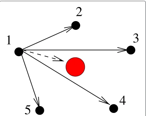
For example, user 3 attempts to decode the messages from users 1, 2, and 5, and succeeds in decoding the messages from users 1 and 5 from which a linear trans-formation is computed. Hence,S(3) = {1, 2, 5},R(3) = T(3) = {1, 5}, l3 = n3 = 2. Because the channel
between a node and the destination remains constant dur-ing both source and relay phases, a relay has no interest in including its own source message inS(ur).
Using the transmission set for each relay, the GLNC in Equation (2) generalizes to
Hurrur =
us∈T(ur) Hur
ussus, (5)
where the matricesHur andH ur
us are of dimensionK×L. Hence, each transmitted relay codeword rur is a linear transformation ofnur source codewords. The superscript ur in Huusr indicates that the vector sus is in general not transformed by the same matrix for all relays ur where us ∈ T(ur). The overall parity-check matrix H is thus expressed as
H=
Hc HGLNC
, (6)
whereHcis block diagonal withHpon its diagonal, repre-senting the channel code, and
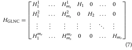
HGLNC=
⎡ ⎢ ⎢ ⎢ ⎢ ⎢ ⎣
H11 . . . Hm1s H1 0 . . . 0
H12 . . . Hm2s 0 H2 . . . 0
..
. ... ... ... ... . .. ... Hmr
1 . . . Hmmsr 0 0 . . . Hmr
⎤ ⎥ ⎥ ⎥ ⎥ ⎥ ⎦
(7)
represents the GLNC.
Table 1 provides an overview of the notation presented in the system model.
Table 1 Overview of notation for JNCC for larger networks
ms Number of sources mr Number of relays
Rn Network coding rate,Rn= msm+smr
u,ur,us user indices to indicate a user in general, a relay, and a source, respectively
T(ur) Transmission set of relayur
nur |T(ur)|, i.e., the number of sources helped by relayur sus,rur Point-to-point codeword transmitted by sourceus and
relayur, respectively
L Code length of all point-to-point codewords
Hp Parity-check matrix of point-to-point codewords, e.g., Hpsus=0
Rc,p Coding rate of point-to-point codewords
c Overall codeword, that is, the concatenation of all point-to-point codewords
H Parity-check matrix of overall codeword
Rc Coding rate of overall codeword,Rc=Rc,pRn
HGLNC The part ofHthat relates the relay codewordsrurto the
source codewordssus
Hur
4 Diversity analysis of JNCC
Before passing to the actual diversity analysis, we provide the well-known formal definition of the diversity order ([23], Chap. 3).
Definition 1.The diversity order attained by a codeCis defined as
d= − lim
γ→∞ logPew
logγ ,
whereγ is the signal-to-noise ratio.
In other words,Pew ∝ γ−d, where∝denotes
propor-tional to.
In the proofs of propositions in this article, we will often use the diversity equivalence between a BF channel and a block binary erasure channel (block BEC), which was proved in [24,25]. A block BEC channel is obtained by restricting the fading gains in our model to belong to the set{0,∞}, so that a point-to-point channel is either erased or perfect. Denoting the erasure probability Prαur =0 by, a diversity orderdis achieved ifPew ∝dfor small
[26]. A diversity order ofd is thus achievable if there exists no combination ofd−1 erased point-to-point chan-nels leading to a word error. On the other hand, a diversity order of d is not achievable if there exists at least one combination ofd − 1 erased channels leading to word error.
In this section, we present the relation between the diversity orderdand the parameters{nur,ur =1,. . .,mr}, as well as between d and the choice of {T(ur),ur = 1,. . .,mr}. This guides the code design and furthermore, the potential, of a linear binary JNCC satisfying some con-ditions, to achieve full diversity, can be verified without performing Monte Carlo simulations.
We first prove that the diversity order is a function of only the network coding rateRn (Section ‘Diversity as a function of the network coding rate’). We then determine in Section ‘Space diversity by cooperation’ the relation between the diversity order d and the set {nur,ur = 1,. . .,mr}, for any linear binary JNCC expressed as in Equations (6) and (7). The set{nur,ur = 1,. . .,mr} actu-ally determines the maximal spatial diversity that can be achieved by cooperation, leading to an upper bound on the diversity order. In Section ‘A lower bound based on
{T(ur)}fornur = 2’, we propose a lower bound on the diversity order in the case that nur = n = 2, which depends on all transmission sets{T(ur),ur =1,. . .,mr}. In Section ‘Diversity order with interuser failures’, we discuss how the diversity order is affected by interuser failures. Finally, in Section ‘Diversity order in a layered construction’, we briefly comment on the diversity order in a layered construction, such as the OSI model.
4.1 Diversity as a function of the network coding rate
We denote the maximum achievable diversity order by dmax. We will determinedmaxin this section and show that
it only depends on the network coding rateRn= msm+smr. Proposition 1.Under ML decoding, the maximum diversity order dmax that can be achieved by any linear JNCC is
dmax=
⎧ ⎨ ⎩
1+mr
2 , if mr≤2ms 1+mr−ms , if mr>2ms
. (8)
Proof.See Appendix 1.
Note that the maximal diversity order does not depend onL. It can actually be reformulated in the following way:
dmax=
⎧ ⎨ ⎩
1+(1−Rn)(mr+ms)
2 , ifmr ≤2ms 1+mr−(ms+mr)Rn , ifmr>2ms ,
(9)
which formr = ms = mreduces to the maximum diver-sity order for a standard BF channelewithmblocks and coding rateRn[27-29].
Hence, the maximum diversity order does not change when the point-to-point channel coding rateRc,pchanges. This corresponds with our intuition as the parity bits of the point-to-point codes only provide redundancy within one block forming a point-to-point codeword, hence these parity bits cannot combat erasures which affect the com-plete point-to-point codeword. Another consequence is that the maximal diversity order of JNCC cannot be larger than in a layered approach, with the same network coding rate.
In the remainder of the article, full diversity refers to the diversity order being equal to the maximal diversity order, d=dmax, from (8).
4.2 Space diversity by cooperation
We denote the word error rate for each sourceusbyPew,us, which is the fraction of packets where at least 1 of theK information bits from source us is erroneously decoded at the destination. Associated toPew,us, we definedus, so thatPew,us ∝
1
γdus for largeγ. We have that maxuPew,us ≤ Pew≤usPew,us. From Definition 1, it follows that
d=min
us
dus. (10)
Denotetus,us∈ {1,. . .,ms}, as the number of times that source us is included in the transmission set of a relay: tus =
tmin = minustus andtav =
diversity order, as it is the minimal number of channels that convey a source message to the destination.
Proposition 2.For any linear JNCC, applied in our system model, the diversity order d is upper bounded as
d≤dR=1+tmin.
Proof. We use the diversity equivalence between a BF channel and block BEC [24,25]. Assume that the channel between sourceus and the destination is erased. Source us is included in at mosttus transmission sets. Assume that alltuschannels between the relays, that include source us in their transmission set, and the destination are also erased. Then the destination does not receive any infor-mation on source us so that it can never retrieve its message. The probability of occurrence of this event is
1+tus, so thatPew,u
s ≥1+tus, hencedus ≤1+tus. Using Equation (10), we obtain Proposition 2.
Note that the proof of Proposition 2 is based on the assumption that relayuronly considers packets transmit-ted in the source phase for inclusion inS(ur). In the case that relayurcomputes its relay packet also based on pack-ets transmitted by other relays during the relay phase, the diversity order becomes more difficult to analyze.
In Corollary 1, we propose the conditions on tmin so
that the space diversity orderdR is not smaller than the maximum achievable diversity order.
Corollary 1.For any linear JNCC, applied in our system model, full diversity can be achieved only if tmin≥q, where
q=
Proof. The proof follows directly from Propositions 1 and 2.
Given a GLNC, and thus a choice of T(ur), one can verify whether the condition in Corollary 1 holds. In the disaffirmative case, full diversity cannot be achieved. To get more insight for the code design, we consider the sim-plest case of a network code where the cardinality of the transmission set is constant (nur =n).
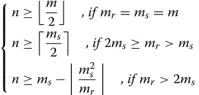
Corollary 2.For any linear JNCC, applied in our system model, with constant nur =n, full diversity can be achieved only if have the necessary condition thatn ≥ qms
mr. As nis an integer, this bound can be tightened, yieldingn≥ms
mrq
. Filling inqfrom Corollary 1 yields Corollary 2.
Table 2 illustrates Corollary 2, showing the set of net-works in which a certain parameternis diversity-optimal, which means that the choice of ndoes not prevent the code to achieve full diversity. In Section ‘Practical JNCC fornur = 2’, we propose a JNCC forn = 2, where taking n = 2 is diversity-optimal in all networks corresponding to bold elements in Table 2.
4.3 A lower bound based on{T(ur)}fornur=2
A certain relay does not help one source only, but a combi-nation of sources, expressed by the transmission setT(ur) for each relayur. In this section, we provide a lower bound on the diversity order, based on the choice of{T(ur),ur = 1,. . .,mr}. If this lower bound and the upper bound in the previous section are tight, the exact diversity order of JNCCs can so be determined, as will be illustrated in Section ‘Practical JNCC fornur =2’.
Based onT(ur),msandmr, we construct the(ms+mr)× mscoding matrixM, where
⎧
to maintain its capability to achieve full diversity
The matrix M expresses the presence of a source-codeword in each transmission, i.e., Mi,us = 1 if sus is considered in transmission i (i = 1,. . .,ms and i = ms+1,. . .,ms+mr correspond to the source and relay transmission phases, respectively). Therefore, the upper part ofMis an identity matrix as each sourceus trans-mits its own codewordsusin the source phase. The matrix M represents what is often called the “coding header” or “the global coding coefficients” in the network coding literature (see e.g., [30]).
Consider a block BEC channel whereeof themrblocks have been erased. The indices of the fading gains corre-sponding to the erased blocks are collected in the setE=
{E1,. . .,Ee},Ei ∈ {1,. . .,mr}). Based onE, we construct ME which corresponds to the subset of transmissions that are not erased, i.e., all rowsEi(ifEi ≤ ms) andms+Ei, user 1 and the destination is erased, so that rows 1 and 4 fromMare dropped:
A simple computer program can compute dM, given
T(ur),msandmr.
Lemma 1.In a JNCC following the form of Equation (6) with ms=mrand constant nur =n=2, the metric dMis at most three.
Proof.Ifms=mrandn=2, then the minimum column weight ofMis smaller than or equal to three. Erasing the three rows whereMi,us = 1, for a certainus correspond-ing to the minimum column weight, leads toME having at least one zero column, and thusrME < ms. By Definition 2,dM<4.
In the next proposition, we provide a lower bound on the diversity order under ML decoding or Belief Propaga-tion (BP) decoding [31]. We denote
Hur
which are square matrices of dimensionL.
Proposition 3.Using ML decoding, the diversity order of a JNCC following the form of Equation (6) with constant nur =n=2, is lower bounded as
d≥dM,
if the matricesHur
us, us∈T(ur),ur ∈ {1,. . .,ms}, have full rank.
Using BP-decoding, the diversity order of a JNCC follow-ing the form of Equation (6) with constant nur =n=2, is
can be solved with BP in the case of only one unknown source-codeword vector.
Proof.See Appendix 2.
We can simplify the condition for BP decoding, stated in Proposition 3, when we assume that the parity bits of point-to-point codes do not have a support inHGLNC, or
said differently, when theL−Kright most columns of the matricesHurandH
ur
usare zeroes. In that case, one iteration in the backward substitution, mentioned in Appendix 2, corresponds to solving theKunknown information bits of suvia the set ofKequations
Hur
In Section ‘Practical JNCC fornur = 2 ’, we propose a JNCC where the parity bits of point-to-point codes do not have a support inHGLNC, so that we take (17) instead
4.4 Diversity order with interuser failures
It is often easier to prove that a particular diversity order is achieved assuming perfect interuser channels (see for example in Section ‘Practical JNCC fornur = 2 ’). Here, we discuss how this diversity order is affected by interuser failures.
Lemma 2.In the case of non-reciprocal interuser chan-nels, any JNCC achieves the same diversity order with or without interuser channel failures.
Proof. See Appendix 3.
In the case of reciprocal interuser channels, the achieved diversity order with interuser failures depends on the transmission sets {T(ur),ur = 1,. . .,mr}. We propose an algorithm to construct {T(ur)} in Section ‘Practical JNCC fornur =2’ and we will then discuss the diversity order with reciprocal interuser channels.
4.5 Diversity order in a layered construction
In a layered construction, such as the standard OSI model, the destination first attempts to decode the point-to-point transmissions. If it can not successfully retrieve the transmitted point-to-point codeword for a particular node-to-destination channel, then it declares a block era-sure, where a block refers to one point-to-point codeword. Denoting this block erasure probability by, we have that
∝ γ1 ([23], Equation (3.157)). If for example e blocks of lengthLare erased, then the decoding corresponds to solving a set of equations witheLunknowns.
Standard linear network coding consists of taking lin-ear combinations of several source packets. In general, non-binary coefficients are used in the linear combina-tions. Hence, packets are treated symbol-wise, which is shown to be capacity achieving for the layered construc-tion [8]. A consequence of this symbol-wise treatment is that the effective block length of the network code reduces toms+mr and the set of equations, that are available at the destination for decoding, is expressed by the coding matrixME. At this block length, ML decoding (which is equivalent to Gaussian elimination at the network layer) has low complexity. Under ML decoding, a sufficient con-dition for successful decoding isrME = ms. Also, for ML decoding, the maximum number of erasurese∗=dM−1 (Definition 2), so that the conditionrME =msis satisfied, is equal to the minimum distance of the non-binary code minus one. The minimal distance is, for a given coding rate, maximum for maximum distance separable (MDS) codes, so thatdMis maximum for MDS codes as well. Also note that random linear network codes are MDS codes with high probability for a sufficiently large field size [32]. Table 3 provides an overview of the notation presented in this diversity analysis.
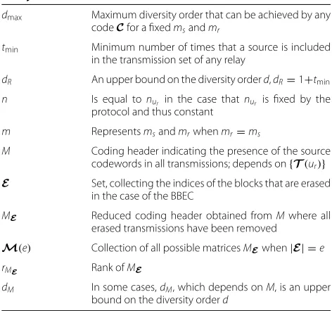
Table 3 Overview of notation introduced in the diversity analysis
dmax Maximum diversity order that can be achieved by any codeCfor a fixedmsandmr
tmin Minimum number of times that a source is included in the transmission set of any relay
dR An upper bound on the diversity orderd,dR=1+tmin
n Is equal tonur in the case thatnur is fixed by the
protocol and thus constant
m Representsmsandmrwhenmr=ms
M Coding header indicating the presence of the source codewords in all transmissions; depends on{T(ur)} E Set, collecting the indices of the blocks that are erased
in the case of the BBEC
ME Reduced coding header obtained fromMwhere all erased transmissions have been removed
M(e) Collection of all possible matricesMEwhen|E| =e
rME Rank ofME
dM In some cases,dM, which depends onM, is an upper bound on the diversity orderd
Tables 1 and 3 indicate the complexity of the analysis of JNCC for large networks.
5 Practical JNCC fornur =2
In the literature, a detailed diversity analysis is most often lacking. Codes were proposed and corresponding numer-ical results suggested that a certain diversity order was achieved on aspecificnetwork. It is sometimes not clear why this diversity order is achieved, and how it would vary if the network or some parameters change. In the previous section, we made a detailed diversity analysis of a JNCC following the form of Equation (6). However, the utility of for example Proposition 3 is limited to JNCCs follow-ing the form of Equation (6) with a constant nur = 2, which suggests that it is very hard to rigorously prove diversity claims in general. However, the modest analy-sis made in Section ‘Diversity analyanaly-sis of JNCC ’ can be applied in some cases and we will show its utility through an example.
We consider networks withms = mr = m ≥ 4 and a JNCC following the form of Equation (6) withnur =n=2 forur = 1,. . .,m. We will rigorously prove that a diver-sity order of three is achieved, using the propositions of Section ‘Diversity analysis of JNCC’. From Table 2, it can be seen that this JNCC is diversity-optimal for m = 4 and m = 5. In Section ‘Numerical results’, we provide numerical results form=5.
Furthermore, taking n = 2 does not impose infeasible constraints on the number of sources in the vicinity of a relay in the case that spatial neighborhoods are taken into account. Next, the theoretical analysis is simpler in the casen = 2. Finally, taking n = 2 allows to reuse strong codes designed for the multiple access relay channel, e.g., in [21,22].
Besides the diversity order, we indicated in Section ‘Introduction’ that scalability is also very important. The JNCC proposed here is scalable to any large network with-out requiring a redesign of the code. This means that we provide an on the fly construction method. The latter is particularly important for self regulating networks. As a node adds itself to the network, it can seamlessly inte-grate to the network. Together with the new symbols sent by the new node, a new JNCC code is formed which still possesses all desirable properties. Finally, note that due to the large block length of JNCC, ML decoding is too com-plex and low-comcom-plexity techniques, such as BP decoding, must be used.
Hence, two properties are claimed: scalability to large networks and a diversity order of three (which is full diver-sity in some cases) under BP decoding. The JNCC code is presented in two steps. First, we present the design of
{T(ur)}and thus the coding matrixM. In a second step (Equation (20)), we specify the matricesHur andH
ur us and we will prove that the scalability and the diversity order of three are achieved.
5.1 First step: design ofT(ur)
The transmission sets{T(ur)}have a large impact on the diversity order. For example, in [18], a random construc-tion was studied (each relay choosesn=2 sources at ran-dom) and it was shown thatE[tus]=2, but Var[tus]=2 as well, so that most probablytmin<2 anddR<3 (Proposi-tion 2). So we need a more intelligent construc(Proposi-tion.
We present an algorithm to determine{T(ur)}, givenms andmr, and we subsequently determine the correspond-ing metricstminanddM. We define the functionfms(x)=
((x−1) modms)+1 which adapts the modulo operation to the range 1≤fms(x)≤ms.
Algorithm 1. Choose transmission setT(ur).
The transmission setT(ur)is expressed via the bottom part of M. An example of such a matrix Mis given in Equation (18) forms=mr=5.
If a node is added as a source node, it adopts the largest source index,ms+1, and relay-only nodes, with indices larger than or equal to ms + 1, increment their index by one. The function fms(x) is updated to the new ms. Note that the algorithm corresponds to a deterministic cooperation strategy, which avoids extra signalling to the destination regarding the code design.
We first consider the case of perfect interuser channels and prove that Algorithm 1 yieldsd = 3 (Corollary 3). We then consider interuser failures and prove that the diversity order is not affected (Lemma 3).
Corollary 3.Having perfect links from sources to relays, the diversity order of a JNCC, with ms = mr and with transmission set constructed via Algorithm 1, achieves a diversity order d = 3using BP-decoding, if, for each ur, Equation (17) can be solved with BP in the case of only one unknown source-codeword vector.
Proof.Because the links between sources and relays are perfect, the relays will never stay silent. In the case that mr =msandnur =2, we have thattmin=tav=2 and so
relaysu1andu2having sourceusin their transmission set (T(u1)andT(u2), respectively) are
u1=fms(us−1),u2=fms(us−2).
Hence, source 1 is included inT(m−1)andT(m), and source 2 is included inT(m)andT(1). Hence, relay trans-missionm−1 can be used to retrieve source 1 and relay transmissionmcan be used to retrieve source 2, as long asm≥4. Hence,ME has full rank. The generalization to any setEsatisfying|E| =2, is straightforward. Therefore, we have thatdM=3.
Next, it can be proved that a JNCC applied in our system model has a diversity order of three, if it has a diversity order of three when all interuser channels are perfect. This is proved in general for non-reciprocal interuser channels in Lemma 2, and here, we consider reciprocal interuser channels.
Lemma 3.A JNCC, with transmission set constructed via Algorithm 1, achieves the same diversity order with or without interuser channel failures when ms > 4or when ms=mr=m≤4.
Proof. See Appendix 4.
For conciseness, we do not consider the other cases, mr >ms≤4.
5.2 Second step: JNCC of LDPC-type
In the first step, we specified{T(ur)}and proved thatdR= dM = 3 ifmr =ms = m> 3. According to Corollary 3, a diversity order of three is achieved under BP decoding if, for eachur, Equation (17) can be solved with BP in the case of only one unknown source-codeword vector. In the second step, we specify the sub matricesHur,H
ur
us,∀ur,us, to satisfy this condition, given that{T(ur)}is constructed according to Algorithm 1.
A simple solution is to replace theKleft most columns in all K ×L sub matrices Hur, H
ur
us, ∀ur,us, by identity matrices. In this case, the joint network channel cod-ing essentially reduces to a layered solution: the source-codewords are decoded at the relays and simply added according to Equation (5). If the network code is used at the physical layer, it has to deal with noise and a more advanced code might be required.
In the literature, a full-diversity close-to-outage per-forming JNCC for the Multiple Access Relay Channel (MARC) has been proposed [21,22], which is a code in the form of Equation (1). These codes are such that the set of equations
H11s1+H21s2+H1r1=0
can be decoded via BP if only one coding vector s1, s2
or r1 is erased and the other coding vectors are
per-fectly known. We denote this JNCC by MARC-JNCC. The matrixHGLNC, MARCof the MARC-JNCC is given by
Equation (A.7) in [21]f: [1ij2ij] andpjdenoting the information bits and the par-ity bits, respectively (j = 1, 2);1ij and2ij each contain
K
2 information bits. However, the parity bits pj are not
involved inHGLNC, MARC. The matricesRi, withi=1, 2, 3,
are random matrices, chosen according to the required degree distributions of the LDPC code. To facilitate future notation, we denote HiorHi (it will become clear hereunder which one has to be chosen at each relay). InH¯1 andH¯2, the first two
block columns each consist ofK/2 columns (correspond-ing to information bits) and the last block column consists ofL−Kcolumns (corresponding to parity bits from the point-to-point codes). The zero block columns indicate that parity bits from point-to-point codes have no sup-port in these matrices. Now replace all sub matricesHur, Hur
us by these matrices, for each relayur, so that in each block column corresponding to information bits, we have a random matrixRi; this is required to conform any pre-ferred degree distribution of the LDPC code. For example, HGLNCcan be given by
Each set of rows and each set of columns inHwill have at least one random matrix, so that any LDPC code degree distribution can be conformed. We denote this JNCC by the SMARC-JNCC, whereSstands for scalable.
Proposition 4. In a network following the system model proposed in Section ‘System model’ and using BP, the SMARC-JNCC achieves a diversity order d=3.
Proof. Consider the set ofKequations
H3rur = ¯H1su1 + ¯H2su2, {u1,u2} ∈T(ur). (21)
In [21], it is proved that this set of K equations can be solved using the matrices proposed above. We provide another more simple proof here. Consider a block BEC. BecauseH¯1andH¯2 are upper- or lower-triangular, with
By Corollary 3 and Lemma 3, the SMARC-JNCC achieves a diversity orderd=3.
Note that the information bits of a source need to be split in two parts: bits of the type 1i and 2i. This allows the introduction of the matricesR1andR2in Equation 19,
so that all information bits have a random matrix in their corresponding block column in the parity-check matrix. Now, the LDPC code can conform any degree distribution.
6 Lower bound for the WER
To assess the performance of the SMARC-JNCC we need to compare it with the outage probability limit (Section “Calculation of the outage probability”). We show that the outage probability limit is not always tight and we pro-pose a tighter lower bound, which is presented in Section “Calculation of a tighter lower bound on WER”.
6.1 Calculation of the outage probability
The outage probability limit is the probability that the instantaneous mutual information between the sources and sinks of the network is less than the transmitted rate. The outage probability is an achievable (using a random codebook) lower bound of the average WER of coded systems in the limit of large block length [27,33,34].
For a multi-user environment, two types of mutual information are considered. First, it is verified whether the sum-rate,Rcin this case, is smaller than the instantaneous mutual information between all the sources and the sink. Then, it is verified whether each individual source rate,
Rc
ms in this case, is smaller than the instantaneous mutual information between the nodes, transmitting information for this source, and the destination. The outage proba-bility for the MARC was determined in [21,35] using the method described above.
The outage probability is
Pout=P(Eout),
whereEoutis denoted as an outage event. Similarly as in
[21,35], an outage event is given by
Eout= taneous mutual informations of the corresponding point-to-point channels with inputx ∈ {−1, 1}, received signal
y=αix+wwithw∼CN(0,γ1), conditioned on the chan-nel realizationαi, which are determined by applying the formula for mutual information [36,37]:
I(X;Y|αi)=1−EY|{x=1,αi}
log21+exp−4yαiγ , whereEY|{x=1,αi}is the mathematical expectation overY givenx=1 andαi.
We now consider the outage probability of a layered construction, such as the standard OSI model, where the destination first decodes the point-to-point transmis-sions, declaring a block erasure if decoding is not success-ful. For the network code, we assume a maximum distance separable (MDS) code, which is outage-achieving over the (noiseless) block-erasure channel [26]. That is, anyms cor-rectly received packets suffice for decoding. Accordingly, an outage event for the layered construction, denoted as
Eout,lis given by
The outage probability for JNCC and a layered con-struction are compared in Figure 1 forms = mr = 5, coding matrixgMgiven in Equation (18) andRc,p = 6/7. The overall spectral efficiency isR = 3/7 bpcu, so that Eb/N0= 73γ.
The main conclusion is that the difference between both outage probabilities is only 1 dB. Hence, on a fundamental level, the achievable coding gain by JNCC with respect to a standard layered construction is small for the adopted system model.
6.2 Calculation of a tighter lower bound on WER
10-3 10-2 10-1 100
7 10 13 16 19
Outage Probability
Eb/N0 (dB) JNCC
Layered
Figure 1The outage probabilities of JNCC and a layered construction are compared.The spectral efficiency isR=3/7 bpcu. general not achievable by a JNCC, which is illustrated by
means of an example.
Consider a network withms = mr = 3. The adopted point-to-point codes have coding rateRc,p = 0.5, so that Rc = 0.25. We takenu = 2 and adopt the coding matrix M, given in Equation (13). Because of the small coding rateRc, the outage probability achieves a diversity order of three (Figure 2). However, it follows from Proposition 1 thatdmax =2. We therefore propose a new lower bound,
which takes into account the point-to-point codes.
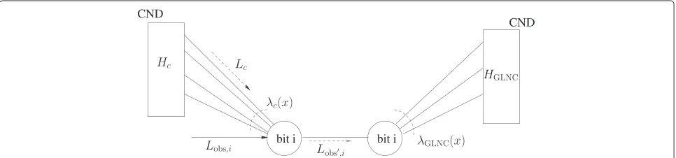
A bit node is essentially protected by two codes: a point-to-point code (Hc) and a network code (HGLNC),
which is illustrated on the factor graph [38] representa-tion (a Tanner notarepresenta-tion [39] is adopted)h of the decoder (Figure 3).
Usually, both codes are characterized by separate degree distributions, denoted as (λc(x),ρc(x)) and
(λGLNC(x),ρGLNC(x))forHcandHGLNC, respectively.
The new lower bound assumes a concatenated decoding scheme. At the destination, first the point-to-point codes
10-6 10-5 10-4 10-3 10-2 10-1 100
7 10 13 16 19 22 25
Outage Probability
Eb/N0 (dB) Conv Outage
Tight Outage
Figure 3The depicted part of the factor graph (using a Tanner notation) illustrates that a bit node (bit i on the figure) is essentially connected to two sets of check nodes, corresponding withHcandHGLNC, respectively.A set of check nodes is denoted as CND for check node decoder. The LLR-value coming from the CND corresponding withHcis denoted asLc. The LLR-value corresponding with the channel observation is denoted asLobs,i.
are decoded and thensoftinformation is passed to the net-work decoder. This is illustrated in Figure 4, where the soft information is denoted by the log-likelihood ratio (LLR) Lobs,i. Note that the bit node of bit i is duplicated to be able to clearly indicateLobs,i. Applying the sum-product algorithm (SPA) on this factor graph or the original factor graph (without node duplication) is equivalent. This fol-lows immediately from the sum-product rule for variable nodes (([40]see Section 4.4)) and ([38], Equation (5)).
The LLRLobs,i can be viewed as anewchannel obser-vation as it remains fixed during the iterative decoding of the network code (HGLNC). The maximum rate that can
be achieved by the network code is given by
1 ms+mr
⎛ ⎝!ms
us=1
I(Sus;Lobs)+
mr
!
ur=1
BurI(Rur;Lobs)
⎞ ⎠.
The terms I(Su;Lobs) and I(Ru;Lobs) are the mutual
informations between the channel inputx ∈ {−1, 1}and the associated random variableLobs, conditioned on the channel realization αu, determined by applying the for-mula for mutual information [36,37], i.e., I(X;Lobs|αu)
is
1−ELobs|{x=1,αu}
log2
)
1+ pLobs(l|x= −1,αu)
pLobs(l|x=1,αu)
*
,
The density of the random variableLobscan be obtained by means of density evolution [41], given the degree distri-butions of the point-to-point code, or by means of Monte Carlo simulations, given the actual factor graph of the point-to-point code. Both approaches yield to the same results in our simulations.
Similarly to the conventional case, an outage event, denoted asEout,2is given by
Eout,2=
+,
Rn≥
ms
us=1I(Sus;Lobs)+
mr
ur=1BurI(Rur;Lobs)
ms+mr
-∪ms us=1
,
Rn ms ≥
I(Sus;Lobs)+j:us∈T(j)BjI(Rj;Lobs)
ms+mr
-.
.
Note that the network coding rate is used instead of the overall rateRc, which corresponds to Proposition 1.
The tight lower bound presented here is a valid lower bound if the point-to-point codes are first decoded, fol-lowed by the network code, without iterating back to the point-to-point codes.
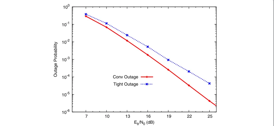
Let us now go back to the small network example with ms=mr=3, considered in the beginning of this section. Figure 2 compares the conventional outage probability (Section ‘Calculation of the outage probability’) with the tighter lower bound proposed here. As mentioned before, the conventional outage probability has a larger diver-sity order than what is achievable, while the tighter lower bound only achieves a diversity order of two.
We are seeing a 3 dB difference at an outage probabil-ity of 10−4. To assess the performance of the network code only, given a certain point-to-point code, the WER of the SMARC-JNCC should be compared with the tight
lower bound presented here. In the subsequent sections, we always include both lower bounds.
7 Numerical results
In this section, we provide numerical results for the SMARC-JNCC. We will clarify the proposed techniques on an illustrating network example, wherems = mr = 5 (Figure 5). We use the same network example as in [17,18] so that a comparison is possible.
For simplicity, we assume non-reciprocal interuser channel in the simulation results. Note that in the case that ms > 4 and Algorithm 1 is used to construct
{T(ur),ur = 1,. . .,mr}, reciprocity is irrelevant for our proposed code, as it applies thati∈/T(j)ifj∈T(i).
We compare the error rate performance of the SMARC-JNCC with the outage probability limit and the tighter lower bound, which are presented in Section ‘Lower bound for the WER’, and with standard network coding techniques (using identity matrices inHGLNC) and a
lay-ered network construction (also using identity matrices in HGLNC, and where, at the destination, the network code is
only decoded after decoding all point-to-point codewords separately and taking a hard decision).
The point-to-point code used in the simulations is an irregular LDPC code [41] characterized by the standard polynomialsλ(x)andρ(x)[41]: tions from an edge perspective. The coefficientsλiandρi
1
2
3
4
5
Figure 5The network example that will be used in this
document is illustrated.The solid lines represent interuser channels, the dashed line is the channel to the destination. Only the channels from the perspective of user 1 are shown for clarity, but all other users see equivalent channels.
are the fraction of edges connected to a bit node and check node, respectively, of degreei. The adopted point-to-point code is fetched from [42], has coding rateRc,p= 6/7 and conforms the following degree distributions:
λ2=0.173, λ3=0.223, λ4=0.095, λ5=0.51
ρ24=0.96, ρ25=0.04.
7.1 Perfect source-relay links
We start by assessing the performance of HGLNC, the
bottom part of Equation (20), which determines the diver-sity order. Therefore, we assume perfect links between sources and relays. Hence, the channel model is the same as described in Section ‘System model’, with the exception of the interuser channels, which are assumed to be per-fect (no fading and no noise). The parameters used for the simulation are K = L = 900, ms = mr = 5 (so that N = 10K = 9000), where N is the block length of the overall codeword. The overall spectral efficiency is R=0.5 bpcu, so thatEb/N0=2γ.
Figure 6 shows that a diversity order of 3 is achieved for SMARC-JNCC, which corroborates Corollary 3. It per-forms at 2.5 dB from the outage probability (because no point-to-point codes are considered, only the con-ventional outage probability is shown), which may be improved by optimizing the degree distributions. We also show a JNCC, where all submatrices Hur, H
ur
us, ∀ur,us are replaced by identity matrices, denoted as the I-JNCC. Finally, we show an I-JNCC with irregular {nur}, with coding matrixM, given by
M=
It is clear that, even without optimizing the SMARC-JNCC, there is a benefit in terms of coding gain compared to the I-JNCC.
7.2 Rayleigh faded source-relay links
10-4 10-3 10-2 10-1 100
7 10 13 16 19 22
Word Error Rate
Eb/N0 (dB) 5.5 dB
2.5 dB Outage
SMARC-JNCC
I-JNCC n=2
I-JNCC irr
Figure 6The word error rate of the SMARC-JNCC is compared to that of the I-JNCC, assuming perfect source-relay channels.
5 (so that N = 10L = 7070). The overall spectral effi-ciency isR = 3/7 bpcu, so thatEb/N0 = 7γ /3. Because
the simulation time would be very large if every point-to-point source-relay link had to be decoded separately, we made an approximation. The word error rate of the point-to-point code when transmitted on a channel with fading gainα is smaller than 10−4whenα2γ = 5.5 dB. Therefore, we assumed that a relay had correctly decoded the source-codeword ifα2γ >5.5 dB and not otherwise.
We also add the performance of the SMARC-JNCC from Section ‘Perfect source-relay links’, corresponding to per-fect source-relay links andR = 0.5 bpcu, as a reference curve (note that the reference curve corresponds to a larger spectral efficiency—the coding rateRc is larger— than for the other curves, which slightly disadvantages the reference curve in terms of error performance).
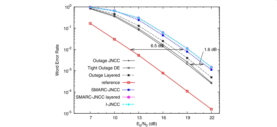
Figure 7 shows that a diversity order of 3 is still achieved, which corroborates Proposition 4. In addition, two main
10-5 10-4 10-3 10-2 10-1 100
7 10 13 16 19 22
Word Error Rate
Eb/N0 (dB) 6.5 dB
1.6 dB
Outage JNCC
Tight Outage DE
Outage Layered
reference
SMARC-JNCC
SMARC-JNCC layered
I-JNCC
Figure 7The word error rate of the SMARC-JNCC is compared to that of the I-JNCC and a layered construction, assuming Rayleigh faded source-relay channels.The reference curve is the performance of the SMARC-JNCC assuming perfect source-relay channels (Section
conclusions can be made. First of all, the coding gain loss due to interuser failures is 6.5 dB, which is very large. Second, the benefit in terms of coding gain of the SMARC-JNCC compared to the I-SMARC-JNCC is considerably decreased, compared to Section ‘Perfect source-relay links’, which corresponds to the small horizontal SNR-gap between the outage probabilities of a layered and joint construction. Also note that the tighter lower bound using density evo-lution, is close to the conventional lower bound in this case (probably due to the larger coding rateRc,p). Finally, the WER performance of a layered construction is shown, which coincides with that of the I-JNCC.
7.3 Gaussian source-relay links
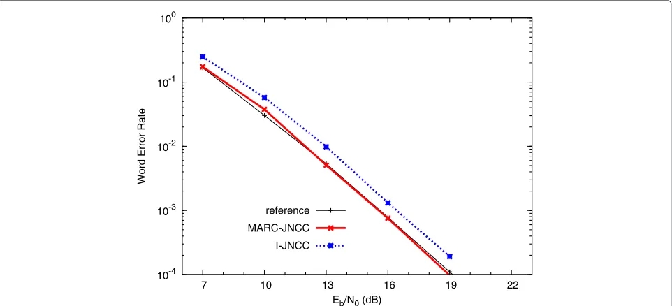
We test again the complete parity-check matrixHof the SMARC-JNCC, now assuming that the source-relay links are Gaussian, having additive white Gaussian noise only, without fading; fading occurs on the source-destination and relay-destination links only. We assume that the aver-age SNR is the same for all channels. The parameters used for the simulation are the same as in Section ‘Rayleigh faded source-relay links’.
Figure 8 shows that in the case of Gaussian interuser channels, the loss compared to perfect interuser chan-nels is very small. Furthermore, the performance of the I-JNCC has improved a lot in comparison with Section ‘Perfect source-relay links’, where HGLNC only was used.
The degree distributions causing the poor coding gain of the I-JNCC in Section ‘Perfect source-relay links’, have changed considerably through the point-to-point codes, significantly improving the coding gain.
8 Conclusion
We put forward a general form of joint network-channel codes (JNCCs) for a wireless communication network where sources also act as relay. The influence of important parameters of the JNCC on the diversity order is studied and an upper and lower bound on the diversity order are proposed. The lower bound is only valid for the case where the number of sources is equal to the number of relays, and where each relay only helps two sources.
We then proposed a practical JNCC that is scalable to large networks. Using the diversity analysis, we managed to rigorously prove its achieved diversity order, which is optimal in a well identified set of wireless networks. We verified the performance of a regular LDPC code via numerical simulations, which suggest that as networks grow, it is difficult to perform significantly better than a standard layered construction.
Appendix 1
Proof of Proposition 1
The maximal diversity order can be derived using the diversity equivalence between a block BEC and a BF chan-nel [24,25]. Assume a block BEC, so that a blocksusorrur is completely erased or perfectly known. Consider the case thate1blocks of length 2Lande2blocks of lengthLhave
been erased, wheree=e1+e2is the total number of
era-sures,e1≤ msande2≤ mr−ms. Hence, the number of unknown bits is equal toe12L+e2L. Considering the
struc-ture ofH from (6) containing the block-diagonal matrix Hc, it follows that thee12L+e2Lerased bits appear in only
(2e1+e2)(L−K)+mrKof the available(ms+mr)L−msK
10-4 10-3 10-2 10-1 100
7 10 13 16 19 22
Word Error Rate
Eb/N0 (dB) reference
MARC-JNCC
I-JNCC
parity equations, i.e.,(2e1+e2)(L−K)equations
involv-ing Hc and allmrK equations involvingHGLNC. Hence,
the unknown bits can be retrieved only if there are suf-ficient linearly independent useful equations. This yields the necessary condition:
mr ≥2e1+e2. (23)
Denoting by e = e1+ e2 the total number of erased
blocks, the largest valueemaxofefor whiche1ande2
sat-isfy (23) for alle1 ≤ ms ande2 ≤ mr −ms is given by
emax=
⎧ ⎨ ⎩
mr
2
mr ≤2ms
mr−ms mr>2ms
(24)
Hence,dmax=emax+1, yielding Proposition 1.
Appendix 2
Proof of Proposition 3
Before we present the actual proof, we first propose two lemmas.
Lemma 4.Any binary a×b matrix S, a≥ b, where all rows have weight 2 cannot have full rank b.
Proof.If a matrix has full rank, there is no vectorz=0 such thatSz = 0. However, ifShas row weight 2, then S1=0, where1corresponds to a column vector with each entry equal to 1.
Consider now a column vector ofbunknown variables zand a set of constraints on these variables, which are stacked inSso thatSz=c, wherecis a column vector of known constants. In general, solvingSforzcorresponds to performing Gaussian elimination ofS. However, under some conditions, this simplifies to backward substitution.
Lemma 5.If a binary a×b matrix S, a ≥ b, has full rank b and maximal row weight of 2, Gaussian elimination simplifies to backward substitution.
Proof.Without loss of generality, we eliminate all redun-dant (linearly dependent) rows in S to obtain a square matrix of sizeb. By Lemma 4, there must be at least one row inSwith unit weight to have full rank. Starting from this known variable, we can solve for a further variable in zat each step as the row weight is smaller than or equal to 2.
Assume that this backward substitution procedure can-not be continued until all variables are known. That is, after successive decoding, there arek rows consisting of a combination ofzik +zjk where neitherzik nor zjk are known. We split the matrixSinto two parts:Sunknown ∈ {0, 1}k×ms andS
known ∈ {0, 1}ms−k×ms. The former
com-prises the rows involving only unknown variables (note
that the weight of each row of Sunknown is 2). The
lat-ter consists of the rows involving only known variables. If the number of unknown variables is equal tok, then the rank ofSunknownmust be equal tokwhich is
impossi-ble by Lemma 4. So, the matrixSwas not full rank which contradicts our assumption. If the number of unknown variables is smaller thank, then there were redundant (lin-early dependent) rows in Sknown which contradicts the
assumptions again. We conclude that the procedure only fails ifSdoes not have full rank.
To prove Proposition 3, we use the diversity equivalence between a block BEC and the BF channel. In a block BEC, the channel Equation (4) simplifies to
yus =uss
us, us=1,. . .,ms yms+ur =urrur, ur =1,. . .,mr,
(25)
where i = 0 when the channel is erased and i = 1 otherwise. Hence,i=0 ifi∈Eandi=1 ifi∈ ¯E, where
¯
Eis the complement ofE.
Source-codewordssi can be retrieved from the trans-missions in the source phase if i = 0. Decoding the other source-codewords at the destination is performed through the parity-check matrixH(Equation (6)). We split Hin two parts:
H=Hleft Hright
, (26)
where Hleft and Hright have msL and mrL columns, respectively. We also define s =[sT1 . . .sTms]T and r = [rT1 . . .rTmr]T. AsHx=0, we have that
Hlefts=Hrightr. (27)
As we consider a block BEC, some transmissions are perfect. As in Appendix 1, consider the case thate1blocks
of length 2Lande2blocks of lengthLhave been erased,
wheree = e1+e2= |E|is the total number of erasures,
e1 ≤ msande2 ≤ mr −ms. Considering the structure of H from (6) containing the block-diagonal matrix Hc, it follows that thee12L+e2Lerased bits appear in only
(2e1+e2)(L−K)+mrKof the available(ms+mr)L−msK
parity equations, i.e.,(2e1+e2)(L−K)equations
involv-ing Hc and all mrK equations involving HGLNC. Next,
(e1+e2)Kfrom themrKequations involvingHGLNC
can-not be used to solve erased bits ins as these equations always have at least two unknowns. The overall set of equations to decodesthus becomes
⎧ ⎪ ⎪ ⎨ ⎪ ⎪ ⎩
sus=yus ∀us∈ ¯E
Hpyus =0 ∀us∈E
us∈T(ur)H ur
ussus =Hury