R E S E A R C H
Open Access
Stability and convergence of the
Crank-Nicolson scheme for a class of
variable-coefficient tempered fractional
diffusion equations
Wei Qu
1,2and Yong Liang
1**Correspondence:
1State Key Laboratory of Quality
Research in Chinese Medicines & Faculty of Information Technology, Macau University of Science and Technology, Avenida Wai Long, Taipa, Macau, 999078, China Full list of author information is available at the end of the article
Abstract
A Crank-Nicolson scheme catering to solving initial-boundary value problems of a class of variable-coefficient tempered fractional diffusion equations is proposed. It is shown through theoretical analysis that the scheme is unconditionally stable and the convergence rate with respect to the space and time step isO(h2+
τ
2) under a certain condition. Numerical experiments are provided to verify the effectiveness and accuracy of the scheme.MSC: 26A33; 65L12; 65L20; 65N15
Keywords: Crank-Nicolson scheme; tempered fractional diffusion equations; unconditionally stable; convergence; variable coefficients
1 Introduction
This paper is concerned with numerical methods for solving the following initial-boundary value problem of tempered fractional diffusion equations (tempered-FDEs):
∂u(x,t)
∂t =d(x)
κaDαx,λ+κxDαb,λ
u(x,t) +f(x,t),
u(a,t) = , u(b,t) = , t∈[,T],
u(x, ) =u(x), x∈[a,b],
()
wheref(x,t) is the source term,d(x)≥ is the diffusion coefficient functions, the param-etersκ≥,κ ≥ are skewed parameters that control the bias of the dispersion, see
Benson et al. [], andλis non-negative. Here, theaDαx,λu(x,t) andxDαb,λu(x,t) represent
the left and right Riemann-Liouville tempered fractional derivatives of the functionu(x,t) with orderα( <α< ), respectively, defined by (see Baeumera and Meerschaert [])
aDαx,λu(x) =aDαx,λu(x) –αλ
α–∂
xu(x) –λαu(x)
and
xDαb,λu(x) =xDαb,λu(x) +αλ
α–∂
xu(x) –λαu(x),
where
aDαx,λu(x) =e–
λx aDαx
eλxu(x)= e
–λx
(n–α)
∂n ∂xn
x
a
eλξu(ξ)
(x–ξ)α–n+dξ
and
xDαb,λu(x) =e
λx xDαb
e–λxu(x)= (–)
neλx
(n–α)
∂n ∂xn
b
x
e–λξu(ξ)
(ξ–x)α–n+dξ,
where(·) denotes the gamma function, and∂xis the first order partial differential
opera-tor with respect tox. Truly, whenλ= , it reduces to theαth order left and right Riemann-Liouville fractional derivatives ofu(x), respectively, then the above equation () reduces to fractional diffusion equations (FDEs).
From the existing literature, tempered-FDEs () is an exponentially-tempered extension of FDEs, which has proven to be an excellent tool in capturing some rare or extreme events in geophysics [–] and finance [, ]. For the FDEs problems, there are a variety of nu-merical schemes, and their fast algorithms developed extensively in the past decades. We refer readers to [–] and the references therein for the recent progress in these prob-lems. In recent years, Deng’s group have further derived some high order difference ap-proximations for the left and right Riemann-Liouville tempered fractional derivatives in [], and their results have been an interest in the numerical simulation of the tempered fractional Black-Scholes equation for European double barrier option []. Moreover, the tempered fractional diffusion models are also used to simulate exponential tempering of the power-law jump length of the continuous time random walk and the Fokker-Planck equation of the new stochastic process, see [, ]. However, in these cases, the diffusion coefficients are usually constants, few papers have focused on the tempered fractional dif-fusion model with variable coefficients. Therefore, it is the aim of this paper to derive a class of variable-coefficient tempered fractional diffusion models.
The paper is organized as follows. In Section , we apply the Crank-Nicolson discretiza-tion for the tempered-FDEs, and the desired order in space and time is obtained. In Sec-tion , it is shown that the method is uncondiSec-tionally stable and convergent. Numerical examples are presented in Section to verify our theoretical analysis. Finally, Section presents the conclusion.
2 The Crank-Nicolson discretization for the tempered fractional diffusion equations
To develop the Crank-Nicolson scheme for problem (), we leth=Nb–+a andτ=MT be the space step and time step respectively, whereN,Mare some given positive integers. Then the spatial and temporal partitions can be defined byxi=a+ih, i= , , . . . ,N+ and
tm=mτ,m= , , . . . ,M. Next, for convenience, we introduce the following notation:
tm+ =
(tm+tm+), f
m+
Note that Li and Deng [] have established a second order tempered-WSGD operators
aDαx,λandxDαb,λto approximate the left and right Riemann-Liouville tempered fractional
derivatives ofu(x) at pointxi, respectively, which gives
aDαx,λu(xi) –αλαu(xi) =aDαx,λu(xi) +O
satisfy the linear system
⎧
Note that there are infinite many solutions of linear system (). However, the rank the coefficient matrix is so that a solution can be uniquely determined when one ofγiis
provided. They can be collected by the following three sets:
Sα
Our main contributions to this paper are to derive a Crank-Nicolson scheme for a class of variable-coefficient tempered-FDEs and to illustrate the stability and convergence of this scheme.
Let umi ≈u(xi,tm), we can therefore consider the Crank-Nicolson technique to the
tempered-FDEs () with the tempered-WSGD approximations to the tempered fractional derivatives and the second order central difference approximation to∂u
∂x, see [, ]. Then,
neglecting the truncation errors, we derive the following second order finite difference scheme:
form, it is given as
(I–A)um+= (I+A)um+τfm, ()
Toeplitz matrix defined as
gi,j=
3 Stability and convergence of the Crank-Nicolson finite difference scheme
To show the unconditional stability and convergence of the Crank-Nicolson finite differ-ence scheme (), the following results given in [, –] are required.
. (α–)((αα++αα+)+)+<γ<min{(α–)(α
+α+)+
(α+α+) ,
(α–)(α+α+)+ (α+α+) };or
. max{(–αα)(+αα++α–),(–
α)(α+α)
(α+α+)}<γ<(–α)(α
+α–)
(α+α+) ,
we have
g(α)< , g(α)+g(α)> , gk(α)> , ∀k≥,
and
∞
k=
gk(α)=γehλ+γ+γe–hλ –e–hλα.
Lemma (Quarteroni et al. []) If A∈Cn×n,let H=A+A∗
be the hermitian part of A, then for any eigenvalueλof A,the real partRe(λ(A)) < satisfies
λmin(H)≤Reλ(A)≤λmax(H),
whereλmin(H)andλmax(H)are the minimum and maximum of the eigenvalues of H, re-spectively.
Lemma (Quarteroni et al. []) A real matrix A of order N is negative definite if and
only if its symmetric part H=A+A∗is negative definite;H is negative definite if and only if the eigenvalues of H are negative.
Definition The numerical range of matrixAis defined as
W(A)≡v∗Av:v∈Cn,v∗v= .
Lemma (Horn and Johnson []) Let A,B∈Cn×n,if B is positive definite,thenσ(AB)⊂
W(A)W(B),whereσ(AB)is the spectrum of AB.
Lemma (Quarteroni and Valli []; Discrete Gronwall’s inequality) Assume that{kn}
and{pn}are non-negative sequences,and the sequence{φn}satisfies
φ≤c, φn≤c+ n–
l= pl+
n–
l=
klφl, n≥,
where c≥.Then the sequence{φn}satisfies
φn≤
c+
n–
l= pl
exp
n–
l= kl
, n≥.
Next, we analyze the stability of finite difference scheme (), we have the following the-orem.
Proof LetM:=εκG+εκGT+η(κ
–κ)W, thenA=DM, note that
M+MT
=ε
(κ+κ)
G+GT+η(κ–κ)
W+WT
=ε(κ+κ)
G+GT.
From [], we note that the matrixGis negative definite. Sinceκ≥,κ≥ andε≥,
then we haveM+M T is also negative definite. Thanks to Lemma , the matrixMis nega-tive definite. Denote byμ(A) an eigenvalue ofA=DM. SinceDis non-negative, combin-ing the negative definite properties ofMand Lemma , we obtain that
σ(A) =σ(DM)⊆W(D)W(M)⊆δ∈C|Re(δ) < .
HenceRe(μ(A)) < , which implies that the inequality
+μ(A) –μ(A)
≤
holds for anyα∈(, ). Therefore, the numerical scheme () is unconditionally stable. In the sequel, we consider the convergence of the numerical scheme (). Let
Vh=
v|v= (v,v,v, . . . ,vN,vN+),v=vN+=
be space grid functions defined on{xi=ih}iN=+. For anyu,v∈Vh, we define
(u,v) =h
N
i= uivi
and the corresponding discreteLnorm
v=(v,v) =
hN
i= vi.
The following theorem describes the convergence of the Crank-Nicolson method when
A=DMis negative definite.
Theorem Let Uimbe the exact solution of tempered-FDEs()and umi be the solution of discrete Eq. ()at mesh point(xi,tm),respectively,where i= , , . . . ,N and m= , , . . . ,M.
For allα∈(, ),if A=DMis negative definite,and the parametersγ,γ,andγsatisfy the hypothesis given in Lemma,we have
Um–um≤Ch+τ, m= , , . . . ,M,
where C is a positive constant,and Um= [Um
Proof Fori= , , . . . ,Nandm= , , , . . . ,M– , the error satisfies the following equation:
Through arrangement, we obtain
Em+–Em–AEm++Em=τρm, E= , m= , , . . . ,M– , ()
Recall that the matrixAis negative definite, then
Sinceρim=O(h+τ), it means thatρm
In this section, two numerical examples are given to show the effectiveness and conver-gence orders of the proposed schemes. In the test, we compute the maximum norm errors between the exact and the numerical solutions at the last time step by
e(h,τ) = max
Example Consider the following two-sided tempered fractional diffusion problem:
∂u(x,t)
Example This example is a modification of Example . We replace the diffusion
Table 1 The maximum errors at timet= 1 and convergence orders in spatial and temporal directions withh=τ=N1+1for Example 1 with differentα, andλ= 1.0, the parameters
γ1= 0.7, 0.75, 0.80, respectively, andγ2andγ3are selected in the setS1α(γ1,γ2,γ3)
α N + 1 γ1= 0.70 γ1= 0.75 γ1= 0.80
e(h,τ) Order e(h,τ) Order e(h,τ) Order
1.2 26 1.6718e–06 - 2.0479e–06 - 2.4267e–06
-27 3.9099e–07 2.10 4.7155e–07 2.12 5.5211e–07 2.14
28 9.4311e–08 2.05 1.1268e–07 2.07 1.3106e–07 2.07
29 2.3150e–08 2.03 2.7526e–08 2.03 3.1903e–08 2.04
210 5.7343e–09 2.01 6.8018e–09 2.02 7.8694e–09 2.02
1.5 26 6.3777e–07 - 8.4512e–07 - 1.0529e–06
-27 1.5554e–07 2.04 2.1700e–07 1.96 2.7849e–07 1.92
28 3.8376e–08 2.02 5.4938e–08 1.98 7.1505e–08 1.96
29 9.5342e–09 2.01 1.3826e–08 1.99 1.8118e–08 1.98
210 2.3761e–09 2.00 3.4680e–09 2.00 4.5598e–09 1.99
1.8 26 2.8859e–07 - 9.0103e–08 - 2.0052e–07
-27 9.1854e–08 1.65 3.2151e–08 1.49 3.9194e–08 2.36
28 2.5751e–08 1.83 9.3079e–09 1.79 8.5674e–09 2.19
29 6.7699e–09 1.93 2.4899e–09 1.90 1.9963e–09 2.10
210 1.7328e–09 1.97 6.4317e–10 1.95 4.8152e–10 2.05
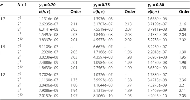
Table 2 The maximum errors at timet= 1 and convergence orders in spatial and temporal directions withh=τ=N1+1for Example 2 with differentα, andλ= 1.0, the parameters
γ1= 0.7, 0.75, 0.80, respectively, andγ2andγ3are selected in the setS1α(γ1,γ2,γ3)
α N + 1 γ1= 0.70 γ1= 0.75 γ1= 0.80
e(h,τ) Order e(h,τ) Order e(h,τ) Order
1.2 26 1.1316e–06 - 1.3936e–06 - 1.6589e–06
-27 2.6235e–07 2.11 3.1707e–07 2.13 3.7199e–07 2.16
28 6.3141e–08 2.05 7.5519e–08 2.07 8.7911e–08 2.08
29 1.5497e–08 2.03 1.8440e–08 2.03 2.1384e–08 2.04
210 3.8397e–09 2.01 4.5577e–09 2.02 5.2758e–09 2.02
1.5 26 5.1105e–07 - 6.6675e–07 - 8.2269e–07
-27 1.2320e–07 2.05 1.7168e–07 1.96 2.2018e–07 1.90
28 3.0239e–08 2.03 4.3597e–08 1.98 5.6957e–08 1.95
29 7.4888e–09 2.01 1.0984e–08 1.99 1.4480e–08 1.98
210 1.8633e–09 2.01 2.7567e–09 1.99 3.6502e–09 1.99
1.8 26 3.7024e–07 - 1.0326e–07 - 1.7880e–07
-27 1.1190e–07 1.73 3.9593e–08 1.38 3.4713e–08 2.36
28 3.0406e–08 1.88 1.1644e–08 1.77 7.5275e–09 2.21
29 7.9086e–09 1.94 3.1315e–09 1.89 1.7469e–09 2.11
210 2.0157e–09 1.97 8.1060e–10 1.95 4.2045e–10 2.05
Other data are the same as those in Example .
From Tables and , we can observe the second order convergence rate in both spatial and temporal directions for differentαinL∞norm, which is consistent with our
theoreti-cal analysis. It is remarked that we numeritheoreti-cally test the eigenvalues of matrixDM+MTD
in Examples and , respectively. We find that all eigenvalues of the matrixDM+MTD
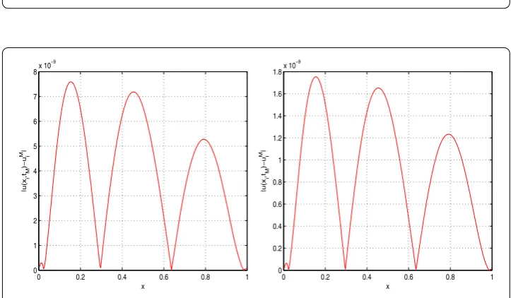
Figure 1 The error curve figures withh=τ=2561 (left) andh=τ=5121 (right) attM= 1 whenα= 1.5, γ1= 0.8 andλ= 1.0 for Example 1.
Figure 2 The error curve figures withh=τ=2561 (left) andh=τ=5121 (right) attM= 1 whenα= 1.8, γ1= 0.8 andλ= 1.0 for Example 2.
In Figures and , we plot the curve figures of the approximating errors (|u(xi,tM) –uMi |)
with different mesh sizes at the final time steptM= via a time-marching procedure, where
γ= . andλ= . whenα= . for Example andα= . for Example , respectively. These figures show that the maximum norm error, defined in Eq. (), becomes relatively smaller as the mesh size becomes smaller, which provides the validation of our results once again.
5 Conclusion
In this paper, the Crank-Nicolson method is proposed for solving a class of variable-coefficient tempered-FDEs (). The method is proven to be unconditionally stable and convergent under a certain condition with rateO(h+τ). Numerical examples show good
Competing interests
The authors declare that they have no competing interests.
Authors’ contributions
All authors read and approved the final manuscript.
Author details
1State Key Laboratory of Quality Research in Chinese Medicines & Faculty of Information Technology, Macau University of
Science and Technology, Avenida Wai Long, Taipa, Macau, 999078, China. 2School of Mathematics and Statistics,
Shaoguan University, Shaoguan, 512005, China.
Acknowledgements
We would like to thank the anonymous reviewers for providing us with constructive comments and suggestions. This work is supported by the Macau Science and Technology Development Funds (Grant No. 099/2013/A3) from the Macau Special Administrative Region of the People’s Republic of China, the National Natural Science Foundation of China under Grant (No. 11601340), and the Natural Science Foundation of Shaoguan University under Grant (No. SY2014KJ07).
Publisher’s Note
Springer Nature remains neutral with regard to jurisdictional claims in published maps and institutional affiliations.
Received: 4 December 2016 Accepted: 21 March 2017
References
1. Benson, DA, Wheatcraft, SW, Meerschaert, MM: The fractional-order governing equation of Lévy motion. Water Resour. Res.36, 1413-1423 (2000)
2. Baeumera, B, Meerschaert, MM: Tempered stable Lévy motion and transient super-diffusion. J. Comput. Appl. Math. 233, 2438-2448 (2010)
3. Meerschaert, MM, Zhang, Y, Baeumer, B: Tempered anomalous diffusions in heterogeneous systems. Geophys. Res. Lett.35, L17403-L17407 (2008)
4. Metzler, R, Klafter, J: The restaurant at the end of the random walk: recent developments in the description of anomalous transport by fractional dynamics. J. Phys. A37, R161-R208 (2004)
5. Carr, P, Geman, H, Madan, DB, Yor, M: Stochastic volatility for Lévy processes. Math. Finance13, 345-382 (2003) 6. Wang, WF, Chen, X, Ding, D, Lei, SL: Circulant preconditioning technique for barrier options pricing under fractional
diffusion models. Int. J. Comput. Math.92, 2596-2614 (2015)
7. Meerschaert, MM, Tadjeran, C: Finite difference approximations for fractional advection-dispersion flow equations. J. Comput. Appl. Math.172, 65-77 (2004)
8. Sousa, E, Li, C: A weighted finite difference method for the fractional diffusion equation based on the Riemann-Liouville derivative. Appl. Numer. Math.90, 22-37 (2015)
9. Pang, HK, Sun, HW: Multigrid method for fractional diffusion equations. J. Comput. Phys.231, 693-703 (2012) 10. Pan, JY, Ke, RH, Ng, MK, Sun, HW: Preconditioning techniques for diagonal-times-Toeplitz matrices in fractional
diffusion equations. SIAM J. Sci. Comput.36, A2698-A2719 (2014)
11. Lei, SL, Sun, HW: A circulant preconditioner for fractional diffusion equations. J. Comput. Phys.242, 715-725 (2013) 12. Qu, W, Lei, SL, Vong, SW: Circulant and skew-circulant splitting iteration for fractional advection-diffusion equations.
Int. J. Comput. Math.91, 2232-2242 (2014)
13. Wang, H, Basu, TS: A fast finite difference method for two-dimensional space-fractional diffusion equations. SIAM J. Sci. Comput.34, A2444-A2458 (2012)
14. Lin, FR, Yang, SW, Jin, XQ: Preconditioned iterative methods for fractional diffusion equation. J. Comput. Phys.256, 109-117 (2014)
15. Chen, MH, Deng, WH: Fourth order accurate scheme for the space fractional diffusion equations. SIAM J. Numer. Anal. 52(3), 1418-1438 (2014)
16. Tian, WY, Zhou, H, Deng, WH: A class of second order difference approximations for solving space fractional diffusion equations. Math. Comput.84, 1703-1727 (2015)
17. Li, C, Deng, WH: High order schemes for the tempered fractional diffusion equations. Adv. Comput. Math.42, 543-572 (2016)
18. Zhang, H, Liu, FW, Turner, I, Chen, S: The numerical simulation of the tempered fractional Black-Scholes equation for European double barrier option. Appl. Math. Model.40, 5819-5834 (2016)
19. Zheng, M, Karniadakis, GE: Numerical methods for SPDEs with tempered stable processes. SIAM J. Sci. Comput.37, A1197-A1217 (2015)
20. Chakrabarty, Á, Meerschaert, MM: Tempered stable laws as random walk limits. Stat. Probab. Lett.81, 989-997 (2011) 21. Sabzikar, F, Meerschaert, MM, Chen, J: Tempered fractional calculus. J. Comput. Phys.293, 14-28 (2015)