Lucas polynomials semi analytic solution for fractional multi term initial value problems

(1)

R E S E A R C H

Open Access

Lucas polynomials semi-analytic solution for

fractional multi-term initial value problems

Mahmoud M. Mokhtar

1*

_{and Amany S. Mohamed}

2

*_{Correspondence:}

[email protected] 1_{Department of Basic Science,}

Faculty of Engineering, Modern University for Technology and Information (MTI), El-Mokattam, Egypt

Full list of author information is available at the end of the article

Abstract

Herein, we use the generalized Lucas polynomials to ﬁnd an approximate numerical solution for fractional initial value problems (FIVPs). The method depends on the operational matrices for fractional diﬀerentiation and integration of generalized Lucas polynomials in the Caputo sense. We obtain these solutions using tau and collocation methods. We apply these methods by transforming the FIVP into systems of algebraic equations. The convergence and error analyses are discussed in detail. The

applicability and eﬃciency of the method are tested and veriﬁed through numerical examples.

MSC: 65M70; 11B39; 34A08; 41A25

Keywords: Caputo derivative; Fractional diﬀerential equations; Spectral methods; Generalized Lucas polynomials

1 Introduction

Ordinary and partial derivatives are special cases of fractional order derivatives. Many scientists are interested in linear and nonlinear fractional differential equations (FDEs). Many phenomena are described using fractional-order differentiation and integration. Their applications appeared in fluid, engineering, mechanics, physics, mathematics, op-tics, and other fields of science. So the fractional calculus investigates the rules, properties of derivatives, and integrals of noninteger orders. For handling these equations, the re-searchers apply many numerical methods such as finite difference method [1–3], finite element method [4–6], homotopy analysis method [7,8], variational iteration method [9– 11], a domain decomposition method [12–15], and Haar wavelet method [16,17].

Recently, the approximate solutions of the fractional differential equations have been evaluated by the spectral methods. These methods help to solve different kinds of dif-ferential equations with small error and a small number of unknowns; [18] solutions of fractional differential equations by using Jacobi operational matrix, [19] solutions of third and fifth-order differential equations by using Petrov–Galerkin methods, [20] solutions of fractional differential equations by using shifted Jacobi spectral approximations. The most used spectral methods are the Galerkin, collocation, and tau methods; [21] solutions of time-fractional telegraph equation by using Legendre–Galerkin algorithm, [22] solution for telegraph equation of space fractional order by using Legendre wavelets spectral tau algorithm, [23] solutions of differential problems by using tau method, [24] solutions for

(2)

the parabolic and elliptic partial equations by the ultra-spherical tau method, [25] solu-tions for a class of variable-order fractional diﬀerential equasolu-tions by using Jacobi wavelets method. The choice of this method depends on the type of the investigated problem and its initial and boundary conditions. For more applications about numerical and exact so-lutions of fractional diﬀerential models, please see [26–37].

Multi-term fractional IVPs appear in many applications in various disciplines, most of numerical studies use the orthogonal polynomials, only rare studies use nonorthogonal polynomials, this motivates us to use these polynomials as a new basis functions, to test their ability to handle these problems.

In this paper, we solve the fractional ordinary diﬀerential equations with initial and boundary conditions applying generalized Lucas polynomials. We obtain the integrated equations and solve them. We use tau and collocation methods to evaluate numerical so-lutions. We have a system of nonlinear algebraic equations with initial and boundary con-ditions. Then we solve them by using Mathematica. We compare our numerical results with the Haar wavelet method [38].

There are many techniques in literature to handle multi-term fractional IVPs using or-thogonal polynomials, i.e., Legendre, Chebyshev, Jacobi, and others, and there are very few studies on nonorthogonal linearly independent set of polynomials, i.e., Lucas and Fi-bonacci polynomials. The main advantages of the present technique is that new polyno-mials can be used as a basis for spectral methods, the generation of these polynopolyno-mials is easy, and the exponential rate of convergence.

The results in this paper are more eﬃcient and of higher accuracy than the other meth-ods. The sections are organized as follows. In section 2 deﬁnitions, properties of fractional calculus, and generalized Lucas polynomials, which are used in the following sections, are introduced. In section 3 derivatives for generalized Lucas polynomials of integer and frac-tional orders are stated. In section 4 the algorithm of this method is explained. In section 5 we investigate the convergence and error analysis. In section 6 we give some examples and their numerical solutions. In the last section we introduce some conclusions.

2 Preliminaries

In this section, some deﬁnitions, properties for fractional calculus [39–41], and the gen-eralized Lucas polynomials [42,43] are stated. We introduce the important relations for the generalized Lucas polynomials which will be used in the following sections.

2.1 Properties and deﬁnitions of fractional calculus

Deﬁnition 1 The fractional integral of orderβ(β≥0) according to Riemann–Liouville is

⎧ ⎨ ⎩

Iβ_g₍_z_{) =} 1

Γ(β) z

0(z–t)

β–1_g₍_t₎_dt_, _β_{> 0,}_z_{> 0,}

I0_g₍_z_{) =}_g₍_z_).

AndIβ_{satisﬁes the following properties:}

⎧ ⎪ ⎪ ⎨ ⎪ ⎪ ⎩

Iβ_Iγ₌_Iβ+γ_,

Iβ_Iγ₌_Iγ_Iβ_,

Iβ_zυ₌ Γ(υ+1)

Γ(υ+β+1)z

(3)

Deﬁnition 2 The fractional derivative of orderβaccording to Caputo

Dβg(z) =Im–βDmg(z) = 1 Γ(m–β)

z

0

(z–t)m–β–1g(m)(t)dt, (1)

wherem– 1 <β≤m, andDβ_{satisﬁes the following properties:}

⎧ ⎨ ⎩

(Dβ_Iβ_g₎₍_z_{) =}_g₍_z_),

Dβ_zυ₌ Γ(υ+1)

Γ(υ–β+1)z

υ–β_. (2)

For more details about the properties of fractional derivatives, please see [43].

2.2 An overview and relations of generalized Lucas polynomials

Lucas polynomialsLj(z) [43] have the following recurrence relation:

Lj+2(z) =zLj+1(z) +Lj(z), (3)

with the initial values

L0(z) = 2, L1(z) =z. (4)

Lucas polynomials have Binet’s form

Lj(z) =

(z+√z2_{+ 4)}j_{+ (}_z_–√_z2_{+ 4)}j

2j , j≥0, (5)

and also have the power form

Lj(z) =j

j

2

i=0

1

j–i j–i

i

zj–2i, j≥1, (6)

where jrepresents the largest integer less than or equal toj. Ifaandb are nonzero real numbers, the sequence of Lucas polynomials{Lj(z)}j≥0is generalized by the sequence

{ϕ_ja,b(z)}j≥0generated by the recurrence relation

ϕ_ja,b(z) =azϕ_ja_–1,b(z) +bϕ_ja_–2,b(z), j≥2, (7)

with the initial values

ϕ₀a,b(z) = 2, ϕ₁a,b(z) =az, (8)

so Lucas polynomialsLj(z) are derived fromϕja,b(z) ifa=b= 1. We have the following:

ϕ₂a,b(z) =az2+ 2b, ϕ₃a,b(z) =a3z3+ 3abz, (9)

(4)

whereϕ_ja,b(z) have the power form

ϕ_ja,b(z) =j j

2

n=0

aj–2n_bnj–n n

j–n z

j–2n_, _j_≥_1, ₍₁₁₎

and

ϕ_ja,b(z) = 2j

j

m=0

ambj–2m_ζ_j₊_kj–n

n

j+m z

m_, _j_≥_1, ₍₁₂₎

where

ζ=

⎧ ⎨ ⎩

1, even,

0, odd. (13)

ϕa_j,b(z) have Binet’s form

ϕ_ja,b(z) =(az+ √

a2_z2_{+ 4}_b₎j_{+ (}_az_–√_a2_z2_{+ 4}_b₎j

2j , j≥0. (14)

The following relations, used for solving the problems, are very important.

3 Integer and fractional derivatives of generalized Lucas vector

In this section, we state the integer and fractional derivatives of generalized Lucas poly-nomials in a matrix form.

3.1 Integer derivatives for generalized Lucas matrix

Suppose that the functionW(z) can be expanded in terms of generalized Lucas polyno-mials

W(z) =

∞

i=0

eiϕia,b(z). (15)

If we approximate this function as

W(z)≈WN(z) = N

i=0

eiϕia,b(z) =ETΦ(z), (16)

where

ET= [e0,e1, . . . ,eN], (17)

Φ(z) =ϕ₀a,b(z),ϕ₁a,b(z), . . . ,ϕa_N,b(z)T. (18)

If the ﬁrst derivative of dΦ_dz(z)is written as

dΦ(z)

dz =H

(5)

whereH(1)_{= (}_H(1)

3.2 Fractional derivatives for generalized Lucas matrix

We state in this section the fractional derivative of generalized Lucas matrix, which is the general case for integer derivative.

Theorem 1 The fractional derivatives of generalized Lucas vector,which is deﬁned in(14),

have the form[42]

have the elements in the form

H_nmβ =

4 The algorithm of the method

In this section, we explain the method for solving the boundary FDE with constant coef-ﬁcients by using generalized Lucas polynomials

(6)

with the boundary conditions

W(i)(0) =ai, i= 0, 1, 2, . . . , (28)

where 0 <α≤1, 1 <β≤2. Suppose that equation (27) has the approximating solution

W(z)≈WN(z) =ETΦ(z). (29)

By using Theorem1, we have

Dβ_W₍_z₎_≈_z–β_ET_H(β)_Φ₍_z_), ₍₃₀₎

and now the residual of equation (27) has the form

R(z) =z–β_ET_H(β)_Φ₍_z_{) +}_z–α_ET_H(α)_Φ₍_z_{) +}_ET_H(2)_Φ₍_z_{) +}_ET_Φ₍_z_{) –}_g₍_z_). ₍₃₁₎

Then we have

zβ_R₍_z_{) =}_ET_H(β)_Φ₍_z_{) +}_zβ–α_ET_H(β)_Φ₍_z_{) +}_zβ_ET_H(2)_Φ₍_z_{) +}_zβ_ET_Φ₍_z_{) –}_zβ_g₍_z_). ₍₃₂₎

By using the tau method, we obtain the system of equations

1

0

zβR(z)ϕ_ia,b(z)dz= 0, i= 0, 1, . . . . (33)

With the boundary conditions (28), we have

ETH(i)Φ(0) =ai, i= 0, 1, 2, . . . . (34)

Equations (33)–(34) give a linear system of equations in coeﬃcients ei,i= 0, 1, . . . ,N.

These coeﬃcients can be eﬃciently solved by Gaussian elimination.

5 Investigation of convergence and error analysis

In this section, we explain the convergence and error analysis of generalized Lucas expan-sion. The following lemmas are satisﬁed.

Lemma 1 For all t∈[0, 1],the following inequality holds for generalized Lucas polynomi-als:

ϕ_ia,b≤2a+√a2₊_bi_. ₍₃₅₎

Proof See Abd-Elhameed and Youssri (2017) [43].

Lemma 2

ϕ_ia,b= 2i

i

k=0

(7)

where

λi,k=

ak_bi–₂k_ζ i+k

i+k

2

i–k

2

i+k . (37)

Theorem 2 If W(z)is deﬁned on[0, 1]and|W(i)₍₀₎_{| ≤}_Li_,_i_≥_0,_{where L is a positive}

con-stant and if W(z)has the expansion

W(z) =

∞

i=0

eiϕia,b(z). (38)

Then one has

|ei| ≤

|a|–i_Li_cosh_(2|_a_|–1_b12_L₎

i! . (39)

IfεN=max|W(z) –WN(z)|, then we have the following truncation error.

Theorem 3 We have the following truncation error estimate:

εN<

2eL(1+√1+a–2_b₎_cosh₍₂_L₍₁₊√₁₊_a–2_b₎₎₍₁₊√₁₊_a–2_b₎N+1

(N+ 1)! (40)

or

εN<

2eLρcosh(2Lρ)ρN+1

(N+ 1)! , (41)

whereρ= 1 +√1 +a–2_b_.

Lemma 3 The derivatives ofϕ_i(α),ϕ_i(β),andϕ_iare denoted by the following estimates:

(i) ϕ_i(α)≤2i3,

(ii) ϕ_i(β)≤2i3,

(iii) ϕ_i≤2i3.

Proof By applying the diﬀerential operators to the right-hand side of equation (29) and noting thatt< 1, and ﬁnally by induction oni, we get the desired results.

Theorem 4 If W(z) =∞_i₌₀eiϕai,b(z)is the exact solution of equation(21)satisﬁes the

hy-potheses of Eq. (6)and W(z)is approximated by WN(z) =

N

i=0eiϕia,b(z),then we have the

following global error estimate:

N=WN+W

(α)

N +W

(β)

N +WN–g<

ΩNξ

(8)

whereΩis a generic constant and

ξ= 3A+ 1, A= L

|a|. (43)

Proof Now the global error estimate

N=WN+W

From equation (21) we have

N=WN–W+W

series comparison test, we have

∞

In this section, we solve some examples on equations (21), (22) using the generalized Lucas polynomials.

Example1 Consider the following fractional-order initial value problem [38]:

DβW(z) + 3

57W(z) =z+

3zβ+1

(9)

We apply the generalized Lucas tau method and obtain the following equations:

2

We solve these equations by Mathematica, we obtain

(10)

Table 1 Maximum absolute errorsEof Example1

z m= 32

β= 1.4

N= 16

β= 1.4

m= 32

β= 1.6

N= 16

β= 1.6

m= 32

β= 1.8

N= 16

β= 1.8

m= 32

β= 2

N= 16

β= 2

0.1 1.4·10–6 1.9·10–7 1.5·10–7 6.9·10–8 1.4·10–7 1.6·10–8 3.5·10–8 5.5·10–18 0.2 6.9·10–9 7.2.0·10–7 3.8·10–8 7.3·10–8 8.9·10–7 1.7·10–8 6.5·10–8 2.6·10–19 0.3 3.3·10–8 6.02·10–7 5.7·10–7 6.0·10–8 1.1·10–7 1.3·10–8 8.7·10–8 6.0·10–18 0.4 3.1·10–7 9.6·10–8 3.8·10–7 3.4·10–8 1.8·10–7 7.7·10–9 9.7·10–8 2.0·10–18 0.5 7.8_·10–7 _8.1_·₁₀–10 _3.6_·₁₀–7 _2.8_·₁₀–10 _2.6_·₁₀–7 _6.6_·₁₀–11 _8.9_·₁₀–8 _1.1_·₁₀–17 0.6 1.5·10–6 _9.6_·₁₀–8 _2.3_·₁₀–7 _2.8_·₁₀–8 _6.0_·₁₀–7 _5.6_·₁₀–9 _5.9_·₁₀–8 _4.1_·₁₀–18 0.7 4.8·10–7 _1.1_·₁₀–7 _3.6_·₁₀–8 _3.3_·₁₀–8 _1.0_·₁₀–6 _6.7_·₁₀–9 _4.8_·₁₀–9 _5.5_·₁₀–18 0.8 7.9·10–7 _1.1_·₁₀–7 _2.2_·₁₀–7 _2.9_·₁₀–8 _1.8_·₁₀–7 _5.3_·₁₀–9 _8.0_·₁₀–8 _6.1_·₁₀–17 0.9 1.1·10–6 _6.5_·₁₀–8 _5.5_·₁₀–7 _1.5_·₁₀–8 _3.5_·₁₀–7 _2.6_·₁₀–9 _1.9_·₁₀–7 _2.2_·₁₀–17

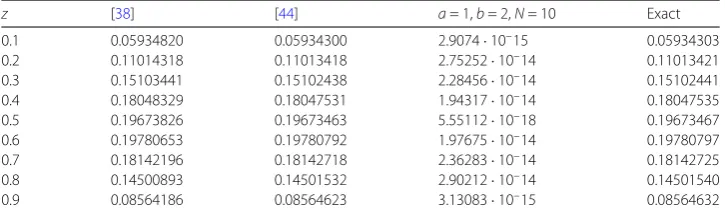
Table 2 Comparison between diﬀerent errorsEof Example2

z [38] [44] a= 1,b= 2,N= 10 Exact

0.1 0.05934820 0.05934300 2.9074·10–15 0.05934303

0.2 0.11014318 0.11013418 2.75252·10–14 0.11013421

0.3 0.15103441 0.15102438 2.28456·10–14 0.15102441

0.4 0.18048329 0.18047531 1.94317·10–14 0.18047535

0.5 0.19673826 0.19673463 5.55112_·10–₁₈ _0.19673467

0.6 0.19780653 0.19780792 1.97675·10–₁₄ _0.19780797

0.7 0.18142196 0.18142718 2.36283·10–₁₄ _0.18142725

0.8 0.14500893 0.14501532 2.90212·10–₁₄ _0.14501540

0.9 0.08564186 0.08564623 3.13083·10–₁₅ _0.08564632

e2=

33(–222,794 + 3,871,765√π+ 57,000π) 5a2_{(107,324,217 – 341,088}√_π_{+ 320}_π₎,

e3= –

143(–27,588 – 393,483√π+ 11,400π) 6a3_{(107,324,217 – 341,088}√_π_{+ 320}_π₎.

(57)

In Table1, we compare our results for the casea=b= 1 andN= 16 with the results of [38] form= 32 for diﬀerent values ofβ. In Table2, we compare between diﬀerent solutions of Example2.

DβW(z) –DαW(z) =ez–1+ 1, 0 <β≤1, 1 <α≤2, (58)

W(0) = 0, W(1) = 0. (59)

The exact solution of equation (38) isW(z) =z(1 –ez–1_{). The residual of this equation is}

zβ_R₍_z_{) =}_ET_H(β)_Φ₍_z_{) –}_zβ–α_ET_H(α)_Φ₍_z_{) –}_zβ_ez–1_–_zβ_. ₍₆₀₎

DβW(z) +e

–3π √

πW(z)

= e

–3π

40√π

(11)

W(0) = 0, W(1) = –1

40. (62)

The exact solution of equation (41) isW(z) =z2(z3–37₂₀z+33₄₀). The residual of this equa-tion is

zβR(z) =ETH(β)Φ(z) +e

–3π √

πz

β

ETΦ(z)

– e

–3π

40√π

z240z2– 74z+ 33+ 4e3π√z128z2– 148z+ 33zβ.

We apply our algorithm for the casea= 1,b= 2,N= 5,β=3

2, which yields

e1= 511/10, e3= –237/20, e5= 1,

e0= –33/2, e2= 233/4, e4= 0,

and consequently,

W(z) = –(33/2)2 + (511/10)z+ (233/4)4 +z2– (237/20)6z+z3+ 20z+ 10z3+z5,

which is the exact solution.

W(z) + 8 17D

β

W(z) +13 51W(z) =

z–12 89,250√π

48p(z) + 7√zq(z), 1≤β< 2, (63)

where

p(z) = 16,000z4– 32,480z3+ 21,280z2– 4746z+ 189, (64)

q(z) = 3250z5– 9425z4+ 264,880z3– 44 (65)

W(0) = 0, W(1) = 0. (66)

The exact solution of equation (45) isW(z) =z5_–29z4

10 + 76z3

25 – 339z2

250 + 27z

125. The residual

of this equation is

zβR(z) =zβETH(2)Φ(z) + 8 17E

T_H(β)_Φ₍_z_{) +}13

51z β

ETΦ(z)

– z –1

2+β 89,250√π

(12)

We apply our algorithm for the casea= 2,b= 1,N= 5,β=3₂, which yields

e1= –1439/2000, e3= 179/800, e5= 1/32,

e0= –819/4000, e2= 193/500, e4= –29/160,

and consequently,

W(z) = –(819/4000)2 – (1439/2000)2z+ (193/500)2 + 4z2+ (179/800)6z+ 8z3

– (29/160)2 + 16z2+ 16z4+ (1/32)10z+ 40z3+ 32z5,

which is the exact solution.

7 Conclusion

Herein, a generalized Lucas polynomial sequence approach based on the operational ma-trix of fractional derivatives Lucas polynomials to spectrally solve fractional multi-term initial value problem was successfully applied to handle these equations. Four examples to a system of linear algebraic equations were solved by Mathematica software showing the exponential rate of convergence of the method. This method can be modified in the future work to solve different types of ordinary and partial FDEs with nonhomogeneous conditions and with variable coefficients.

Acknowledgements

The authors are very grateful to the anonymous referees for careful reviewing and crucial comments, which enabled us to improve the manuscript.

Funding

This research received no speciﬁc grant from any funding agency in the public, commercial, or not-for-proﬁt sectors.

Competing interests

The authors declare that they have no competing interests.

Authors’ contributions

All authors contributed equally to this work. All authors read and approved the ﬁnal manuscript.

Author details

1_{Department of Basic Science, Faculty of Engineering, Modern University for Technology and Information (MTI),}

El-Mokattam, Egypt. 2_{Department of Mathematics, Faculty of Science, Helwan University, Helwan, Egypt.}

Publisher’s Note

Springer Nature remains neutral with regard to jurisdictional claims in published maps and institutional aﬃliations.

Received: 20 July 2019 Accepted: 1 November 2019 References

1. Li, C., Zeng, F.: Finite diﬀerence methods for fractional diﬀerential equations. Int. J. Bifurc. Chaos22, 1230014 (2012) 2. Sweilama, N.H., Khader, M.M., Nagy, A.M.: Numerical solution of two-sided space-fractional wave equation using

ﬁnite diﬀerence method. J. Comput. Appl. Math.235, 2832–2841 (2011)

3. Mustapha, K., Furati, K., Knio, O.M., Le Maitre, O.P.: A finite difference method for space fractional differential equations with variable diffusivity coefficient. Mathematics, Numerical Analysis (2018)

4. Badr, A.A.: Finite element method for linear multiterm fractional diﬀerential equations. J. Appl. Math.2012, Article ID 482890 (2012)

5. Jiang, Y., Ma, J.: High-order ﬁnite element methods for time-fractional partial diﬀerential equations. J. Comput. Appl. Math.235, 3285–3290 (2011)

6. Zhu, X., Yuan, Z., Wang, J., Nie, Y., Yang, Z.: Finite element method for time–space-fractional Schrodinger equation. Electron. J. Diﬀer. Equ.2017, 166 (2017)

(13)

8. Jafari, H., Seiﬁ, S.: Solving a system of nonlinear fractional partial diﬀerential equations using homotopy analysis method. Commun. Nonlinear Sci. Numer. Simul.14, 1962–1969 (2009)

9. Sakar, M.G., Erdogan, E., Yildirim, A.: Variational iteration method for the time fractional Fornberg–Whitham equation. Comput. Math. Appl.63, 1382–1388 (2012)

10. Khan, Y., Faraz, N., Yildirim, A., Wu, Q.: Fractional variational iteration method for fractional initial-boundary value problems arising in the application of nonlinear science. Comput. Math. Appl.62, 2273–2278 (2011)

11. Singh, B.K., Kumar, P.: Fractional variational iteration method for solving fractional partial diﬀerential equations with proportional delay. Int. J. Diﬀer. Equ.2017, Article ID 5206380 (2017)

12. Hu, Y., Luo, Y., Lu, Z.: Analytical solution of linear fractional diﬀerential equation by a domain decomposition method. J. Comput. Appl. Math.215, 220–229 (2008)

13. Ray, S.S., Bera, R.K.: Solution of an extraordinary diﬀerential equation by a domain decomposition method. J. Appl. Math.4, 331–338 (2004)

14. Shawagfeh, N.T.: Analytical approximate solutions for nonlinear fractional diﬀerential equations. Appl. Math. Comput.

131, 517–529 (2002)

15. Daftardar-Gejji, V., Jafari, H.: Adomian decomposition: a tool for solving a system of fractional diﬀerential equations. J. Math. Anal. Appl.301, 508–518 (2005)

16. Sweilam, N.H., Nagy, A.M., Mokhtar, M.M.: On the numerical treatment of a coupled nonlinear system of fractional diﬀerential equations. J. Comput. Theor. Nanosci.14, 1184–1189 (2017)

17. Sweilam, N.H., Nagy, A.M., Mokhtar, M.M.: New spectral second kind Chebyshev wavelets scheme for solving systems of integro-diﬀerential equations. Int. J. Appl. Comput. Math.3(2), 333–345 (2017)

18. Doha, E.H., Bhrawy, A.H., Ezz-Eldien, S.S.: A new Jacobi operational matrix: an application for solving fractional diﬀerential equations. Appl. Math. Model.36, 4931–4943 (2012)

19. Abd-Elhameed, W.M., Doha, E.H. Youssri, Y.H.: Efficient spectral Petro–Galerkin methods for third and fifth-order differential equations using general parameters generalized Jacobi polynomials. Quaest. Math.36, 15–38 (2013) 20. Doha, E.H., Bhrawy, A.H., Baleanu, D., Ezz-Eldien, S.S.: On shifted Jacobi spectral approximations for solving fractional

diﬀerential equations. Appl. Math. Comput.219, 8042–8056 (2013)

21. Youssri, Y.H., Abd-Elhameed, W.M.: Numerical spectral Legendre–Galerkin algorithm for solving time fractional telegraph equation. Rom. J. Phys.63, 107 (2018)

22. Mohammed, G.S.: Numerical solution for telegraph equation of space fractional order by using Legendre wavelets spectral tau algorithm. Aust. J. Basic Appl. Sci.10, 381–391 (2016)

23. OrtizE, L., Samara, H.: Numerical solutions of diﬀerential eigen values problems with an operational approach to the tau method. Computing31, 95–103 (1983)

24. Doha, E.H., Abd-Elhameed, W.M.: Accurate spectral solutions for the parabolic and elliptic partial equations by the ultra-spherical tau method. J. Comput. Appl. Math.181, 24–45 (2005)

25. Zaky, M.A., Ameen, I.G., Abdelkawy, M.A.: A new operational matrix based on Jacobi wavelets for a class of variable-order fractional diﬀerential equations. Proc. Rom. Acad., Ser. A: Math. Phys. Tech. Sci. Inf. Sci.18, 315–322 (2017)

26. Baleanu, D., Asad, J.H., Jajarmi, A.: New aspects of the motion of a particle in a circular cavity. Proc. Rom. Acad., Ser. A: Math. Phys. Tech. Sci. Inf. Sci.19(2), 361–367 (2018)

27. Hajipour, M., Jajarmi, A., Baleanu, D., Sun, H.G.: On an accurate discretization of a variable-order fractional reaction–diﬀusion equation. Commun. Nonlinear Sci. Numer. Simul.69, 119–133 (2019)

28. Mohammadi, F., Moradi, L., Baleanu, D., Jajarmi, A.: A hybrid functions numerical scheme for fractional optimal control problems: application to non-analytic dynamical systems. J. Vib. Control24(21), 5030–5043 (2018)

29. Baleanu, D., Jajarmi, A., Asad, J.H.: The fractional model of spring pendulum: new features within diﬀerent kernels. Proc. Rom. Acad., Ser. A: Math. Phys. Tech. Sci. Inf. Sci.19(3), 447–454 (2018)

30. Hajipour, M., Jajarmi, A., Baleanu, D.: On the accurate discretization of a highly nonlinear boundary value problem. Numer. Algorithms79(3), 679–695 (2018)

31. Hajipour, M., Jajarmi, A., Malek, A., Baleanu, D.: Positivity-preserving sixth-order implicit finite difference weighted essentially non-oscillatory scheme for the nonlinear heat equation. Appl. Math. Comput.325, 146–158 (2018) 32. Alsuyuti, M.M., Doha, E.H., Ezz-Eldien, S.S., Bayoumi, B.I., Baleanu, D.: Modified Galerkin algorithm for solving multitype

fractional diﬀerential equations. Math. Methods Appl. Sci.42(5), 1389–1412 (2019)

33. Firoozjaee, M.A., Yousefi, S.A., Jafari, H., Baleanu, D.: On a numerical approach to solve multi-order fractional differential equations with initial/boundary conditions. J. Comput. Nonlinear Dyn.10(6), 061025 (2015) 34. Bhrawy, A.H., Baleanu, D., Assas, L.M.: Efficient generalized Laguerre-spectral methods for solving multi-term

fractional diﬀerential equations on the half line. J. Vib. Control20(7), 973–985 (2014)

35. Rostamy, D., Alipour, M., Jafari, H., Baleanu, D.: Solving multi-term orders fractional diﬀerential equations by operational matrices of BPs with convergence analysis. Rom. Rep. Phys.65(2), 334–349 (2013)

36. Baleanu, D., Shiri, B., Srivastava, H.M., Al Qurashi, M.: A Chebyshev spectral method based on operational matrix for fractional differential equations involving non-singular Mittag-Leffler kernel. Adv. Differ. Equ.2018, 353 (2018) 37. Baleanu, D., Shiri, B.: Collocation methods for fractional differential equations involving non-singular kernel. Chaos

Solitons Fractals116, 136–145 (2018)

38. ur Reham, M., Ali Khan, R.: A numerical method for solving boundary value problems for fractional diﬀerential equations. Appl. Math. Model.36, 894–907 (2012)

39. Miller, K.S., Ross, B.: An Introduction to the Fractional Calculus and Fractional Diﬀerential Equations. Wiley, New York (1993)

40. Podlubny, I.: Fractional Diﬀerential Equations (1999) 41. Rainville, E.D.: Special Functions. Chelsea, New York (1960)

42. Abd-Elhameed, W.M., Youssri, Y.H.: Spectral solutions for fractional diﬀerential equations via a novel Lucas operational matrix of fractional derivatives. Rom. J. Phys.61, 795–813 (2016)

43. Abd-Elhameed, W.M., Youssri, Y.H.: Generalized Lucas polynomials sequence approach for fractional diﬀerential equations. Nonlinear Dyn.89, 1341–1355 (2017)