Simultaneous identification of initial field and spatial heat source for heat conduction process by optimizations

(1)

R E S E A R C H

Open Access

Simultaneous identiﬁcation of initial ﬁeld

and spatial heat source for heat conduction

process by optimizations

Bingxian Wang

1*

_{, Bin Yang}

1

_{and Mei Xu}

1

*_{Correspondence:}

[email protected] 1_{School of Mathematics Science,}

Huaiyin Normal University, Huaian, P.R. China

Abstract

Consider the simultaneous identiﬁcation of the initial ﬁeld and spatial heat source for heat conduction process from extra measurements with the two additional

measurement data at diﬀerent times. The uniqueness and conditional stability for this inverse problem are established by using the properties of a parabolic equation and the representation of solution after reforming the equation. By combining the least squares method with the regularization technique, the inverse problem is

transformed into an optimal control problem. Based on the existence and uniqueness of the minimizer of the cost functional, an alternative iteration process is built to solve this optimizing problem by the variational adjoint method. The negative gradient direction is selected as the first search direction. For further iterations, the alternative iteration algorithm is used for the initial field and heat source identification. The efficiency of the proposed scheme is tested by the numerical simulation experiments.

MSC: 35R30; 35J05; 76Q05

Keywords: Inverse problem; Parabolic equation; Initial ﬁeld; Heat source; Adjoint variational method; Numerics

1 Introduction

Consider the following heat conduction problem:

ut–u=f(x) inΩ×(0,T), (1)

with initial condition

u(x, 0) =φ(x) inΩ, (2)

and boundary condition

u(x,t) = 0 on∂Ω, (3)

whereΩ⊂Rd(d= 1, 2) is bounded,f(x) is the space-dependent heat source andφ(x) is the initial temperature withφ|∂Ω= 0. Iff,φ∈L2(Ω), then the solution of (1) is unique and

(2)

u∈L2_(0,_T_;_H1

0(Ω)) in the distributional sense which satisﬁes (2) (see [1]), and

uL2_(0,T;H1 0(Ω))≤C

fL2₍_Ω₎+φL2₍_Ω₎

,

whereCis independent off andφ.

The problem considered in this paper is to determine the initial temperatureφ(x) and the space-dependent sourcef(x) simultaneously from two additional measurement data at timesT1,T2for 0 <T1<T2≤T:

u(x,T1) =ψ1(x), x∈Ω, (4)

u(x,T2) =ψ2(x), x∈Ω. (5)

It is well known that if the source termf(x) in (1) is given, the recovery of the initial valueφ(x) fromu(x,T) is severely ill-posed. For the classical heat conduction equation, it is called a backward heat conduction problem. Many authors have studied this kind of inverse problem; see [2–7]. On the other hand, when the initial valueφ(x) is known, estimating the sourcef(x) from the final observation is also an ill-posed problem [8,9]. The degree of ill-posedness is equivalent to that of second-order numerical differentiation [10,11]. The problem in this paper was firstly investigated by Johansson and Lesnic in [12] where the uniqueness was presented and an iterative regularization algorithm was used to solve it.

This article is organized as follows. In Sect.2, we give uniqueness analysis and a con-ditional stability result for the inverse problem (1)–(5). An optimization problem is pre-sented and an alternative iteration scheme is constructed by means of the variational ad-joint method in Sect.3. Numerical examples are given in Sect.4.

2 Uniqueness and conditional stability

Supposef(x),φ(x)∈L2(Ω) and setw(x,t) =u(x,t) –φ(x), then (1)–(3) will change into

⎧ ⎪ ⎪ ⎨ ⎪ ⎪ ⎩

wt–w=f(x) –φ(x) inΩ×(0,T),

w(x,t) = 0 on∂Ω,

w(x, 0) = 0 inΩ,

(6)

withw(x,T1) =ψ1(x) –φ(x) andw(x,T2) =ψ2(x) –φ(x). Applying separation of variables, we can obtain the solution to (6) as

w(x,t) =

Ω

t

0

K(t–τ,x,y)f(y) –φ(y)dτdy, (7)

where

K(t–τ,x,y) = ∞

n=1

e–λn(t–τ)_X

n(x)Xn(y).

Thus, fori= 1, 2, we can obtain

Ω

f(y) –φ(y) Ti

0

(3)

Setφ˜(x) =φ(x) withφ(x) = 0 (x∈∂Ω) andψ˜i(x) =ψi(x) (i= 1, 2) withψi(x) = 0 (x∈ mined by means of the measurements at diﬀerent timesT1andT2. So combining with the properties of the problem (1)–(3), we have the following result:

Lemma 2.1 Supposeφ,f ∈L2(Ω),andψ1,ψ2∈H01(Ω),then the solution to the inverse problem(1)–(5)is unique in L2₍_Ω₎_×_L2₍_Ω_).

Now, we give a conditional stability analysis for the inverse problem. Suppose∂Ω∈C2+α

andφ,f ∈C2+α₍_Ω¯_{), then}

ψ1,ψ2∈C2+α(Ω¯)⊂C2(Ω¯)⊂L2(Ω) (13)

by Theorem 2.2.5 in [13].

We divide the time interval [0,T2] into [0,T1] and [T1,T2]. In [T1,T2], for the source f(x), we have the following stability result in the framework of Hölder spaces [14]:

(4)

Now we consider the conditional stability with respect toφin [0,T1] with the aid of the stability result (14). By separation of variables we can obtain the solution to (1)–(4) as follows:

Similarly, from (17), we have

(5)

On the other hand, (18) yields

Now we introduce the following norms ofφandf:

φ2_F1:=

and deﬁne the following admissible set ofφandf:

P1=

From the above analysis, by the linearity of the inverse problem and (14),(24), we have

Theorem 2.2 Suppose∂Ω∈C2+α_._For_φi_∈_P to the inverse problem has the following stability estimate:

(6)

φ1_–_φ22

3 Iteration scheme for solving the optimization problem

We reformulate the inverse problem (1)–(5) as the following optimization problem: Find (φ∗,f∗) such that

Jφ∗,f∗= min

φ∈L2₍_Ω_),f_∈_L2₍_Ω₎J(φ,f), (27) where the cost functional is

J(φ,f) :=J1(φ,f) +J2(φ) +J3(f), (28) ization parameter;φη _and_fη_{are some prior information of}_φ_and_f_{, respectively. Similar}

to a discussion in [15], we have the following result for the optimization problem:

Lemma 3.1 For anyγ > 0,J(φ,f)has a unique pair of minimizers(φ∗,f∗)in L2₍_Ω₎_× L2₍_Ω_).

SettingΩ⊂R2_{, we will propose an alternative iteration scheme for minimizing}_J₍_φ_,_f₎ based on the variational adjoint method to generate the approximate solution to our in-verse problem. The crucial steps are the derivation of the gradient of the cost functional and an eﬃcient iteration scheme based on the gradient.

3.1 Derivation of the gradient of functional

We ﬁrst derive the tangent linear model. Denote byu(x,t),u˜(x,t), andu˘(x,t) the solutions

then by direct calculation foruˆwe have

(7)

Now we calculate the Gatéaux derivative of the cost functionalJ(·,·). Generally, Gatéaux derivative is deﬁned as

(∇fJ,fˆ) + (∇φJ,φˆ) :=lim

So we calculate directly the two limits on the right-hand side of (32), and by means of the conditions of the problem (1)–(3), we have Secondly, deﬁne the adjoint systems:

(8)

Adding (38) to (39), (33) can be changed into

(∇φJ,φˆ) + (∇fJ,fˆ) =

Ω

p1(x, 0)φˆ(x)dx+

T1

0

Ω

p1ˆf dx dt

+

Ω

p2(x, 0)φˆ(x)dx+

T2

0

Ω

p2f dx dtˆ

+γ2

Ω

ˆ

φφ–φηdx+γ2

Ω

ˆ

ff –fηdx.

Due to the irrelevance ofφˆandfˆ, the gradient ofJ(φ,f) at (φ,f) alongφˆ,fˆcan be ob-tained as follows:

∇φJ=p1(x, 0) +p2(x, 0) +γ2

φ–φη, (40)

∇fJ=

T1

0

p1(x,t)dt+

T2

0

p2(x,t)dt+γ2

f –fη. (41)

3.2 Iteration algorithm

Starting from the initial guessφ0(x) andf0(x), we construct the following iteration scheme:

φn+1(x) =φn(x) +r1nD1n, n= 0, 1, 2, . . . , (42)

fn+1(x) =fn(x) +r2nD2n, n= 0, 1, 2, . . . , (43)

whereri

n> 0 (i= 1, 2) is the step size selected by the Wolfe line search [16], andD1n,D2n are the searching directions. The negative gradient direction is selected as the first search direction forD1_n,D2_n. For the succeeding iterations, two kinds of optimization method are used for the initial temperature inversion and the heat source identification, respectively. An alternative iteration scheme is constructed to improve the computation efficiency.

According to the construction of the iterative scheme (42)–(43), we design the following alternate iteration algorithm for solving (φn,fn):

Fix the maximum iterative stepNmax, the error level, and the maximum length of

cor-rection steprmax> 0.

Step 1: Given the initial guessφ0,f0and initial search stepr01,r20∈(0,rmax), calculate

D1₀= –g0:= –∇φJ|(φ0,f0), φ1(x) =φ0(x) +r 1 0D10(x), D2₀= –s0:= –∇fJ|(φ1,f0), f1(x) =f0(x) +r02D20(x).

Repeat forn= 2, 3, 4, . . ..

Step 2: Calculate the two tangent directions ofJwith respect toφ,f:

gn–2=∇φJ|(φn–2,fn–2), gn–1=∇φJ|(φn–1,fn–2), sn–2=∇fJ|(φn–1,fn–2), sn–1=∇fJ|(φn–1,fn–1).

Here, for given(φi,fj), we ﬁrst need to solve the direct problem (1)–(3) and

get the solutionu[φi,fj], and the adjoint problem (34)–(35) is then also solved to

obtainp1[φi,fj],p2[φi,fj], where

(9)

Step 3: Calculate the correction stepξn–1,ζn–1in thenth iteration direction as

ξn–1= gn–1

gn–2, ζn–1=

sT_n–1(sn–1–sn–2) sT

n–2(sn–1–sn–2) .

Step 4: Modify the negative gradient direction and get the new iteration direction ofφn, fn:

D1_n–1= –gn–1+ξn–1D1n–2, D2n–1= –sn–1+ζn–1D2n–2.

Step 5: Calculate the step size(r1_n–1,r_n–12 )for update(φn–1,fn–1)by Wolfe line search. Step 6: Calculate

φn(x) =φn–1(x) +r1n–1D1n–1(x), fn(x) =fn–1(x) +r2n–1D2n–1(x);

Step 7: Check whethermax{gn,sn}<εorn>Nmax? If it is true, stop the iteration

and outputφn,fn. Otherwise, setn+ 1⇒nand return toStep 2.

4 Numerical implementation

In this section, we give two numerical implementations for the iteration algorithm. All the computations were performed using MATLAB 2016a on a personal computer with Intel Core i5 and 8.00 GB memory. Setx= (x1,x2),Ω= [0,π]×[0,π], denote the stepsizes inx1 andx2byh1=π/M1andh2=π/M2, respectively, whereM1,M2∈Nare grid parameters with respect tox1,x2. The stepsize intdenotedτis chosen byT1=N1τ,T2=N2τ. What needs to be explained is that an alternate iterative scheme is proposed. In Example1, we compare the numerical results with the solutions by the primary iteration scheme. The ﬁnal time giving the inversion input data is taken asT1= 1/2,T2= 1 for the two examples, while the noisy ﬁnal measurement data are simulated by

uδ(x,Ti) =u(x,Ti) +δ×randn(x), (44) whererandn(x)∈[–1, 1] are from the normal distribution with mean 0 and standard de-viation 1. Here the direct problem (1)–(3) and adjoint system (34) and (35) are solved by D’Yakonov ADI scheme. The error estimates ofφ(x) andf(x) are deﬁned byL2_-estimation:

errφ_nδ,φ∗=φδ_n–φ∗

L2₍_Ω₎, err

f_nδ,f∗=f_nδ–f∗_L2₍_Ω₎. (45) Example1 The exact solution of (1)–(3) is

u(x1,x2,t) =

2 –e–2tsinx1sinx2, (46)

and thenφ∗(x1,x2) =sinx1sinx2andf∗(x1,x2) = 4sinx1sinx2. According to (46), the noisy data is simulated by

uδ(x1,x2,Ti) =

2 –e–2Ti_sin_x

1sinx2+δ×rand(x1,x2), i= 1, 2. (47)

In this example, we selectφη₌_fη_{= 0 and divide the domain}_Ω_{as 60}_×_{60 pixels and take}

the regularizing parametersγ = 10–2_{. Set}_φ

(10)

in-Figure 1Reconstructions of Example1: (ﬁrst line) exact and approximate solutionsφ(x1,x2) withδ= 0; (second line) approximate solutions forδ= 0.001, 0.01; (third line) approximate solutions forδ= 0.02, 0.03, respectively

put data (47) withδ= 0, 0.001, 0.01, 0.02, 0.03, respectively. The inverse results ofφ(x1,x2) andf(x1,x2) are shown in Figs.1and2. Here, in order to represent the advantage of an alternate iteration in this paper, we also calculateJ(φδ

n,fnδ),err(φnδ,φ∗), anderr(fnδ,f∗) with

δ= 0 by means of alternate iteration and primary iteration, which are shown in Table1. ForJ(φδ

n,fnδ), the functional value is reduced faster than when using alternate iteration af-ter the same number of iaf-terations. Furthermore, the estimated error valueserr(φ_nδ,φ∗) and err(fδ

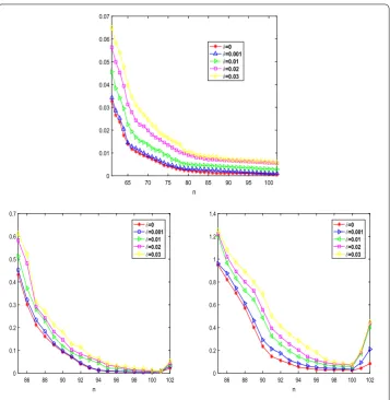
n,f∗) are small after 100 iterations by using the alternate iteration scheme, but respec-tive errors when using the primary iteration scheme are reduced slowly. It can be seen that the eﬃciency of computation is greatly improved by alternate iteration. Figure3(ﬁrst line) shows the numerical performance for noisy input data by giving the behavior ofJ(φδ_n,fδ

(11)

Figure 2Reconstructions of Example1: (ﬁrst line) exact and approximate solutions off(x1,x2) withδ= 0; (second line) approximate solutions forδ= 0.001, 0.01; (third line) approximate solutions forδ= 0.02, 0.03, respectively

Table 1 Functional value ofJ(φ_nδ,f_nδ), errors err(φδ_n,φ∗) and err(f_nδ,f∗) by the primary iteration scheme; “J1”, “err1” represent the results of the alternate iteration scheme

n J(φδ

n,fnδ) J1(φnδ,fnδ) err(φδn,φ∗) err1(φδn,φ∗) err(fnδ,f∗) err1(fnδ,f∗)

85 5.3832E–01 1.5323E–02 1.0866 5.3221E–01 1.4455 1.0483

87 5.2923E–01 1.3229E–02 1.0254 3.1208E–01 1.2833 8.0214E–01

89 5.0202E–01 1.2026E–02 1.0086 1.9327E–01 1.2312 5.0118E–01

91 4.8282E–01 1.1224E–02 9.7452E–01 8.0323E–02 1.1955 2.0543E–01

93 4.6211E–01 1.0981E–02 9.4924E–01 3.8345E–02 1.1523 1.0214E–01

95 4.5886E–01 1.0735E–02 9.3229E–01 1.4148E–02 1.1101 5.1183E–02

97 4.4553E–01 1.0498E–02 9.1223E–01 5.8643E–03 1.0775 2.9752E–02

99 4.2814E–01 8.2701E–03 8.8426E–01 4.8327E–03 1.0291 2.7538E–02

100 4.0755E–01 7.5523E–03 8.7208E–01 4.0462E–03 9.8123E–01 2.5147E–02

(12)

Figure 3Numerical performance ofJ(φδ

n,fnδ) (ﬁrst line), err(φδn,φ∗) (second line, (left)), err(fnδ,f∗) (second line,

(right)) with respect to the number of iterations forδ= 0, 0.001, 0.01, 0.02, and 0.03 of Example1

Example2 The exact initial temperature and the source ﬁeld are

φ(x1,x2) =sin2x1sin2x2, x1,x2∈[0,π],

f(x1,x2) =

⎧ ⎨ ⎩

1, π/4≤x1,x2≤3π/4, 0, else.

Then the exact solution has the same form

u(x1,x2,t) = ∞

n=1 ∞

m=1

Hmn(t)sinmx1sinnx2, 0≤x1,x2≤π, (48)

where

Hmn(t) =

4e–(m2_+n2_)t

π2

t

0

π

0

π

0

f(x1,x2)sinmx1sinnx2dx2dx1

e(m2+n2)τdτ

+

π

0

π

0

φ(x1,x2)sinmx1sinnx2dx2dx1

(13)

Figure 4Reconstructions of Example2: (ﬁrst line) exact approximate solutions ofφ(x1,x2) withδ= 0; (second line) approximate solutions forδ= 0.001, 0.01; (third line)approximate solutions forδ= 0.02, 0.03, respectively

SetN1=N2= 30, then (48) is computed numerically by itsN1×N2terms, and (44) yields the noisy inversion input data

uδ(x1,x2,Ti) = N1

n=1 N2

m=1

Hmn(t)sinmx1sinnx2+δ×rand(x1,x2), (49)

wherei= 1, 2.

We setfη₌_φη_{= 0.01, and consider the input data (}₄₉_{) with}_δ_{= 0, 0.001, 0.01, 0.02, and}

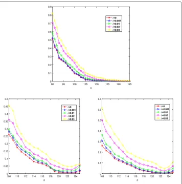
0.03, respectively, in this example. The regularizing parameters are selected asγ = 10–2_. The initial guess isφ0(x1,x2) = 0 andf0(x1,x2) = 0. We obtain the inverse results ofφ(x1,x2) andf(x1,x2), which are shown in Figs.4and5. In Fig.6, we give the numerical performance for noisy input data by giving the behavior ofJ(φδ

(14)

Figure 5Reconstructions of Example2: (ﬁrst line) exact and approximate solutions off(x1,x2) withδ= 0; (second line) approximate solutions forδ= 0.001, 0.01; (third line) approximate solutions forδ= 0.02, 0.03, respectively

err(fδ

n,f∗) with respect to the iteration numbernand noise levelδ(second line, (left) and (right)).

Remark4.1 The penalty termJ2can also be replaced byγ 2 2

T1 0

Ω|∇u|

2_dx_{, which means} that the heat ﬂux is bounded in physics. In comparison with J2used in this paper, the regularization eﬀect is more obvious for the inversion ofφ, and the number of iteration is decreasing. We have already tested it in 1-dimension.

5 Conclusion

(15)

measure-Figure 6Numerical performancesJ(φδ

n,fnδ) (ﬁrst line), err(φnδ,φ∗) (second line, (left)), err(fnδ,f∗) (second line,

(right)) with respect to the number of iterations forδ= 0, 0.001, 0.01, 0.02, and 0.03 of Example2

ment data at two diﬀerent times. The uniqueness and conditional stability results have been established. In Example1, we calculatedJ(φδ

n,fnδ),err(φδn,φ∗) anderr(fnδ,f∗) withδ= 0 by means of alternate and primary iteration schemes. In addition, the alternate iteration scheme takes 3 min, while the primary iteration scheme takes 5 min for 100 iterations in Matlab2016a. And as seen from Table1, by using the alternate iteration scheme, the value of functionalJ(φn,fn) is reduced faster than by the primary iteration scheme for the same number of iterations.

Acknowledgements

The authors would like to thank the anonymous referees for very helpful suggestions and comments which led to improvement of our original manuscript.

Funding

This work is supported by the Natural Science Foundation of Jiangsu Province of China (No. BK20181482), the Natural Science Foundation of the Jiangsu Higher Education Institutions of China (No. 18KJD110002) and the Scientiﬁc Research Foundation of Huaiyin Normal University (No. 31WBX00).

Competing interests

The authors declare that they have no competing interests.

Authors’ contributions

(16)

Publisher’s Note

Springer Nature remains neutral with regard to jurisdictional claims in published maps and institutional aﬃliations.

Received: 7 March 2019 Accepted: 16 September 2019 References

1. Evans, L.C.: Partial Diﬀerential Equations, 2nd edn. Am. Math. Soc., Providence (2010)

2. Colton, D.: The approximation of solutions to the backwards heat equation in a nonhomogeneous medium. J. Math. Anal. Appl.72, 418–429 (1979)

3. Liu, J.J.: Determination of temperature ﬁeld for backward heat transfer. Bull. Korean Math. Soc.16, 385–397 (2001) 4. Liu, J.J.: Numerical solution of forward and backward problem for 2-D heat conduction problem. J. Comput. Appl.

Math.145, 459–482 (2002)

5. Liu, J.J., Lou, D.J.: On stability and regularization for backward heat equation. Chin. Ann. Math., Ser. B24(1), 35–44 (2003)

6. Cheng, J., Liu, J.J.: A quasi Tikhonov regularization for a two-dimensional backward heat problem by a fundamental solution. Inverse Probl.24, 065012 (2008)

7. Liu, J.J., Wang, B.X.: Solving the backward heat conduction problem by homotopy analysis method. Appl. Numer. Math.128, 84–97 (2018)

8. Yan, L., Yang, F.L., Fu, C.L.: A meshless method for solving an inverse spacewise-dependent heat source problem. J. Comput. Phys.228(1), 123–136 (2009)

9. Johansson, B.T., Lesnic, D.: A variational method for identifying a spacewise-dependent heat source. IMA J. Appl. Math.72, 748–760 (2007)

10. Wang, Z.W., Wang, H.B., Qiu, S.F.: A new method for numerical diﬀerentiation based on direct and inverse problems of partial diﬀerential equations. Appl. Math. Lett.43, 61–67 (2015)

11. Xiong, X.T., Yan, Y.M.: A direct numerical method for solving inverse heat source problems. J. Phys. Conf. Ser.290, 012017 (2001)

12. Johansson, B.T., Lesnic, D.: A procedure for determining a spacewise dependent heat source and the initial temperature. Appl. Anal.87, 265–276 (2008)

13. Ye, Q.X., Li, Z.Y.: An Introduction to Reaction–Diﬀusion Equation. Science Press, Beijing (1994)

14. Isakov, V.: Inverse Problems for Partial Diﬀerential Equations, 2nd edn. Applied Mathematical Sciences, vol. 127. Springer, New York (2006)

15. Wang, Z.W., Qiu, S.F., Ruan, Z.S., Zhang, W.: A regularized optimization method for identifying the space-dependent source and the initial value simultaneously in a parabolic equation. Comput. Math. Appl.67, 1345–1357 (2014) 16. Shi, Z.: On the convergence of memory gradient method with Wolfe line search. Nonlinear Anal. Hybrid Syst.29, 9–18