Random non autonomous second order linear differential equations: mean square analytic solutions and their statistical properties

R E S E A R C H

Open Access

Random non-autonomous second order

linear differential equations: mean square

analytic solutions and their statistical

properties

J. Calatayud

_{, J.-C. Cortés}

_{, M. Jornet}

_{and L. Villafuerte}

*_{Correspondence:}

[email protected] 1_{Instituto Universitario de}

Matemática Multidisciplinar, Universitat Politècnica de València, Valencia, Spain

Full list of author information is available at the end of the article

Abstract

In this paper we study random non-autonomous second order linear differential equations by taking advantage of the powerful theory of random difference equations. The coefficients are assumed to be stochastic processes, and the initial conditions are random variables both defined in a common underlying complete probability space. Under appropriate assumptions established on the data stochastic processes and on the random initial conditions, and using key results on difference equations, we prove the existence of an analytic stochastic process solution in the random mean square sense. Truncating the random series that defines the solution process, we are able to approximate the main statistical properties of the solution, such as the expectation and the variance. We also obtain errora prioribounds to construct reliable approximations of both statistical moments. We include a set of numerical examples to illustrate the main theoretical results established throughout the paper. We finish with an example where our findings are combined with Monte Carlo simulations to model uncertainty using real data.

MSC: 39A50; 37H10; 34F05; 60H10; 60H35; 93E03; 65C05

Keywords: Random second order linear difference and differential equation; Analytic second order stochastic process;Lp_{() random calculus; Uncertainty} quantification; Mathematical modelling and stochastic computation

1 Introduction

In this paper, we take advantage of the powerful theory of random difference equations to conduct a full probabilistic study to the random second order linear differential equation

⎧ ⎪ ⎪ ⎨ ⎪ ⎪ ⎩ ¨

X(t) +A(t)X˙(t) +B(t)X(t) = 0, t∈R, X(t0) =Y0,

˙

X(t0) =Y1.

(1)

The data coefficientsA(t) andB(t) are stochastic processes and the initial conditionsY0

andY1are random variables on an underlying complete probability space (,F,P). In the

triple of the probability space,is the sample space, which consists of outcomes that will

be generically denoted byω;F is aσ-algebra of events; andPis a probability measure. Naturally, the solution of (1),X(t), is a stochastic process as well. Actually, we should write A(t,ω),B(t,ω),Y0(ω) andY1(ω), but to simplify the notation, and in concordance with the

literature, we will hide the generic outcomeωand just writeA(t),B(t),Y0andY1instead.

The aim of this paper is, in the first step, to specify the meaning of random differential equation (1) via the Lp_{() random calculus or, more concretely, using the so-called mean}

square calculus that corresponds top= 2; secondly, to find a proper stochastic process solution to (1); and thirdly, to compute its main statistical information (expectation and variance) under mild conditions.

Particular cases of the random initial value problem (1) have been studied in previous contributions using Lp_{() random calculus. For instance, important deterministic}

mod-els appearing in the area of mathematical physics like Airy, Hermite, Legendre, Laguerre and Bessel differential equations have been randomized and rigorously studied in [3,4,7,

8,10], respectively. In these contributions, approximate solution stochastic processes to-gether with their main statistical moments (mean and variance) are constructed by taking advantage of the random mean square calculus. Since in the case of Hermite, Legendre and Laguerre deterministic differential equations it is well known that they admit polynomial solutions, in those contributions the concept of random polynomial solution is introduced in the stochastic framework as well. In [15], the authors propose a homotopy technique to solve some particular random differential equations belonging to the class given in (1). A very important case of problem (1) is when its coefficients are random variables rather than stochastic processes, i.e.,A(t) =AandB(t) =B, corresponding to the autonomous case. In [6] the authors construct approximations of the first and second probability den-sity function of the solution stochastic process using a complementary approach to mean square calculus. In [13,14,18–20,33] one addresses significant advances for other random differential equations, dealing with the computation of the probability density function of the corresponding solution. Additional studies dealing with random differential equations via random mean square calculus include [12,21–24,26–28,31,36], for instance.

The structure of this paper is described as follows. In Sect.2we revise the notation and the theory of Lp_{() calculus necessary to understand the paper. In Sect.3we solve the}

random initial value problem (1) in a suitable way, and we describe the manner of approx-imating the main statistical information of the solution process (mean and variance). In Sect.4we compare our findings with the existing literature, and we also perform some numerical examples including an illustrative application in a modeling setting using real data. Finally, in Sect.5conclusions are drawn.

2 Preliminaries

Let (,F,P) be a complete probability space. In this paper we work with random variables X:→Rthat belong to the so-called Lebesgue spaces Lp_{(). Recall that we say that} X∈Lp_{(), 1≤p<∞, if the norm}

XLp₍₎:=

|X|pdP

1 p

is finite. We say thatX∈L∞() if the norm

XL∞():=inf sup X(ω):ω∈\N

is finite (this norm is usually termedessential supremum). These spaces are Banach, and the particular case of L2_{() is a Hilbert space. Sometimes, when we refer to convergence}

in L2(), we will say that the convergence holds in the mean square (m.s.) sense.

In general, the statistical information of the random variableXis given by a set of oper-ators that give information about the distribution ofX. In this paper we will deal with the expectation,E[X] =XdP, and with the variance,V[X] =E[(X–E[X])2]. Mean square convergence is important because it preserves the limit of the expectation and variance: if {Xn}∞n=1 is a sequence of random variables that converges in L2() toX (that is, m.s.

convergent), then

lim

n→∞E[Xn] =E[X], nlim→∞V[Xn] =V[X] (2)

(see Theorem 4.3.1 in [37]).

A very important inequality concerning the norm of a product of random variables is Hölder’s inequality: for any two random variables X and Y, we have XYLr₍₎ ≤ XLp()YLq(), where 1≤r,p,q≤ ∞and 1/r= 1/p+ 1/q. Whenr= 1 andp=q= 2,

the inequality is known as Cauchy–Schwarz inequality. Another stochastic result that will be used throughout this paper is Jensen’s inequality: if f is a convex function on

Rand assuming that the expectationsE[X] and E[f(X)] both exist and are finite, then f(E[X])≤E[f(X)]. In particular, iff(z) =|z|one gets|E[X]| ≤E[|X|].

In this paper we will also deal with stochastic processesX={X(t,ω) :t∈I,ω∈}, where I⊆R. To simplify notation, we will just writeXorX(t) and we will make the dependence onω∈implicit. Fixedω∈, the stochastic processX(t) can be seen as a real mapping fromI⊆RtoR, so any concept of real calculus, such as continuity, differentiability, etc., can be defined for the stochastic process.

However, sometimes it is more suitable to work with Lp_{() random calculus. In the case}

ofp= 2, it is termed mean square calculus. To read a full exposition on this topic, see [37, Ch. 4], [29, Ch. XI], or [30, Ch. 5]. In [38] the authors combine L2_{() and L}4_(),

corre-sponding to mean square and mean fourth random calculus, to solve random differential equations.

We say that the stochastic processXis in Lp_{() if the random variableX(t) belongs to}

Lp_{() for allt∈I. For such processes, we say thatXis differentiable in the L}p_{() sense at} t0∈Iif there exists a random variableX˙(t0) in Lp() such that

lim h→0

X(t0+h) –X(t0)

h –X˙(t0)

Lp₍₎ = 0.

The random variableX˙(t0) is called the Lp() derivative ofX(t) att0. We say that the

stochastic processXis differentiable onIin the Lp_{() sense if it is differentiable at every} t0∈I.

The stochastic processXis analytic att0ifX(t) = _∞

n=0Xn(t–t0)nfor everytin a

neigh-bourhood oft0, whereX0,X1, . . . are random variables and the sum is in the topology of

Lp_().

Thus, when we deal with the random differential equation (1), we will understand the derivatives in an Lp_{() random sense. More concretely, as we will see, the correct setting}

An important difference with respect to the deterministic scenario when solving a ran-dom differential equation is the computation of the main statistical functions associated to the solution stochastic process, such as the mean and the variance functions.

3 Results

Our main goal is to find the solution stochastic process to the random initial value prob-lem (1). We will assume that the data stochastic processA(t) andB(t) are analytic att0, in

the following sense:

A(t) =

∞

n=0

An(t–t0)n, B(t) = ∞

n=0

Bn(t–t0)n,

fort∈(t0–r,t0+r), beingr> 0 fixed, and the sum is understood in the L2() setting. We

search for an analytic solution processX(t) of the form

X(t) =

∞

n=0

Xn(t–t0)n,

fort∈(t0–r,t0+r), where the sum is in L2(). This stochastic process will be a solution

to the random problem (1) in the sense of L2() (so, in particular twice differentiable in the mean square sense).

3.1 Auxiliary results concerning random power series

We need some auxiliary results to deal with random power series in the L2_{() setting.}

First of all, we need a result to differentiate a power series in the Lp() sense (in this paper we will just use the casesp= 1 andp= 2, but we do the proof for a generalp≥1 just for the sake of completeness). The particular casep= 2 is a consequence of Theorem 3.1 in [11].

Theorem 3.1(Differentiation of a random power series in the Lp_{() sense) Let A(t) =}

∞

n=0An(t–t0)nbe a random power series in theLp()setting(p≥1)for t∈(t0–r,t0+r),

r> 0.Then the random power series∞_n=1nAn(t–t0)n–1exists inLp()for t∈(t0–r,t0+r);

moreover,theLp_{()derivative of A(t)is equal to it:}

˙

A(t) =

∞

n=1

nAn(t–t0)n–1

for all t∈(t0–r,t0+r).

Proof Let us see first that the random power series∞_n=1nAn(t–t0)n–1exists in Lp() for

t∈(t0–r,t0+r). Given 0 <ρ<r, we prove that

∞

n=1

nAnLp₍₎ρn–1<∞. (3)

Fixs: 0 <ρ<s<r. Since the sum∞_n=0Ansnexists in Lp(),limn→∞AnLp₍₎sn= 0, so there existsK> 0 such thatAnLp₍₎sn≤Kfor everyn≥0. Then

nAnLp₍₎ρn–1≤nK1 s

ρ s

n–1

As∞_n=1n(ρ/s)n–1_{<∞, by the comparison test for series, we conclude that (3) holds.}

Let us see now that the Lp_{() derivative ofA(t) is equal to}∞

n=1nAn(t–t0)n–1. By the

definition of Lp_{() derivative, we have to check that}

As it shall be apparent later, we need a theorem to multiply random power series. In the deterministic setting, the so-called Merten’s theorem allows multiplying two power series. The deterministic version of Merten’s theorem is proved in Theorem 8.46 of [1]. We adapt the proof in [1] to a stochastic setting in Theorem3.2. Notice that, from Theo-rem3.2, when we multiply two random power series, we lose Lebesgue spaces of conver-gence. As we will see in the proof, this fact will be a consequence of the Cauchy–Schwarz inequality (for two real numbersuandv, we always have|uv|=|u||v|; however, for ran-dom variablesU andV, we do not haveUVL2₍₎=U_L2₍₎V_L2₍₎ in general, but UVL1₍₎≤ U_L2₍₎V_L2₍₎).

Theorem 3.2(Merten’s theorem for random series in the mean square sense) Let U=

∞

n=0Unand V=

∞

n=0Vnbe two random series that converge inL2().Suppose that one of the series converges absolutely,say∞_n=0VnL2₍₎<∞.Then

cause of the Cauchy–Schwarz inequality, one gets

N→∞ (since by hypothesis

∞

n=0Vn

converges toV in L2()).

Thus, it only remains to prove that the second addend,N_m=0Vm

∞

n=N–m+1Un, goes to

SincelimN→∞∞n=NUn= 0 in L2(), there existsL> 0 such that

Then, forN≥2N, by the triangular inequality and the Cauchy–Schwarz inequality,

3.2 Main result: constructing the solution stochastic process of the random non-autonomous second order linear differential equation

We present the main theorem of this paper. After stating and proving it, a deeper analysis of the hypotheses and consequences of the theorem will be performed.

Theorem 3.3 Let A(t) =∞_n=0An(t–t0)nand B(t) = ∞

n=0Bn(t–t0)nbe two random series

in theL2_{()setting,for t∈(t}

0–r,t0+r),being r> 0finite and fixed.Assume that the initial

conditions Y0and Y1belong toL2().Suppose that there is a constant Cr> 0,maybe depen-dent on r,such thatAnL∞()≤Cr/rnandBnL∞()≤Cr/rn,n≥0.Then the stochastic

Proof Suppose thatX(t) =∞_n=0Xn(t–t0)nis a solution to (1) in the L2() sense fort∈

By the random Merten’s Theorem3.2,

A(t)X˙(t) =

IsolatingXn+2we obtain the recursive expression (8):

Xn+2= uniquely determined with probability 1.

It remains to check that the random series∞_n=0Xn(t–t0)nis convergent in L2(). For

that purpose, we will make use of the L∞() bounds forAnandBnquoted in the

hypothe-ses.

From the hypothesisY0,Y1∈L2() and by induction onnin expression (8), we obtain

thatXn∈L2() for alln≥0. By the triangular inequality, the hypotheses and Hölder’s

DefineH0:=Y0L2₍₎,H₁:=Y_1L2₍₎and

expressed as a function ofHn+1andHn(second order recurrence equation):

Hn+2=

3.3 Comments on the hypotheses of the theorem

The hypotheses concerning the L∞() growth of the coefficients An and Bn, n≥0,

may seem quite restrictive. However, these hypotheses have been necessary to relate the L2() norm of the coefficientsX0,X1,X2, . . . in (10), then define the random variables

H0,H1,H2, . . . and finally boundXnL2₍₎≤H_nby induction onn≥0. Without the hy-pothesesAnL∞()≤Cr/rnandBnL∞()≤Cr/rnof Theorem3.3, this would not have

been possible.

random variableZ, we have thatE[|Z|n_]≤HRn_{for certainH> 0 andR> 0 if and only if}

ZL∞()≤R.

This key fact is a direct consequence of the following result: ifZis a random variable, thenlim_n→∞ZLn₍₎=Z_L∞₍₎. For the sake of completeness, we show the proof. If obvious, we can assumeZ≡0). Then

lim sup n→∞ ZL

n₍₎≤ Z_L∞₍₎.

This shows the result whenZL∞()<∞. IfZL∞()=∞, then one has to defineL=

{|Z| ≥L}forL> 0 large. Proceeding similarly and by the arbitrariness ofL, one arrives at lim infn→∞ZLn₍₎=∞=Z_L∞₍₎.

Growth hypotheses of the formE[|Z|n_]≤HRn_{, for certainH> 0 andR> 0, are}

com-mon in the literature to find stochastic analytic solutions to particular cases of (1). See, for example, Airy’s random differential equation in [7] and Hermite’s random differential equation in [3]. We have proved in this subsection that controlling the growth of the mo-ments is equivalent to controlling the L∞() norm. Hence, Theorem3.3will allow us to generalize the results obtained in previous articles, for instance [3,7]. See Example4.1and Example4.2for the generalization.

3.4 Relationship between the random pointwise and classical differential equations approaches

The hypotheses of Theorem3.3, besides providing a stochastic solution to our problem (1), also give a pointwise classical solution to (1) under the additional assumptionY0,Y1∈

L∞(). Indeed, by hypothesis we havern_A

nL∞()≤CrandrnBnL∞()≤Cr. For fixed

δ> 0 small enough, one gets

From these two inequalities,

tion for eachω∈fixed (it is a solution from a deterministic point of view). This manner of studying random differential equations is referred to as the sample approach [37, Ap-pendix I], [9].

3.5 Statistical information of the solution stochastic process: mean and variance The expectation and variance of the stochastic processX(t) =∞_n=0Xn(t–t0)ngiven by

As an example of the manner one can proceed, we show by hand some random coeffi-cientsXn:

the expectation of the addends by hand:

E[X3] =

–1 6

E[A1]E[Y1] +E[B1]E[Y0] –E

A2₀E[Y1]

–E[A0]E[B0]E[Y0] +E[B0]E[Y1]

,

E[X4] =

–1 12

E[A2]E[Y1] +E[B2]E[Y0] –E[A1]E[A0]E[Y1] –E[A1]E[B0]E[Y0]

+E[B1]E[Y1] –

1

2E[A0]E[A1]E[Y1] – 1

2E[A0]E[B1]E[Y0] +1

2E

A3₀E[Y1] +

1 2E

A2₀E[B0]E[Y0] –

1

2E[A0]E[B0]E[Y1] –1

2E[B0]E[A0]E[Y1] – 1 2E

B2₀E[Y0]

.

For large values ofn, we need a computer to manage the big expressions forXn, and as a

consequenceE[XN(t)] andV[XN(t)] for large values ofN. We show how to implement the

necessary formulas to compute the expectation and variance of the truncated series in the software Mathematica®. The recurrence relation (7)–(8) is defined as follows:

X[n_?NonPositive] := Y0; X[1] = Y1;

X[n_] := -1/(n*(n - 1))*Sum[(m + 1)*A[n - 2 - m]*X[m + 1] + B[n - 2 - m]*X[m], {m, 0, n - 2}].

Truncation (14) is implemented by writing

seriesX[t_, t0_, N_] := X[0] + Sum[X[n]*(t - t0)^n, {n, 1, N}].

Using theExpectationfunction, in which one can set the distributions ofA[n],B[n], Y0andY1, both the expectation and variance of (14) can be calculated by the computer.

There are other approaches to approximating the expectation of the solution to the ran-dom initial value problem (1). One of these approaches is the so-called dishonest method [2], [17, p. 149], which assumes thatA(t) andX˙(t) are independent and thatB(t) andX(t) are independent. DenotingμX(t) =E[X(t)], the idea is that, sinceE[X¨(t)] = d

2

dt2(μX(t)) and

E[X˙(t)] = d

dt(μX(t)), because of the commutation between the mean square limit and the

expectation operator (see [37, Ch. 4]), by the assumed independence we arrive at a deter-ministic initial value problem to computeμX(t):

⎧ ⎪ ⎪ ⎨ ⎪ ⎪ ⎩

d2

dt2(μX(t)) +E[A(t)]_dd_t(μX(t)) +E[B(t)]μX(t) = 0, t∈R,

μX(t0) =E[Y0], d

dt(μX(t0)) =E[Y1].

(15)

In [2] and [17, p. 149] this method is used to handle the problem of computing the expec-tation of the solution stochastic process of certain random differential equations. In [3,

Another popular approach consists in using Monte Carlo simulations. Sample from the

Monte Carlo simulations, in contrast to the dishonest method, give always correct ap-proximations, and asMgrows, these approximations are more accurate, although Monte Carlo method possesses a slow convergence rate, namely,O(1/√M) [39, p. 53]. Thereby, the statistical information computed by means of Monte Carlo simulations must approx-imate our truncation method.

3.6 Obtaining error estimates for the approximation of the solution stochastic process, its mean and its variance

Given an error, we want to obtainNso thatXN(t) –X(t)L2₍₎<for allN≥N. Notice

that, in such a case, by Jensen’s and the Cauchy–Schwarz inequalities, we would have

_E

XN(t)

–EX(t)=EXN(t)–X(t)≤EXN(t)–X(t)≤XN(t)–X(t)_L2₍₎<, therefore we will be able to estimate the error when approximating the meanE[X(t)] via

E[XN(t)].

proof of Theorem3.3thatMn=Mfor sufficiently largen. In fact, fornsatisfying

ns because from these values we can see when (18) holds and computeHnvia the recursion

If we wantXN(t) –X(t)L2₍₎to be smaller than a prefixed error> 0, we impose

(here,xdenotes the least integer that is greater than or equal tox, commonly known as the ceiling ofx).

In Example4.1and Example4.4, we will apply these computations to find anN for

which the approximation ofE[X(t)] viaE[XN(t)] at the pointst= 1 andt= 0.25,

respec-tively, gives an error smaller than.

We develop a similar method to estimate the errors in the approximations for the vari-ance. That is to say, given an error> 0, we want to findNsuch that|V[XN(t)] –V[X(t)]|<

for allN≥N. We start bounding the difference|V[XN(t)] –V[X(t)]|using triangular,

Jensen’s and the Cauchy–Schwarz inequalities:

_V

≤δδ+ 2X(t)_L2₍₎

+δδ+ 2EX(t). To boundX(t)_L2₍₎, write

X(t)_L2₍₎=

∞

n=0

Xn(t–t0)n

L2₍₎ ≤

∞

n=0

XnL2₍₎ρn

≤

∞

n=0

Hnρn≤M

∞

n=0

ρ s

n

=M 1 1 –ρ_s =:γ,

whereρ=|t–t0|andsis any number satisfyingρ<s<r. Before, we saw how to compute

M, so we have obtained a computable bound forX(t)L2₍₎. On the other hand, to bound |E[X(t)]|we have two options. One option consists in using Jensen’s and the Cauchy– Schwarz inequalities to derive|E[X(t)]| ≤ X(t)L2₍₎≤γ, and we are done. The second option, which provides a tighter bound for|E[X(t)]|, consists in using the approximations performed forE[X(t)] viaE[XN(t)], and from them deducing an upper bound forE[X(t)].

For any of these two options, we denote the upper bound obtained for|E[X(t)]|byβ> 0. Thus, forN≥Nδ,

_V

XN(t)

–VX(t)≤δ(2γ+δ) +δ(2β+δ). Now chooseδso that

δ(2γ +δ) +δ(2β+δ)≤.

From here, we take

δ=–(γ +β) +

(γ+β)2_{+ 2}

2 > 0. (20)

To sum up, given a prefixed error> 0, the steps to be done in order to guarantee the approximationsV[XN(t)] of the exact varianceV[X(t)] to satisfy|V[XN(t)] –V[X(t)]| ≤

are the following ones:

1. Computeγ =M/(1 –ρ/s);

2. Computeβ> 0, upper bound of|E[X(t)]|; 3. Obtainδ> 0from (20);

4. TakeNδas in the approximation of the mean (expression (19), but withδinstead

of).

To put forward these ideas, in Example4.1and Example4.4we will apply these com-putations to find anNfor which, givena priorierror> 0, the approximation ofV[X(t)]

by means ofV[XN(t)] at the pointst= 1 andt= 0.25, respectively, gives an error smaller

than.

4 Examples

dishonest method and Monte Carlo simulations. We will compare the three approaches in order to realize the potentiality of using the truncation method. Our truncation method and Monte Carlo simulation must give similar approximations of the statistical moments (and equal and exact results in the limit).

In addition, we will take some particular problems (1) that have been already studied in the literature such as Airy’s and Hermite’s random differential equations [3,7]. As we will see, our findings will generalize the results obtained in those papers (recall Sect.3.3).

Example4.1 (Airy’s random differential equation) Airy’s random differential equation is the following:

⎧ ⎪ ⎪ ⎨ ⎪ ⎪ ⎩ ¨

X(t) +AtX(t) = 0, t∈R, X(0) =Y0,

˙

X(0) =Y1,

(21)

whereA,Y0andY1are random variables.

In [7], the hypothesis used in order to obtain a mean square analytic solution X(t) isE[|A|n_]≤HRn_,n≥n

0. Notice that this hypothesis is equivalent toAL∞()≤Rby

Sect.3.3.

In the caseE[|A|n_]≤HRn_,n≥n

0(that is,AL∞()≤R), we are under the hypotheses

of Theorem3.3. Indeed, in the notation of Theorem3.3,An= 0 for alln≥0,B1=Aand

Bn= 0 for everyn= 1. For a fixed and finiter> 0 andt0= 0, we haveB1L∞()≤Cr/r1,

beingCr=rAL∞(), for instance. Then the stochastic processX(t) = ∞

n=0Xntn, defined

as in Theorem3.3, is a mean square analytic solution to (21) in (–r,r). Asr> 0 is arbitrary, in factX(t) =∞_n=0Xntnis a mean square analytic solution to (21) inR.

Let us carry out a practical case. As in [7], considerA∼Beta(2, 3) andY0,Y1

indepen-dent random variables such thatY0∼Normal(1, 1) andY1∼Normal(2, 1). Tables1and2

collect the simulations obtained in [7]. In Table1we show, for distinct values oft,E[XN(t)]

forN= 15 andN= 16, the expectation of the solution stochastic process obtained via the dishonest method and also using Monte Carlo simulations with samples of size 50,000 and 100,000. In Table2we present, for distinct values oft,V[XN(t)] forN= 15 andN= 16 and

the corresponding approximations computed via Monte Carlo sampling with 50,000 and 100,000 simulations.

We observe that convergence has been achieved for smallN. Compare with Monte Carlo simulation, in which a lot of realizations are required in order to obtain good approxima-tions. Nevertheless, it must be remarked that smallNis needed for the truncation order, because Airy’s random differential equation is not specially complex. For more complex data processes, as in Example4.3, Example4.4and Example4.5, a larger order of trunca-tionNmay be needed. This may imply a computational expense greater than or similar to Monte Carlo simulation.

On the other hand, it is remarkable how well the dishonest method approximates the correct expectation, although the required independence betweenA(t),X˙(t) andB(t),X(t) does not hold. The key point is thatCov[A(t),X˙(t)] andCov[B(t),X(t)] are small, as Table3

shows, which justifies the accuracy of the dishonest method, especially for smallt. Notice that, in this example,Cov[A(t),X˙(t)] = 0, becauseA(t)≡0 is deterministic. The value of

Table 1 Approximation of the expectation of the solution stochastic process. Example4.1, assuming independent random data

t E[X15(t)] E[X16(t)] Dishonest MC 50,000 MC 100,000

0.00 1 1 1 0.99701 1.00138

0.25 1.49870 1.49870 1.49870 1.49519 1.49976

0.50 1.98752 1.98752 1.98752 1.98353 1.98829

0.75 2.45108 2.45108 2.45102 2.44667 2.45160

1.00 2.86856 2.86856 2.86818 2.86383 2.86893

1.25 3.21494 3.21494 3.21339 3.21008 3.21534

1.50 3.46310 3.46310 3.45812 3.45831 3.46376

1.75 3.58660 3.58660 3.57340 3.58215 3.58784

2.00 3.56336 3.56335 3.53286 3.55948 3.56552

Table 2 Approximation of the variance of the solution stochastic process. Example4.1, assuming

independent random data

t V[X15(t)] V[X16(t)] MC 50,000 MC 100,000

0.00 1 1 0.99610 0.99530

0.25 1.06035 1.06035 1.05902 1.05642

0.50 1.23142 1.23142 1.23408 1.22793

0.75 1.49261 1.49261 1.50041 1.48944

1.00 1.81392 1.81392 1.82744 1.81127

1.25 2.15870 2.15870 2.17768 2.15721

1.50 2.49379 2.49379 2.51690 2.49462

1.75 2.80560 2.80560 2.83029 2.81030

2.00 3.11530 3.11530 3.13783 3.12559

Table 3 Approximation ofCov[A(t),X(t)] and˙ Cov[B(t),X(t)] via accurate truncationsX˙₁₆(t) andX₁₆(t),

respectively. Example4.1, assuming independent random data

t Cov[A(t),X˙16(t)] Cov[B(t),X16(t)]

0.00 0 0

0.25 0 –0.0000325384

0.50 0 –0.000622983

0.75 0 –0.00365252

1.00 0 –0.0130099

1.25 0 –0.0349332

1.50 0 –0.0778424

1.75 0 –0.151444

2.00 0 –0.264968

since for this order of truncation one gets good approximations ofX(t); in other words, approximations can be consider as fairly exact.

We perform another example of Airy’s random differential equation (21), but this time the input random variablesA,Y0andY1will not be independent. Indeed, take a random

vector (A,Y0,Y1) that follows a multivariate Gaussian distribution, with mean vector and

covariance matrix

μ=

⎛ ⎜ ⎝

0.4 1 2

⎞ ⎟

⎠, =

⎛ ⎜ ⎝

0.04 0.0001 –0.05 0.0001 1 0.5 –0.005 0.5 1

⎞ ⎟ ⎠,

Table 4 Approximation of the expectation of the solution stochastic process. Example4.1, assuming dependent random data

t E[X15(t)] E[X16(t)] Dishonest MC 50,000 MC 100,000

0.00 1 1 1 1.00287 1.00114

0.25 1.50619 1.50619 1.49870 1.50202 1.50134

0.50 1.98755 1.98755 1.98750 1.99129 1.99168

0.75 2.45120 2.45120 2.45102 2.45529 2.45678

1.00 2.86893 2.86893 2.86818 2.87321 2.87583

1.25 3.23538 3.23538 3.21339 3.22008 3.22386

1.50 3.46485 3.46485 3.45812 3.46878 3.47374

1.75 3.58966 3.58966 3.57340 3.59290 3.59902

2.00 3.56817 3.56817 3.53286 3.57032 3.57755

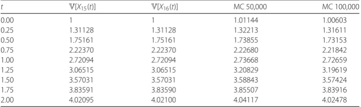
Table 5 Approximation of the variance of the solution stochastic process. Example4.1, assuming

dependent random data

t V[X15(t)] V[X16(t)] MC 50,000 MC 100,000

0.00 1 1 1.01144 1.00603

0.25 1.31128 1.31128 1.32213 1.31611

0.50 1.75161 1.75161 1.73855 1.73153

0.75 2.22370 2.22370 2.22680 2.21842

1.00 2.72094 2.72094 2.73668 2.72659

1.25 3.06515 3.06515 3.20829 3.19619

1.50 3.57031 3.57031 3.58843 3.57424

1.75 3.83591 3.83590 3.85507 3.83916

2.00 4.02095 4.02100 4.04117 4.02478

Table 6 Approximation ofCov[A(t),X(t)] and˙ Cov[B(t),X(t)] via accurate truncationsX˙16(t) andX16(t),

respectively. Example4.1, assuming dependent random data

t _Cov[A(t),X˙16(t)] Cov[B(t),X16(t)]

0.00 0 0

0.25 0 –0.00106042

0.50 0 –0.00177052

0.75 0 –0.00618508

1.00 0 –0.0173

1.25 0 –0.0509053

1.50 0 –0.0858552

1.75 0 –0.161068

2.00 0 –0.276206

contains 99.7%of the observations ofA. Thus, the multivariate Gaussian distribution will be truncated to [–0.2, 1]×R×R.

In Tables4and5, we present the numerical experiments. We use truncation (14) with N= 15 andN= 16, the dishonest method and Monte Carlo simulation.

Once again, convergence has been achieved quite quickly compared with Monte Carlo simulation. The results obtained are more accurate than via the dishonest method and Monte Carlo simulation. Nonetheless, the accuracy of the dishonest method is remarkable again, particularly in the time intervalt∈[0, 1], although not as good as in the previous case (see Table1). In Table6, we show approximations of the covariancesCov[A(t),X˙(t)] andCov[B(t),X(t)]. These covariances are small, especially for smallt, which explains the good approximation of the expectation via the dishonest method.

= 0.00001. Taket= 1 andr= 2. Let, for instance,s= 1.5. In both cases in this exam-ple (assuming independent and dependent random data), we haveCr=rAL∞(). Since

AL∞()= 1 (recall that in the two cases considered throughout this example, the

re-alizationsA(ω),ω∈, of the random variableAlie either in [0, 1] or in [–0.2, 1], thus being less than 1), we takeCr=r= 2. From these values, the leastn0such that (18) holds

for alln≥n0isn0= 7 (this value is obtained by plotting the left-hand side of (18) and

looking at the pointn0from which the graph is less than 1). Then, from (13),M=M8=

max_0≤m≤8Hmsm= 2024.49. Finally, using (19), one getsN= 10. ForN≥N= 10, it holds

|E[XN(t)] –E[X(t)]|< 0.00001.

Now, given= 0.00001, we obtain anN such that|V[XN(t)] –V[X(t)]|< att= 1 for

everyN≥N. We use the ideas and notation from Sect.3.6. We havet= 1,ρ= 1,r= 2 and

s= 1.5. We saw thatM= 2024.49. Thenγ =M/(1 –ρ/s) = 6073.47. Recall that we could chooseβ equal toγ or, for a tighter bound, use Tables1and4. We see that|E[X(t)]| ≤ 2.869 =:β. From these values, we obtainδ= 8.22638·10–10. Finally, chooseNδ so that

XN(1) –X(1)L2₍₎<δ. Use formula (19) (withδ instead of) to getNδ= 73. Thus, for

N≥73, the inequality|V[XN(t)] –V[X(t)]|< 0.00001 holds for sure.

Example 4.2 (Hermite’s random differential equation) Hermite’s random differential equation is defined as follows:

⎧ ⎪ ⎪ ⎨ ⎪ ⎪ ⎩ ¨

X(t) – 2tX˙(t) +AX(t) = 0, t∈R, X(0) =Y0,

˙

X(0) =Y1,

(22)

whereA,Y0andY1are random variables.

In [3], the moments ofAare controlled asE[|A|n_]≤HRn_,n≥n

0, to prove the existence

of a mean square analytic solution to random initial value problem (22). As we saw in Sect.3.3, this hypothesis reduces toAL∞()≤R.

IfE[|A|n]≤HRn,n≥n0(that is,AL∞()≤R), we are under the assumptions of

The-orem3.3. Indeed, in the notation of Theorem3.3,A1= –2,An= 0 for alln= 1,B0=Aand

Bn= 0 for everyn= 0. For a fixed and finiter> 0 andt0= 0, we haveA1L∞()≤Cr/r1and

B0L∞()≤Cr/r0=Cr, beingCr=max{2r,AL∞()}for example. ThenX(t) = ∞

n=0Xntn

defined as in Theorem3.3is an analytic solution to (22) in (–r,r). Again, asr> 0 is arbi-trary,X(t) =∞_n=0Xntnis a mean square analytic solution stochastic process to random

initial value problem (22) inR.

As in [3], letA∼Normal(μ= 5,σ2_{= 1) andY}

0,Y1independent random variables such

thatY0∼Normal(1, 1) andY1∼Normal(2, 1). In this case, since the normal distribution

is unbounded, it does not fulfill the hypotheses, therefore we need to truncate it: in [3] it has been truncated to the interval [μ– 3σ,μ+ 3σ] = [2, 8], which contains approxi-mately 99.7%of the observations of a Gaussian random variable. Tables7and8simulate the results obtained in [3]. In Table7we show, for distinct values oft,E[XN(t)] forN= 15

andN = 16, the corresponding approximation obtained via the dishonest method and Monte Carlo simulations with samples of size 50,000 and 100,000. In Table8we present, for distinct values oft,V[XN(t)] forN= 15 andN= 16 and Monte Carlo simulations with

Table 7 Approximation of the expectation of the solution stochastic process. Example4.2

t E[X15(t)] E[X16(t)] Dishonest MC 50,000 MC 100,000

0.00 1 1 1 0.99750 0.99919

0.25 1.32907 1.32907 1.32889 1.32619 1.32703

0.50 1.26473 1.26473 1.26175 1.26351 1.26219

0.75 0.74510 0.74510 0.72906 0.74737 0.74316

1.00 –0.27157 –0.27157 –0.32467 –0.26484 –0.27144

1.25 –1.80636 –1.80635 –1.93991 –1.79597 –1.80237

1.50 –3.85882 –3.85868 –4.13681 –3.84872 –3.84906

1.75 –6.40911 –6.40754 –6.90081 –6.40873 –6.39186

2.00 –9.43553 –9.42222 –10.1448 –9.46498 –9.41066

Table 8 Approximation of the variance of the solution stochastic process. Example4.2

t V[X15(t)] V[X16(t)] MC 50,000 MC 100,000

0.00 1 1 0.98671 1.00327

0.25 0.77433 0.77433 0.76716 0.77821

0.50 0.37752 0.37752 0.37822 0.37992

0.75 0.54181 0.54181 0.53554 0.54357

1.00 2.10396 2.10396 2.06444 2.10993

1.25 5.48674 5.48670 5.40047 5.50378

1.50 10.4476 10.4467 10.3456 10.4828

1.75 18.0186 18.0108 17.9539 18.0963

2.00 43.5731 43.6462 43.5773 44.1340

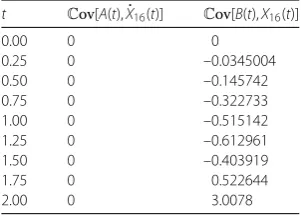
Table 9 Approximation ofCov[A(t),X(t)] and˙ Cov[B(t),X(t)] via accurate truncationsX˙16(t) andX16(t),

respectively. Example4.2

t Cov[A(t),X˙16(t)] Cov[B(t),X16(t)]

0.00 0 0

0.25 0 –0.0345004

0.50 0 –0.145742

0.75 0 –0.322733

1.00 0 –0.515142

1.25 0 –0.612961

1.50 0 –0.403919

1.75 0 0.522644

2.00 0 3.0078

Cov[A(t),X˙(t)] and Cov[B(t),X(t)] to understand better the accuracy of the dishonest method.

Example4.3 (Random linear differential equation with polynomial data processes) Let us consider more complex data processes in our random differential equation (1). The data stochastic processes will be random polynomials. For example,

⎧ ⎪ ⎪ ⎨ ⎪ ⎪ ⎩ ¨

X(t) + (A0+A1t)X˙(t) + (B0+B1t)X(t) = 0, t∈R,

X(0) =Y0,

˙

X(0) =Y1,

(23)

whereA0= 4,A1∼Uniform(0, 1),B0∼Gamma(2, 2),B1∼Bernoulli(0.35),Y0= –1 and

Y1∼Binomial(2, 0.29) are assumed to be independent. In order for the hypotheses of

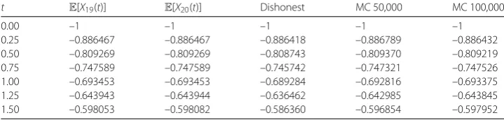
distri-Table 10 Approximation of the expectation of the solution stochastic process. Example4.3

t E[X19(t)] E[X20(t)] Dishonest MC 50,000 MC 100,000

0.00 –1 –1 –1 –1 –1

0.25 –0.886467 –0.886467 –0.886418 –0.886789 –0.886432

0.50 –0.809269 –0.809269 –0.808743 –0.809370 –0.809219

0.75 –0.747589 –0.747589 –0.745742 –0.747321 –0.747526

1.00 –0.693453 –0.693453 –0.689284 –0.692816 –0.693375

1.25 –0.643943 –0.643944 –0.636462 –0.642985 –0.643845

1.50 –0.598053 –0.598082 –0.586360 –0.596854 –0.597952

Table 11 Approximation of the variance of the solution stochastic process. Example4.3

t V[X15(t)] V[X16(t)] MC 50,000 MC 100,000

0.00 0 0 0 0

0.25 0.0102077 0.0102074 0.0101172 0.0102664

0.50 0.0190996 0.0190999 0.0189214 0.0192053

0.75 0.0237400 0.0237403 0.0235191 0.0238499

1.00 0.0268721 0.0268711 0.0266311 0.0269620

1.25 0.0297852 0.0297465 0.0295049 0.0298201

1.50 0.0333309 0.0325867 0.0325021 0.0328009

bution with shape and rate 2, it can straightforwardly be checked that the interval [0, 4] contains approximately 99.7%of the observations.

By Theorem3.3, the mean square solution of (23) can be written as a random power seriesX(t) =∞_n=0Xntnthat is mean square convergent for allt∈R.

In Tables10and11, the numerical experiments for the expectation and variance are presented.

Example4.4 (Random linear differential equation with infinite series data processes) In this example, the data stochastic processes in the random differential equation (1) are non-polynomial analytic stochastic process:

⎧ ⎪ ⎪ ⎨ ⎪ ⎪ ⎩ ¨

X(t) +A(t)X˙(t) +B(t)X(t) = 0, t∈R, X(0) =Y0,

˙

X(0) =Y1,

(24)

where An∼Beta(11, 15) forn≥0,Bn= 1/n2, forn≥1, andY0∼Poisson(2) and Y1∼

Uniform(0, 1) are assumed to be independent. We have E[An] = 11/26 and V[An] =

55/6084, thereforeAnL2₍₎=

V[An] +E[An]2= 0.12908,n≥0. Then

∞

n=0

AnL2₍₎tn= 0.12908

∞

n=0

tn,

which is convergent fort∈(–1, 1). On the other hand,

∞

n=0

BnL2₍₎tn=

∞

n=1

1 n2t

n_,

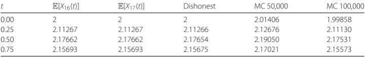
Table 12 Approximation of the expectation of the solution stochastic process. Example4.4, assuming independent initial conditions

t E[X16(t)] E[X17(t)] Dishonest MC 50,000 MC 100,000

0.00 2 2 2 2.01406 1.99858

0.25 2.11267 2.11267 2.11266 2.12676 2.11130

0.50 2.17662 2.17662 2.17654 2.19050 2.17531

0.75 2.15693 2.15693 2.15675 2.17021 2.15573

Table 13 Approximation of the variance of the solution stochastic process. Example4.4, assuming

independent initial conditions

t V[X17(t)] V[X18(t)] MC 50,000 MC 100,000

0.00 2 2 2.00274 2.00822

0.25 1.99421 1.99421 1.99725 2.00356

0.50 1.93408 1.93408 1.93725 1.94407

0.75 1.76917 1.76919 1.77222 1.77899

Since|An(ω)| ≤1 for allω∈,|Bn| ≤1 andr= 1, we can takeCr= 1 in Theorem3.3and

the hypotheses hold. By Theorem3.3, the mean square solution of (24),X(t), is defined and is mean square analytic on (–1, 1).

In Tables 12and13 we present the numerical experiments. To apply the dishonest method, we need the following two computations:

EA(t)=11 26

∞

n=0

tn= 11

26(1 –t), t∈(–1, 1)

and

EB(t)=

∞

n=1

tn

n2, t∈(–1, 1).

To apply Monte Carlo simulation, we need realizations of the stochastic processA(t), that is, realizations of the random variablesA0,A1, . . . . As we cannot obtain infinite

realiza-tions of a beta distribution in the computer, we will approximateA(t,ω)≈100_n=0An(t,ω)tn.

So, from realizations ofA0, . . . ,A100, we will obtain an approximation of a realization of

A(t).

By contrast, our approximations using truncationXN(t),t∈(–1, 1), do not require

real-izations of the infinite data stochastic processA(t).

As it is observed in Tables12and13, the convergence has been practically achieved for N= 17.

As an application of the error estimates analyzed in Sect.3.6, we estimate for which indexNthe error obtained in the approximation ofE[X(t)] viaE[XN(t)] is smaller than

= 0.00001. Taket= 0.25 and, for instance,s= 0.5. We haver= 1 andCr= 1, and from

these values we obtain the leastn0such that (18) holds for alln≥n0by trial and error.

We obtainn0= 0. From (13),M=M1=max{H0,H1s}=max{Y0L2₍₎,Y_1L2₍₎·0.5}=

max{√6, 1/(2√3)}=√6, whenceN= 18 by using (19).

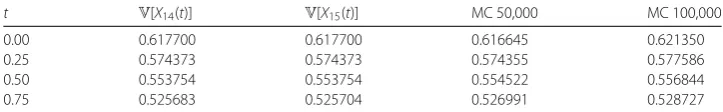
Table 14 Approximation of the expectation of the solution stochastic process. Example4.4, assuming dependent initial conditions

t E[X15(t)] E[X16(t)] Dishonest MC 50,000 MC 100,000

0.00 0.87 0.87 0.87 0.866780 0.869210

0.25 0.973828 0.973828 0.973819 0.970205 0.973499

0.50 1.04817 1.04817 1.0481 1.04427 1.04823

0.75 1.07358 1.07358 1.0734 1.06961 1.07394

Table 15 Approximation of the variance of the solution stochastic process. Example4.4, assuming

dependent initial conditions

t V[X14(t)] V[X15(t)] MC 50,000 MC 100,000

0.00 0.617700 0.617700 0.616645 0.621350

0.25 0.574373 0.574373 0.574355 0.577586

0.50 0.553754 0.553754 0.554522 0.556844

0.75 0.525683 0.525704 0.526991 0.528727

ands= 0.5. We computedM=√6, whence γ =M/(1 –ρ/s) = 4.89898. Recall that we could chooseβ equal toγ or, for a tighter bound, use Table12. In Table12, we see that |E[X(0.25)]| ≤2.113 =:β. From these values,δ= 7.13065·10–7. To end up, pickNδ such

thatXN(0.25) –X(0.25)L2₍₎<δ. Using expression (19) (withδinstead of), we getNδ=

22. Thereby,|V[XN(0.25)] –V[X(0.25)]|< 0.00001 forN≥22.

We perform another example for the random initial value problem (24), again with An∼Beta(11, 15) forn≥0,Bn= 1/n2forn≥1, but now the random vector (Y0,Y1)

fol-lows a multinomial distribution with three repetitions and probabilities 0.29 and 0.15. The random variables/vectorsA0,A1, . . . and (Y0,Y1) are independent, but, obviously,Y0and

Y1are not independent. Again, the solution stochastic processX(t) is defined on (–1, 1).

In Tables14and15, we show the numerical experiments. Convergence has been prac-tically achieved.

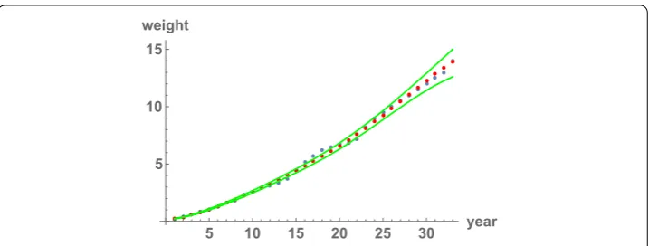
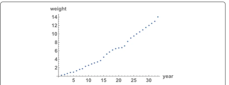
Example4.5 (An application of the truncation method and Monte Carlo simulation to modeling) In order to see a real application of our theoretical development, let us fit data that describe the fish weight growth over the time via a random second order linear differ-ential equation. In Fig.1, we show the fish weight in lbs (vertical axis) per year (horizontal axis). The fish weight datum at theith year will be denoted bywifor 1≤i≤33.

These data were previously used in [5], where a randomized Bernoulli differential equa-tion was used, taking as reference the Bertalanffy model [34, p. 331].

LetWbe the stochastic process that models the fish weight. The random variableW(t) models the fish weight at yeart, 1≤t≤33. SinceW(t) is a positive random variable, we will work withX(t) =log(W(t)) instead. The observed data becomelog(w1), . . . ,log(w33).

We use the random initial value problem

⎧ ⎪ ⎪ ⎨ ⎪ ⎪ ⎩ ¨

X(t) +A0X˙(t) + (B0+B1t)X(t) = 0, t∈R,

X(0) =Y0,

˙

X(0) =Y1

(25)

to model the logarithm of the fish weight growth. The stochastic processesA(t) =A0and

B(t) =B0+B1thave been chosen by numerical fit trials and computational viability. Notice

Figure 1Data on fish weights. In the horizontal axis, we represent the years, from 1 to 33. In the vertical axis, we represent the weights in lbs

Using the data drawn in Fig.1, we would like to find the best random variablesA0,B0,

B1,Y0andY1so thatW(t) fits appropriately the uncertainty associated to the fish weight

growth. Since we do not have an explicit solution processX, we will use truncation (14), XN(t), to approximate it in the L2() sense. Using the truncation with a highN, we will be

able to give a suitable distribution for (A0,B0,B1,Y0,Y1).

There are two statistical approaches to dealing with this problem: the frequentist and the Bayesian techniques. Reference [25] provides an introduction to Bayesian statistics. We do not carry out a Bayesian approach, becauseXN(t) has a very large expression, which makes

the use of Bayesian estimation impracticable in the computer. Thereby, we use the ideas of the so-called inverse frequentist technique for parameter estimation exhibited in [5] and [35, Chap. 7]. In order not to depart from our reasoning, we will explain our concrete frequentist approach in Remark4.6at the end of this example.

Without entering into the theoretical details that will be explained in Remark4.6, we specify the steps to solve our modeling problem. Computational viability makes us choose N= 24 as the order of truncation. We give the random vector (A0,B0,B1,Y0,Y1) a sixth

dimensional multinormal random distribution (in the end, it will be truncated so that the hypotheses of Theorem3.3are fulfilled). The mean vectorμis determined as the solution of the deterministic minimization problem

min a0,b0,b1,y0,y1∈R

33

i=1

log(wi) –X24(ti|a0,b0,b1,y0,y1) 2

,

whereX24(t|a0,b0,b1,y0,y1) corresponds to the value ofX24(t) substitutingA0,B0,B1,Y0

andY1by the real numbersa0,b0,b1,y0andy1. This minimization problem can be solved

with the built-in functionFindFitwith the optionMethod -> NMinimizein Mathe-matica®. We obtain

μ=

⎛ ⎜ ⎜ ⎜ ⎜ ⎜ ⎜ ⎝

0.169695 –0.0123653 0.000347771

–2.09309 0.672599

⎞ ⎟ ⎟ ⎟ ⎟ ⎟ ⎟ ⎠

Figure 2Fit of the fish weight data. The blue points represent the real weights, the red points represent the estimated weights (the mean) and the green lines cover a 95% confidence interval constructed with the Gaussian rule [mean_±2_·standard deviation]

The covariance matrixis estimated withσ2(JTJ)–1_{, where}

σ2=

33

i=1(log(wi) –X24(ti|μ))2

33 – 5 = 0.00369358,

andJis the Jacobian matrix ofX24(t) with respect to (A0,B0,B1,Y0,Y1) evaluated atμ. We

obtain

=

⎛ ⎜ ⎜ ⎝

0.000109461 –0.000010458 1.44986·10–7 _{–0.000645456 0.000435313}

–0.000010458 2.47732·10–6 _{–7.94312·10}–8 _{0.0000461867 –0.0000398354}

1.44986·10–7 _{–7.94312·10}–8 _3.23082·10–9 _{–3.16049·10}–7 _5.53045·10–7

–0.000645456 0.0000461867 –3.16049·10–7 _{0.00624016 –0.00312264}

0.000435313 –0.0000398354 5.53045·10–7 _{–0.00312264 0.00186506} ⎞ ⎟ ⎟ ⎠.

Once we know the estimated distribution of the random vector (A0,B0,B1,Y0,Y1), we

know the distribution ofX24(t), at least theoretically. The computational complexity of

X24(t) is very big, so computing its exact expectation or even good approximations of it is

nearly impossible. Due to the complexity of both the truncation expression and the dis-tribution of (A0,B0,B1,Y0,Y1), it is better to perform Monte Carlo simulation directly on

(25) via simulations of (A0,B0,B1,Y0,Y1), which follows a (truncated) multivariate

Gaus-sian distribution (μ,).

By means of Monte Carlo simulation with 100,000 iterates, we obtain samples ofX(i), i= 1, . . . , 33. Applying exponential, we have samples ofW(i),i= 1, . . . , 33. Hence, approx-imations of both E[W(i)] andV[W(i)] can be calculated. A confidence interval can be computed in two ways: either considering [E[W(t)]±2√V[W(t)]] (this is based on how confidence intervals are constructed in a Gaussian setting) or obtaining an accurate ap-proximation using the quartiles of the sample produced by Monte Carlo. In Figs.2and3, the results are shown. As it is observed in both plots, the mean approximates well the real data. However, the confidence interval grows as we move away from 0. Intuitively, this may hold because a truncated random power series centered att0works better neart0.

This phenomenon may be resolved by making the order of truncationNlarger and larger (if the computer permits it).

Figure 3Fit of the fish weight data. The blue points represent the real weights, the red points represent the estimated weights (the mean) and the green lines cover a 95% confidence interval constructed by taking the quartiles in the Monte Carlo sampling

X=f(V), whereVis a random vector withpcomponents (in our case (A0,B0,B1,Y0,Y1))

that follows a multinormal distribution with parameters (μ,), andf :Rp_→Rn_{is a}

func-tion, maybe non-linear (in our case,n= 33 andfi(a0,b0,b1,y0,y1) =X24(i|a0,b0,b1,y0,y1),

i= 1, . . . , 33, whereX24(t|a0,b0,b1,y0,y1) is the truncation that approximates the solution

of the random differential equation). Letx=X(ω) be a vector realization ofX(in our ex-ample, the real datax= (log(w1), . . . ,log(w33))). Fromx, we want to estimate the bestμand

so that the modelX=f(V) can be considered correct. Letvˆ∈Rp_{be the minimizer of}

min v∈Rp

n

i=1

xi–fi(v)

2

.

Using Taylor’s expansion,

X≈f(vˆ) +Jf(vˆ)(V–vˆ),

whereJstands for the Jacobian. Then

Z:=X–f(vˆ) +Jf(vˆ)ˆv≈Jf(ˆv)

J V.

We derive thatZ≈Jμ+E, whereEfollows a multivariate normal distribution with param-eters (0,JJT_{) (hereT stands for the transpose matrix operator), i.e.,E∼MN(0,JJ}T_).

WriteJJT_=PT_{DP, wherePandDare an orthogonal and a diagonal matrix, respectively.}

Multiplying byP, we haveZ¯≈ ¯Jμ+E¯, whereZ¯=PZ,¯J=PJandE¯=PE∼MN(0,D). There-fore,Z¯ ≈ ¯Jμ+E¯ is a classical linear model (see [32, Chap. 7], [35, Chap. 7]) with normal and independent errors. In a linear model, one should assume homoscedasticity so that the estimation of the parameters makes sense. Thus, we imposeD=σ2In, whereσ2is the

variance of the errors in the linear model. As a consequence,Z¯ ≈ ¯Jμ+E¯ is a classical lin-ear model with homoscedasticity, and the estimations follow from general theory:μˆis the minimizer of

min

μ∈Rp¯z–¯Jμ

2

2=_μ∈min_RpPz–PJμ

2

2=_μ∈min_Rpz–Jμ

wherez=x–f(vˆ) +Jvˆis the vector realization ofZ,¯z=Pzis the vector realization ofZ¯ and · 2is the Euclidean norm. Now,

z–Jμ2₂=x–f(vˆ) +J(μ–vˆ)2₂≈x–f(μ)2₂,

so we can takeμˆ=ˆv, which justifies our choice for the mean in the example. On the other hand, by the general theory of linear models,

ˆ

σ2=¯z–¯Jμˆ

2 2

n–p =

Pz–PJμˆ2 2

n–p =

z–Jμˆ2 2

n–p ≈

x–f(μ)ˆ 2 2

n–p .

Finally, fromJJT_=PT_DP=σ2_PT_P=σ2_I

n, we derive=σ2(JTJ)–1, by multiplying by

(JTJ)–1_JT_{to the left and byJ(J}T_J)–1 _{to the right at both sides of the equality (we assume}

rank(J) =pso that (JTJ)–1exists). Thus, we choose the estimatorˆ =σˆ2(JTJ)–1.

5 Conclusions

In this paper we have determined analytic stochastic processes that are solutions to the random non-autonomous second order linear differential equation in the mean square sense taking advantage of the powerful theory of random difference equations. After re-viewing the Lp_{() random calculus and results concerning random power series}

(differ-entiation of a random power series in the Lp_{() sense and Merten’s theorem for random}

series in the mean square sense), we stated the main theorem of the paper, Theorem3.3. This theorem gives assumptions on the coefficient stochastic processes and on the random initial conditions of a random non-autonomous second order linear differential equation, so that there exists an analytic stochastic process that is a solution in the mean square sense. This mean square approach permitted approximating the main statistical informa-tion of the soluinforma-tion stochastic process, expectainforma-tion and variance. These approximainforma-tions for the expectation and variance were compared with other methods previously used in the literature: the dishonest method and Monte Carlo simulation.

The numerical examples presented illustrate the potentiality of our results. The exam-ples show that our findings allow for much more complex random non-autonomous sec-ond order linear differential equations than those from the existing literature. The ideas of this paper permit dealing with any random non-autonomous second order linear dif-ferential equation in a general form. The statistical information of the stochastic process solution can be computed up to any degree of accuracy. These achievements have been reached thanks to the powerful theory of difference equations.

Moreover, our truncation method provides a methodology to estimate the parameters of the multivariate normally distributed explanatory random vector in the modeling of real data via random non-autonomous second order linear differential equations. This procedure together with Monte Carlo simulations gives fitting approximations of the real data.

Funding

This work has been supported by the Spanish Ministerio de Economía y Competitividad grant MTM2017–89664–P. Marc Jornet acknowledges the doctorate scholarship granted by Programa de Ayudas de Investigación y Desarrollo (PAID), Universitat Politècnica de València.

Availability of data and materials No applicable.

Competing interests

The authors declare that there is no conflict of interests regarding the publication of this paper.

Authors’ contributions

The authors read and approved the final manuscript.

Author details

1_{Instituto Universitario de Matemática Multidisciplinar, Universitat Politècnica de València, Valencia, Spain.}2_Department

of Mathematics, University of Texas at Austin, Austin, USA.

Publisher’s Note

Springer Nature remains neutral with regard to jurisdictional claims in published maps and institutional affiliations.

Received: 15 August 2018 Accepted: 15 October 2018

References

1. Apostol, T.M.: Mathematical Analysis, 2nd edn. Pearson, New York (1976)

2. Boyce, W.E.: Probabilistic Methods in Applied Mathematics I. Academic Press, New York (1968)

3. Calbo, G., Cortés, J.C., Jódar, L.: Random Hermite differential equations: mean square power series solutions and statistical properties. Appl. Math. Comput.218(7), 3654–3666 (2011)

4. Calbo, G., Cortés, J.C., Jódar, L., Villafuerte, L.: Solving the random Legendre differential equation: mean square power series solution and its statistical functions. Comput. Math. Appl.61(9), 2782–2792 (2011)

5. Casabán, M.C., Cortés, J.C., Navarro-Quiles, A., Romero, J.V., Roselló, M.D., Villanueva, R.J.: Computing probabilistic solutions of the Bernoulli random differential equation. J. Comput. Appl. Math.309, 396–407 (2017)

6. Casabán, M.C., Cortés, J.C., Romero, J.V., Roselló, M.D.: Solving random homogeneous linear second-order differential equations: a full probabilistic description. Mediterr. J. Math.13(6), 3817–3836 (2016)

7. Cortés, J.C., Jódar, L., Camacho, J., Villafuerte, L.: Random Airy type differential equations: mean square exact and numerical solutions. Comput. Math. Appl.60(5), 1237–1244 (2010)

8. Cortés, J.C., Jódar, L., Company, R., Villafuerte, L.: Laguerre random polynomials: definition, differential and statistical properties. Util. Math.98, 283–295 (2015)

9. Cortés, J.C., Jódar, L., Villafuerte, L.: Random linear-quadratic mathematical models: computing explicit solutions and applications. Math. Comput. Simul.79(7), 2076–2090 (2009)

10. Cortés, J.C., Jódar, L., Villafuerte, L.: Mean square solution of Bessel differential equation with uncertainties. J. Comput. Appl. Math.309(1), 383–395 (2017)

11. Cortés, J.C., Sevilla-Peris, P., Jódar, L.: Analytic-numerical approximating processes of diffusion equation with data uncertainty. Comput. Math. Appl.49(7–8), 1255–1266 (2005)

12. Díaz-Infante, S., Jerez, S.: Convergence and asymptotic stability of the explicit Steklov method for stochastic differential equations. J. Comput. Appl. Math.291(1), 36–47 (2016)

13. Dorini, F., Cunha, M.: Statistical moments of the random linear transport equation. J. Comput. Phys.227(19), 8541–8550 (2008)

14. Dorini, F.A., Cecconello, M.S., Dorini, M.B.: On the logistic equation subject to uncertainties in the environmental carrying capacity and initial population density. Commun. Nonlinear Sci. Numer. Simul.33, 160–173 (2016) 15. Golmankhaneh, A.K., Porghoveh, N.A., Baleanu, D.: Mean square solutions of second-order random differential

equations by using homotopy analysis method. Rom. Rep. Phys.65(2), 350–362 (2013) 16. Grimmett, G.R., Stirzaker, D.R.: Probability and Random Processes. Clarendon Press, Oxford (2000)

17. Henderson, D., Plaschko, P.: Stochastic Differential Equations in Science and Engineering. Cambridge Texts in Applied Mathematics. World Scientific, Singapore (2006)

18. Hussein, A., Selim, M.M.: A developed solution of the stochastic Milne problem using probabilistic transformations. Appl. Math. Comput.216(10), 2910–2919 (2009)

19. Hussein, A., Selim, M.M.: Solution of the stochastic transport equation of neutral particles with anisotropic scattering using RVT technique. Appl. Math. Comput.213(1), 250–261 (2009)

20. Hussein, A., Selim, M.M.: Solution of the stochastic radiative transfer equation with Rayleigh scattering using RVT technique. Appl. Math. Comput.218(13), 7193–7203 (2012)

21. Khodabin, M., Maleknejad, K., Rostami, M., Nouri, M.: Numerical solution of stochastic differential equations by second order Runge–Kutta methods. Math. Comput. Model.53(9–10), 1910–1920 (2011)

22. Khodabin, M., Rostami, M.: Mean square numerical solution of stochastic differential equations by fourth order Runge–Kutta method and its application in the electric circuits with noise. Adv. Differ. Equ.2015, 62 (2015) 23. Khudair, A.K., Ameen, A.A., Khalaf, S.L.: Mean square solutions of second-order random differential equations by using

Adomian decomposition method. Appl. Math. Sci.51(5), 2521–2535 (2011)

24. Khudair, A.K., Haddad, S.A.M., Khalaf, S.L.: Mean square solutions of second-order random differential equations by using the differential transformation method. Open J. Appl. Sci.6, 287–297 (2016)