Fast multipole method for singular integral equations of second kind

(1)

R E S E A R C H

Open Access

Fast multipole method for singular

integral equations of second kind

Qinghua Wu

1*

_{and Shuhuang Xiang}

2

*_{Correspondence:}

[email protected]

1_{Department of Mathematics and}

Computational Science, Hunan University of Science and Engineering, Yongzhou, 425100, P.R. China

Full list of author information is available at the end of the article

Abstract

This paper explores the numerical methods for a singular integral equation (SIE), which arise in the study of various problems of mathematical physics and engineering. The idea behind the boundary element method (BEM) is used to discretize the SIE. The fast multipole method (FMM), which is a very eﬃcient and popular algorithm for the rapid solution of boundary value problems, is used to accelerate the BEM solutions of SIE. The eﬀectiveness and accuracy of the proposed method are tested by numerical examples.

Keywords: singular integral equation; boundary element method; fast multipole method; Cauchy principal value; ﬁnite-part integral

1 Introduction

Various problems of mathematical physics and engineering can be described by diﬀer-ential equations which can often be reformulated as an equivalent integral equation. For example, the integral equations with singular kernel often arise in practical applications such as potential problems, Dirichlet problem, and radiative equilibrium [],etc., which in general can be described as

au(x) + b π



– u(y)

y–xdy+λ 

–

k(y,x)u(y)dy=f(x), x∈(–, ), ()

wherea,bare two real constants,f(x) andk(y,x) are given functions, the ﬁrst integral in () is deﬁned in the sense of Cauchy principal value, andλis not an eigenvalue. In last few years, many numerical methods have been developed to solve SIE (), among which collocation methods, Galerkin methods, spectral methods,etc.[–] have been widely used for solving these kinds of problems for many years. Recently, Xiang and Brunner [, ] introduced collocation and discontinuous Galerkin methods for Volterra integral equations with highly oscillatory Bessel kernels, and they concluded that the collocation methods are much more easily implemented and can get higher accuracy than discon-tinuous Galerkin methods under the same piecewise polynomials space. Volterra integral equations with oscillatory trigonometric kernels are given in [, ], which shows that the convergence order of collocation on graded meshes is not necessarily better than that on uniform meshes when the kernels are oscillatory trigonometric. Numerical solutions for the Fredholm integral equations are discussed in [, ].

(2)

In general, it will give rise to a standard linear system of equations when approximating the solution of SIE by numerical methods. Specially, collocation methods would lead to systems of equations with dense and non-symmetrical coeﬃcient matrices whereO(N) elements need to be stored, withNbeing the number of degrees of freedom. Solving the systems of equations directly will needO(N_{) arithmetic operations. Fortunately, Rokhlin}

and Greengard innovated the fast multipole method (FMM) which has been widely used for solving large scale engineering problems such as potential, elastostatic, Stokes ﬂow, and acoustic wave problems. For one dimension (SIE ()), the interval [–, ] is not a closed curve; however, we can also utilize BEM to solve SIE and accelerate BEM by FMM when the kernelk(y,x) has multipole expansion ork(y,x) = , for details, see [–].

In this paper, we are concerned with the evaluation of SIE

u(x) +λ



– u(y)

(y–x)mdt=f(x), x∈(–, ), ()

wherem∈Z,m≥,u(x) is an unknown function andf(x) is a given function. The integral in () is deﬁned in the sense of Hadamard ﬁnite-part integral form> . For simplicity, we denote SIE () as

(I+λK)u=f.

We approximate the solution of SIE by the collocation methods and utilize the FMM to improve the eﬃciency of algorithm. The paper is organized as follows. In Section  we give a brief description of the FMM, where the multipole expansion theory is introduced and also moment to moment translation (MM), moment to local translation (ML), and local to local translation (LL). In Section , we give the convergence analysis of the proposed method. In Section  we give preliminary numerical examples to illustrate the eﬀective-ness and accuracy of the proposed method.

2 Fast multipole boundary element method for the solution of (2)

In this section, we recall some basic formulations for the fast multipole boundary ele-ment method. In order to solve a SIE numerically for the unknown function, we need to discretize the SIE, ﬁrstly. We divide the interval (–, ) into several segments (xj–,xj),

j= , . . . ,N, and use the piecewise constant collocation method [, ], then SIE () be-comes

u(x˜i) +λ N

j= xj

xj–

u(y) (y–x˜i)m

dy=f(x˜i), x˜i∈(–, ). ()

DenoteA= (aij) withaij=λ

xj

xj– 

(y–˜xi)mdy+δij, and b = [f(x˜), . . . ,f(x˜N)]

T_{, u = [}_u₍_x_˜

), . . . , u(x˜N)]T, we obtain a standard linear system of equations

Au= b.

Due to matrix-vector multiplication, solving this system by iterative solvers such as the generalized minimum residue (GMRES) method needsO(N_{) operations, and even worse}

(3)

2.1 Multipole expansion of the kernel

In addition, we have the following two results:

Ik(x+x) =

The integral in () is now evaluated as follows:

xj

If the expansion pointycis moved to a new locationyc, we obtain this translation by ()

and

Mk(yc) =

xj

xj–

(4)

which leads to

Mk(yc) = k

l=

Ik–l(yc–yc)Ml(yc). ()

We call this formula moment-to-moment translation (MM).

On the other hand, if|yc–xl|>|xl–x˜i|, then () can be rewritten as

xj

xj–

G(y,x˜i)u(y)dy=

∞

k=

Ok(yc–x˜i)Mk(yc)

=

∞

k=

Ok(yc–xl+xl–x˜i)Mk(yc)

=

∞

k=

Lk(xl)Ik(xl–x˜i) ()

with

Lk(xl) =

∞

l=

Ok+l(yc–xl)Ml(yc), ()

whereLk(xl) denotes the local expansion coeﬃcients aboutxl. We call the formula ()

moment-to-local translation (ML).

If the point for local expansion is moved fromxl toxl, using a local expansion withp

terms, we obtain this translation by

xj

xj–

G(y,x˜i)u(y)dy= p

k=

Lk(xl)Ik(xl–x˜i)

=

p

k=

Lk(xl)Ik(xl–xl+xl–x˜i)

=

p

k= Lk(xl)

k

j=

Ik(xl–xl)Ik–j(xl–x˜i),

which leads to

Lk(xl) = k

j=

Lk(xl)Ik–j(xl–x˜i). ()

We call this formula local-to-local translation (LL).

2.2 Evaluation of the integrals

(5)

con-cerned with the piecewise constant collocation method for (), where we can evaluate the

When the integrating interval (xj–,xj) is close to the collocation pointx˜ibut not

coinci-dence with the interval (xi–,xi), the integral is not singular, we can evaluate it analytically

by

In this section, we derive the error bound for () whenm= .

Lemma ([]) The Cauchy integral operator K:C(,α)(–,)_→_C(,α)(–,)_{deﬁned by}

is bounded,where C(,α)_{(–, )}_{denotes the Hölder continuous function on}_{(–, ).}

(6)

Theorem  If we apply a multipole expansion with p terms and suppose that|yc–x˜i|/h≥,

we have the following error bound:

Ep_M =

which establishes the desired error bound.

(7)

Proof From () and (), we have

which is the remainder of Taylor series expansion of ().

Deﬁneg(z) = ( +z)–k–, theng(z) is analytic in|z|< . Sincexlandycare well-separated

whereMis constant determined by a functiong(z).

By Theorem , () and (), we have

which leads toCis bounded.

When we use the FMM to solve SIE (), the integral operator K is approximated by multipole expansion; if we deﬁneKpas an approximate operator used in the collocation

method, then Theorem  and Theorem  indicate that

lim

p→∞Kp–K= . ()

(8)

4 Numerical examples

We illustrate the eﬃciency and accuracy of the methods described in this paper by nu-merical examples. HereuˆN denotes the piecewise constant collocation method,Nis the

number of collocation points. We choose the uniform mesh, andx˜iis the middle point of

(xi–,xi). Denote byI_hN ={˜xi,i= , . . . ,N}the set of collocation points.

Example . We consider

u(x) –  π



– u(y)

(y–x)mdy=f(x), |x|< ,

where

f(x) =  –  π



–

 (y–x)mdy,

and form=  orm= ,

u(x) = 

is the exact solution of equation.

Tables - illustrate the eﬃciency and accuracy of the methods.

From Tables -, it is easy to see that the proposed method is eﬀective. It might also be noted that x˜i ∈Ih but x˜i∈/ Ih and x˜i∈/ Ih, i.e., the points {–., –., –., .,

., .} ⊂I

h , but it is not a subset ofIhorIh.

Table 1 Approximations atx= –0.9, –0.5, –0.1 foru(x) –₂1_π_–11₍u_y_–(y_x)₎dy=f(x)

x –0.9 –0.5 –0.1

ˆ

u10 1.000000000008664 0.999999999966656 1.000000002837690

ˆ

u100 0.999999988989405 0.999999996983473 0.999999998141215

ˆ

u1000 1.000000006379357 0.999999997488601 0.999999998811889

u 1 1 1

Table 2 Approximations atx= 0.1, 0.5, 0.9 foru(x) –₂1_π_–11 ₍u_y(_–y_x)₎dy=f(x)

x 0.1 0.5 0.9

ˆ

u10 0.999999996078344 1.000000000199640 1.000000000023095

ˆ

u100 1.000000000689915 1.000000003352249 1.000000033188974

ˆ

u1000 1.000000000150622 1.000000002673433 0.999999995294152

u 1 1 1

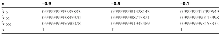
Table 3 Approximations atx= –0.9, –0.5, –0.1 foru(x) –₂1_π_–11 u(y)

(y–x)2dy=f(x)

x –0.9 –0.5 –0.1

ˆ

u10 0.999999993535333 0.999999981428145 0.999999917999549

ˆ

u100 0.999999993845970 0.999999988715871 0.999999990115998

ˆ

u1000 0.999999995690078 0.999999991935489 0.999999993153335

(9)

Table 4 Approximations atx= 0.1, 0.5, 0.9 foru(x) –₂1_π_–11 u(y)

(y–x)2dy=f(x)

x 0.1 0.5 0.9

ˆ

u10 0.999999917999549 0.999999981428145 0.999999993535332

ˆ

u100 0.999999990036579 0.999999988582430 0.999999992194477

ˆ

u1000 0.999999993375294 0.999999992061794 0.999999995726361

u 1 1 1

Table 5 Approximations atx= –0.9, –0.5, –0.1 foru(x) –_–11 ₍_yu(_–y_x)₎dy=f(x)

x –0.9 –0.5 –0.1

ˆ

u10 –1.194519628297830 –0.601189820467772 –0.156767445549832

ˆ

u100 –0.902665658196492 –0.496591018161909 –0.094652542268498

ˆ

u1000 –0.900369341742219 –0.499656299326138 –0.099458627117756

u –0.9 –0.5 –0.1

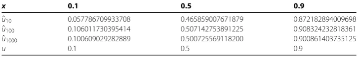
Table 6 Approximations atx= 0.1, 0.5, 0.9 foru(x) –_–11 u(y)

(y–x)dy=f(x)

x 0.1 0.5 0.9

ˆ

u10 0.057786709933708 0.465859007671879 0.872182894009698

ˆ

u100 0.106011730395414 0.507142753891225 0.908324232818361

ˆ

u1000 0.100609029282889 0.500725569118200 0.900861403735125

u 0.1 0.5 0.9

Example . Let us consider

u(x) –



– u(y)

(y–x)dy=f(x), |x|< ,

where

f(x) =x– –xln(x+ ) +xln( –x),

then

u(x) =x,

is the exact solution of equation.

Tables - also show that the proposed method is eﬀective and the convergence order isO(/N), which coincides with the classical theory of collocation methods.

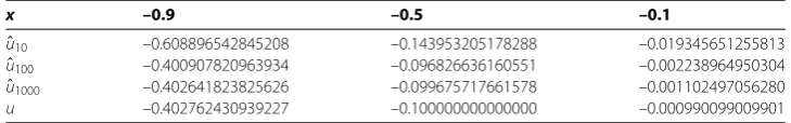
Example . For the more general case, we consider

u(x) +x– +x 

– u(y)

(y–x)dy=f(x), |x|< ,

where

f(x) =x–

 –π  + x

(10)

Table 7 Approximations atx= –0.9, –0.5, –0.1 foru(x) –_–11 ₍_yu(_–y_x)₎dy=f(x)

x –0.9 –0.5 –0.1

ˆ

u10 –0.608896542845208 –0.143953205178288 –0.019345651255813

ˆ

u100 –0.400907820963934 –0.096826636160551 –0.002238964950304

ˆ

u1000 –0.402641823825626 –0.099675717661578 –0.001102497056280

u –0.402762430939227 –0.100000000000000 –0.000990099009901

Table 8 Approximations atx= 0.1, 0.5, 0.9 foru(x) –_–11 ₍u_y(_–y_x)₎dy=f(x)

x 0.1 0.5 0.9

ˆ

u10 –0.025111748216482 0.052110055810136 0.363240467300408

ˆ

u100 –0.001202605523378 0.101502077326766 0.409787561038363

ˆ

u1000 0.000783503911385 0.100161733460852 0.403492522553747

u 0.000990099009901 0.1 0.402762430939227

and the exact solution is

u(x) = x



 +x.

Tables - also illustrate the eﬃciency and accuracy of the methods.

5 Conclusion

In this paper, we explore collocation methods for a singular Fredholm integral equation of the second kind and utilize the FMM to improve the eﬃciency of algorithm. Based on the multipole expansion of kernel, we demonstrate that the approximate operator used in the collocation equation converges to the initial operator. Numerical examples demonstrate the performance of the proposed algorithm.

Competing interests

The authors declare that they have no competing interests.

Authors’ contributions

All authors derived the proof. All authors conceived of the study and participated in its design and coordination. All authors read and approved the ﬁnal manuscript.

Author details

1_{Department of Mathematics and Computational Science, Hunan University of Science and Engineering, Yongzhou,}

425100, P.R. China.2_{School of Mathematics and Statistics, Central South University, Düsternbrooker Weg 20, Changsha,}

410083, P.R. China.

Acknowledgements

The authors are grateful to the anonymous referees for their constructive comments and helpful suggestions to improve this paper greatly. This work is supported by the Scientiﬁc Research Foundation of Education Bureau of Hunan Province under grant 14C0495, the Natural Science Foundation of Hunan Province of China under grant 14JJ3134, the NSF of China under grant 11371376, the Mathematics and Interdisciplinary Sciences Project of Central South University.

Received: 5 December 2014 Accepted: 21 May 2015 References

1. Kythe, PK, Puri, P: Computational Methods for Linear Integral Equations. Birkhauser, Boston (2002)

2. Junghanns, P, Kaiser, R: Collocation for Cauchy singular integral equations. Linear Algebra Appl.439, 729-770 (2013) 3. Venturino, E: The Galerkin method for singular integral equations revisited. J. Comput. Appl. Math.40, 91-103 (1992) 4. Gong, Y: Galerkin solution of a singular integral equation with constant coeﬃcients. J. Comput. Appl. Math.230,

393-399 (2009)

5. Bonis, MCD, Laurita, C: Numerical solution of systems of Cauchy singular integral equations with constant coeﬃcients. Appl. Math. Comput.219, 1391-1410 (2012)

(11)

7. Akel, MS, Hussein, HS: Numerical treatment of solving singular integral equations by using sinc approximations. Appl. Math. Comput.218, 3565-3573 (2011)

8. Mikhlin, SG, Prössdorf, S: Singular Integral Operators. Akademie, Berlin (1986)

9. Prössdorf, S, Silbermann, B: Numerical Analysis of Integral and Related Operator Equations. Akademie, Berlin (1991) 10. Graham, IG: Galerkin methods for second kind integral equations with singularities. Math. Comput.39, 519-533

(1982)

11. Herman, JJ, Riele, T: Collocation methods for weakly singular second-kind Volterra integral equations with non-smooth solution. IMA J. Numer. Anal.2, 437-449 (1982)

12. Xiang, S, He, K: On the implementation of discontinuous Galerkin methods for Volterra integral equations with highly oscillatory Bessel kernels. Appl. Math. Comput.219, 4884-4891 (2013)

13. Xiang, S, Brunner, H: Eﬃcient methods for Volterra integral equations with highly oscillatory Bessel kernels. J. Comput. Phys.53, 241-263 (2013)

14. Xiang, S, Wu, Q: Numerical solutions to Volterra integral equations of the second kind with oscillatory trigonometric kernels. Appl. Math. Comput.223, 34-44 (2013)

15. Wu, Q: On graded meshes for weakly singular Volterra integral equations with oscillatory trigonometric kernels. J. Comput. Appl. Math.263, 370-376 (2014)

16. Atkinson, KE: The Numerical Solution of Integral Equations of the Second Kind. Cambridge University Press, Cambridge (1997)

17. Golberg, MA: Numerical Solution of Integral Equations. Plenum Press, New York (1990)

18. Rokhlin, V: Rapid solution of integral equations of classical potential theory. J. Comput. Phys.60, 187-207 (1985) 19. Greengard, L, Rokhlin, V: A fast algorithm for particle simulations. J. Comput. Phys.73, 325-348 (1987)

20. Liu, YJ: Fast Multipole Boundary Element Method: Theory and Applications in Engineering. Cambridge University Press, Cambridge (2009)

21. Brunner, H: Collocation Methods for Volterra Integral and Related Functional Equations. Cambridge University Press, Cambridge (2004)

22. Abramowitz, M, Stegun, IA: Handbook of Mathematical Functions. National Bureau of Standards, Washington (1964) 23. Kress, R: Linear Integral Equation. Springer, Berlin (1999)