R E S E A R C H
Open Access
Stability of sets of stochastic functional
differential equations with impulse effect
Yan Xu and Zhimin He
**Correspondence:
[email protected] School of Mathematics and Statistics, Central South University, Changsha, Hunan 410083, People’s Republic of China
Abstract
In this paper, we study the stability of sets for a class of impulsive stochastic functional differential equations. By employing piecewise continuous Lyapunov functions with Razumikhin methods, some sufficient conditions are established to guarantee the stability of sets of impulsive stochastic functional differential equations and we also show that the impulses play an important role in the stability of stochastic functional differential equations. Three examples are presented to illustrate the effectiveness of the results obtained.
MSC: 34K20; 34K45; 34K50
Keywords: stability of sets; Brownian motion; stochastic functional differential equations; impulse; Lyapunov function; Razumikhin methods
1 Introduction
During the past few decades, the stability theory of stochastic differential equations and impulsive differential equations has been developed very quickly; see for instance [–]. A lot of stability criteria on impulsive stochastic differential equations have also been re-ported (see [–] and the references therein). Almost all of them mainly focus on the stability of the zero solution, but there is very little of research addressing the stability of sets.
The concept of stability of sets of nonlinear systems, which includes as a special case stability in the sense of Lyapunov (see Krasovskii []; Roucheet al.[]), such as stability of the trivial solution, stability of the solution, stability with respect to part of the vari-ables and so on, has become one of the most important issues in the stability theory of nonlinear systems [–]. The theoretical works of the stability of sets with respect to nonlinear ordinary differential equations may be traced back to Yoshizawa [–] in the previous century. The research to the stability of sets of impulsive differential equations can be found in [, –]. For stochastic differential equations and impulsive stochastic differential equations, we refer the reader to [, –] and the references therein.
In this paper, we shall extend the Razumikhin method developed in [, , ] to investi-gate the stability of sets for a class of impulsive stochastic functional differential equations. Meanwhile, our results show that the impulsive effects play an important part in the sta-bility for stochastic functional differential equations, that is, an unstable stochastic delay system can be successfully stabilized by impulses.
The rest of this paper is organized as follows. Some preliminary notes are given in Sec-tion . Several theorems on stability of sets of impulsive stochastic funcSec-tional differential equation are established in Section . In Section , three examples are presented to illus-trate the applications of the results obtained.
2 Preliminaries
Throughout this paper, we use the following notations.
Let (,F,{Ft}t≥,P) be a complete probability space with a natural filtration{Ft}t≥
sat-isfying the usual conditions (i.e.it is right continuous andFcontains allP-null sets), and
E[·] stand for the correspondent expectation operator with respect to the given probability measureP. LetW(t) = (W(t), . . . ,Wm(t))Tbe anm-dimensional Wiener process defined
on a complete probability space with a natural filtration. Let|·|denote the Euclidean norm inRn.
Letτ > andPC([–τ, ];Rn) = {φ: [–τ, ]→Rn|φ(t) is continuous everywhere
ex-cept at the pointst=tk∈[t,∞),φ(tk+) andφ(t–k) exist withφ(tk+) =φ(tk)}with the norm
φ=sup–τ≤θ≤|φ(θ)|, whereφ(t+) andφ(t–) denote the right-hand and left-hand limits
of functionφ(t) att. DenotePCb
F([–τ, ];R
n) by the family of all bounded,F-measurable,PC([–τ, ];Rn
)-valued random variables. Forp> , denote byPCFpt([–τ, ];Rn) the family of allF t
-mea-surablePC([–τ, ];Rn)-valued random variablesφsuch thatEφp<∞.
In this paper, we shall consider the following impulsive stochastic functional differential equation:
⎧ ⎪ ⎨ ⎪ ⎩
dx(t) =f(t,xt)dt+g(t,xt)dW(t), t≥t,t=tk,
x(tk) =Ik(tk,x(tk–)), t=tk,k∈Z+,
xt(s) =ξ(s), s∈[–τ, ],
(.)
whereZ+is the set of all positive integers,ξ={ξ(s) : –τ ≤s≤} ∈PCFb([–τ, ];Rn),x(t) =
[x(t),x(t), . . . ,xn(t)]T, andxt ={x(t+θ) : –τ ≤θ≤},x(t–k) =limh→–x(tk+h),x(tk) =
limh→+x(tk+h),tk(k= , , . . .) are impulsive moments satisfying ≤t<t<· · ·<tk<
tk+<· · ·withlimk→+∞tk= +∞,x(tk) =x(t+k) –x(tk–) =x(tk) –x(t–k) represents the jump in
the statexattkwithIkdetermining the size of the jump.f : [t,∞)×PC([–τ, ];Rn)→Rn
andg: [t,∞)×PC([–τ, ];Rn)→Rn×mare Borel measurable, andIk∈C(R+×Rn,Rn).
Definition . AnRn-valued stochastic processx(t) is called a solution of the problem
(.) corresponding to initial valueσ, if
(i) x:[σ–τ,σ+β)for someβ( <β≤ ∞) is continuous for
t∈[σ–τ,σ+β)\{tk:k= , , . . .},x(t+k)andx(tk–)exist withx(tk+) =x(tk)for
tk∈[σ–τ,σ+β), and{xt}t≥tisFt-adapted;
(ii) {f(t,xt)} ∈L([t,∞];Rn)and{g(t,xt)} ∈L([t,∞];Rn×m);
(iii) x(t)satisfies (.).
We denote the solution of the initial problem (.) byx(t;σ,ξ), and we denote by [σ–
τ,σ+β) the maximal right interval in which the solutionx(t;σ,ξ) is defined.
LetM⊂[t–τ,∞)×Rn. We introduce the following notations:
M(t) =x∈Rn: (t,x)∈M, t∈[t–τ,∞);
where
dx,M(t) = inf
y∈M(t)E|x–y|
is the distance betweenxand the setM(t);
M(t,) =ϕ∈PC[–τ, ];Rn :dϕ,M(t) <,> , where
dϕ,M(t) = max
s∈[–τ,]d
ϕ(s),M(t+s) and ϕ∈PC[–τ, ];Rn .
We assume that the following conditions (H)-(H) are satisfied, so that the initial value
problem (.) has one unique solution.
(H) For allψ∈PC([–τ, ];Rn)andk∈Z+, the limits
lim
(t,ϕ)→(t–
k,ψ)
f(t,ϕ) =ftk–,ψ , lim
(t,ϕ)→(t–
k,ψ)
g(t,ϕ) =gtk–,ψ
exist.
(H) f andgsatisfy the locally Lipschitz condition inφon each compact set inPC([–τ, ];
Rn). More precisely, for everya∈[t,σ+β)and every compact setG∈PC([–τ, ];
Rn), there exists a constantL=L(a,G)such that
f(t,ϕ) –f(t,ψ)∨g(t,ϕ) –g(t,ψ)≤Lϕ–ψ,
whenevert∈[t,a)andϕ,ψ∈G.
(H) For anyρ> there exists <ρ≤ρ, such that
x∈M(t,ρ) implies that x+Ik(tk,x)∈M(t,ρ)
for allk∈Z+.
(H) f(t,xt),g(t,xt)∈PC([t,∞),Rn)forxt∈PC([σ–τ,∞),Rn).
For anyt≥tandκ≥, letPCκ={φ∈PC([–τ, ];Rn) :φ ≤κ}.
We shall say that condition (A) is fulfilled if the following conditions hold:
(A) for eacht∈[t,∞)the setM(t)is not empty;
(A) for any compact subsetFof[t,∞)×Rnthere exists a constantK> depending on Fsuch that if(t,x), (t,x)∈F, then the following inequality holds:
d
x,M(t) –dx,Mt ≤Kt–t;
(A) if for solutionx(t;σ,ξ)there existsh> satisfying
dx(t;σ,ξ),M(t,ρ) ≤h<∞ fort∈[σ,σ+β),
Definition . A functionV(t,x) : [t–τ,∞)×M(t,ρ)→R+belongs to the classν if
(B) Vis continuous on each of the set([t–τ,t]∪[tk–,tk))×M(t,ρ)for allx∈M(t,ρ)
and fork∈Z+, the limitlim
(t,y)→(tk–,x)V(t,y) =V(t–k,x)exists;
(B) V is locally Lipschitz inx∈M(t,ρ), V(t, ) = for (t,x)∈M and V(t,x) > for
(t,x) /∈M.
Definition . For eachV∈ν, we define the operatorLV fromR+×RntoRby LV(t,φ) =Vt(t,x) +Vx(t,x)f(t,φ)
+ trace
gT(t,φ)Vxx(t,x)g(t,φ)
,
where
Vt(t,x) =
∂V(t,x)
∂t ,
Vx(t,x) =
∂V(t,x)
∂x , . . . ,
∂V(t,x)
∂xn
,
Vxx(t,x) =
∂V(t,x)
∂xi∂xj
n×n
.
We shall give the definitions of stability of the setMwith respect to system (.).
Definition . The setMwith respect to the solution of system (.) is said to be:
(S) stable, if for anyσ≥t,α> , and> , there is aδ(σ,,α) > such thatξ∈PCα∩
M(σ,δ)implies thatx(t,σ,ξ)∈M(t,)fort≥σ; (S) uniformly stable, if theδin (S) is independent ofσ;
(S) asymptotically stable, if it is stable and for anyσ ≥tandα> , there exists aδ=
δ(σ,α)such thatξ∈PCα∩M(σ,δ)implies thatx(t,σ,ξ)→M(t)ast→ ∞;
(S) uniformly asymptotically stable, if it is uniformly stable, and for anyα> there exists aδ(α) > , such that for any> there is aT(,α,δ) > such thatσ≥tandξ ∈ PCα∩M(σ,δ)implies thatx(t,σ,ξ)∈M(t,)fort≥σ+T.
In order to obtain our results, we will use the following function classes:
K=u∈CR+,R+ :u() = ,u(s) is strictly increasing ins;
K=u∈CR+,R+ :u() = ,u(s) > fors> ;
K=
u∈CR+,R+ :u() = ,u(s) >sfors> ,u(s) is strictly increasing ins.
3 Main results
In this section, we present and prove our main results on uniform stability and asymptotic stability of the sets of system (.) by utilizing piecewise continuous Lyapunov functions with Razumickhin methods.
(i) a(d(x,M(t)))≤EV(t,x)≤b(d(x,M(t)))for all(t,x)∈[t–τ,∞)×M(t,ρ); (ii) ELV(t,x(t))≤η(t)c(EV(t,x(t))),t= tk,wheneverEV(t+s,x(t+s))≤P(EV(t,x(t)))
for–τ≤s≤,wherex(t)is any solution of system(.),andη: [t,∞)→R+is
locally integrable;
(iii) EV(tk,x+Ik(tk,x))≤P–(EV(tk–,x))for eachk∈Z+,and allx∈M(t,ρ),whereP–
is the inverse of the functionP; (iv) supk∈Z+{tk–tk–}<∞,and
μ
P–(μ)cds(s)–
tk
tk–η(s)ds> for allμ∈(,∞),k∈Z
+.
Then the set M is uniformly stable with respect to the solution of system(.).
Proof For any given> ,α> , without loss of generality, we assume that≤ρ. We can
chooseδ=δ(,α) > such thatP(b(δ)) <α() andδ<α. Fromb(δ) <P(b(δ)) <α() <b() we know thatδ<.
Forσ≥t,ξ∈PCα∩M(σ,δ), letx(t) =x(t;σ,ξ) be the solution of system (.), where
σ∈[tm–,tm) for somem∈Z+. Then, forσ–τ≤t≤σ, from condition (i) we have
adx(t),M(t) ≤EVt,x(t) ≤bdx(t),M(t) ≤b(δ)≤Pb(δ) <a(). (.)
From the above inequality, we obtaind(x(t),M(t)) <forσ–τ≤t≤σ.
Next, we will proved(x(t),M(t)) < fort∈[σ,σ +β). Suppose, on the contrary, that
d(x(t),M(t)) >for somet∈[σ,σ+β). Then letˆt=inf{σ≤t≤σ+β|d(x(t),M(t)) >}. Note thatd(x(σ),M(σ)) <, we see thattˆ>σ,d(x(t),M(t))≤≤ρ, fort∈[σ–τ,ˆt) and eitherd(x(ˆt),M(ˆt)) =ord(x(ˆt),M(ˆt)) >andˆt=tkfor somek.
In the latter case,d(x(tˆ),M(tˆ))≤ρ. From condition (H) we have
dx(tˆ),M(tˆ) =dx(tk),M(tk) =d
xt–k +Ik
tk,x
tk– ,M(tk) ≤ρ,
it follows that in either caseEV(t,x(t)) is defined fort∈[σ–τ,tˆ]. Fort∈[σ,ˆt] define
EV(t) =EVt,x(t) . (.)
Then fort∈[σ–τ,ˆt], by condition (i), we get
adx(t),M(t) ≤EV(t)≤bdx(t),M(t) .
Let˜t=inf{t∈[σ,ˆt]|EV(t) >a()}. SinceEV(σ) <a() andEV(˜t)≥a(), it follows that
˜
t∈(σ,tˆ] andEV(t) <a() fort∈[σ–τ,˜t). We claim thatEV(˜t) =a() and that˜t=tkfor
anyk. In fact, ifEV(˜t)≥a(),t˜=tkfor somek, by condition (iii) we have
a()≤EV(˜t)≤P–EVt˜– <EV˜t– ≤a(),
which is contradiction. Thus˜t=tk, for anyk, and that in turn impliesEV(˜t) =a(), since
EV(t) is continuous at˜tfor˜t=tk.
Now let us first consider the casetm–≤ ˜t<tm. Lett¯=sup{t∈[σ,˜t]|EV(t)≤P–(a())}.
Fort∈[¯t,˜t] and –τ ≤s≤, we have
EV(t+s)≤a() =PP–a() ≤PEV(t).
From condition (ii), we obtain
ELV(t)≤η(t)cEV(t)
for allt∈[¯t,t˜]. Integrating the above differential inequality yields
EV(˜t)
EV(¯t) ds c(s)≤
˜t
¯
t
η(s)ds≤ tm
tm–
η(s)ds. (.)
On the other hand, by condition (iv), we obtain
EV(˜t)
EV(¯t) ds c(s)=
a()
P–(a())
ds c(s)>
tm
tm–
η(s)ds,
which is in contradiction with (.).
Now, assume thattk<t˜<tk+ for somek∈Z+ andk≥m. Then by condition (iii) we
have
EV(tk)≤P–
EVt–k <P–a() .
Let¯t=sup{t∈[tk,˜t]|EV(t)≤P–(a())}. Thent¯∈(tk,˜t),EV(t¯) =P–(a()), andEV(t)≥
P–(a()) fort∈[¯t,˜t]. Therefore, fort∈[t¯,˜t] and –τ≤s≤, we have
EV(t+s)≤a() =PP–a() ≤PEV(t).
Then, by condition (ii), we have
ELV(t)≤η(t)cEV(t) for allt∈[¯t,˜t].
Integrating the above differential inequality yields
EV(˜t)
EV(¯t) ds c(s)≤
˜t
¯
t
η(s)ds≤ tk+
tk
η(s)ds. (.)
On the other hand, by condition (iv), we have
EV(˜t)
EV(¯t) ds c(s)=
a()
P–(a())
ds c(s)>
tk+
tk
η(s)ds,
which is in contradiction with (.). So in either case, we get a contradiction, so we obtain
From condition (A) we know that [σ,σ+β) = [σ,∞), hencex(t)∈M(t,), for allt≥σ,
which implies that the setMis uniformly stable with respect to the solution of system
(.). The proof of Theorem . is complete.
Remark . From Theorem ., we know that impulsive perturbations may cause uniform stability even if the unperturbed system is unstable.
The following result on the asymptotical stability of sets will reveal that impulsive per-turbation make stable systems asymptotically stable.
Theorem . Let conditions(A)and(H)-(H)be satisfied and suppose that there exist functions V ∈ν,a,b∈K,hk∈C(R+,R+)for k∈Z+,and the following conditions are
fulfilled:
(i) a(d(x,M(t)))≤EV(t,x)≤b(d(x,M(t)))for all(t,x)∈[t–τ,∞)×M(t,ρ); (ii) EV(tk,x+Ik(tk,x)) –EV(tk–,x)≤–hk(EV(t–k,x))for allk∈Z+andx∈M(t,ρ); (iii) for any solutionx(t)of system(.),ELV(t,x)≤;,and for anyσ≥t,andr> ,
there exists{rk}such thatEV(t,x)≥rfort≥σ implies thathk(EV(tk–,x))≥rk;
whererk≥with
∞
k=rk=∞.
Then the set M with respect to the solution of system(.)is uniformly stable and asymp-totically stable.
Proof At first, we show that the setMis uniform stability.
For given> (≤ρ),α> , we choose aδ(,α) > such thatb(δ)≤a() andδ<α.
For anyσ≥tandξ∈PCα∩M(σ,δ), letx(t) =x(t;σ,ξ) be the solution of system (.).
We will show thatx(t)∈M(t,) fort∈[σ,σ+β).
SetEV(t) =EV(t,x(t)), whereσ∈[tm–,tm) for somem∈Z+. Then condition (iii)
im-plies thatELV(t)≤ fort∈[σ,σ+β)∩([σ,tm)∪(∞k=m[tk–,tk))),k∈Z+.
By condition (ii) we haveEV(ti) –EV(ti–)≤ for allσ≤ti≤σ+β. ThusEV(t) is
non-increasing on [σ,σ+β). From condition (i) it follows that
adx(t),M(t) ≤EV(t)≤EV(σ)≤b(δ)≤a()
forσ≤t≤σ+β. From condition (A) we obtain [σ,σ+β) = [σ,∞). Sinced(x(t),M(t))≤ , for allt≥σ, this implies thatx(t)∈M(t,) fort≥σ. That is, the setMis uniformly stable with respect to the solution of system (.).
Next we shall prove that the setMis asymptotically stable.
From conditions (ii), (iii), andEV(t)≥, we note thatEV(t) is non-increasing on the interval [σ,∞). So the limitlimt→∞EV(t) exists.
Assumeσ∈[tm–,tm] for somem∈Z+. Setlimt→∞EV(t) =r≥, one can easily see that
EV(t)≥rfort≥σ. Then by condition (iii), it follows that there is a sequence{rk}with
rk≥ fork∈Z+, which implies thathk(EV(tk–,x))≥rkwith∞k=rk=∞.
By conditions (ii) and (iii) we get
EV(t)≤EV(σ) +
σ≤tk≤t
EV(tk) –EV
tk– ≤EV(σ) –
σ≤tk≤t hk
EVt–k ≤EV(σ) –
σ≤tk≤t
which is a contradiction. Hence we haver= , which implies thata(d(x,M(t)))→ as
t→ ∞. That is,x(t)→M(t) ast→ ∞. The proof of Theorem . is complete.
Theorem . Let conditions(A)and(H)-(H)be satisfied and suppose that there exist functions V∈ν,a,b∈K,ψk,C∈K,and the following conditions are fulfilled:
(i) a(d(x,M(t)))≤EV(t,x)≤b(d(x,M(t)))for all(t,x)∈[t–τ,∞)×M(t,ρ); (ii) EV(tk,x+Ik(tk,x))≤ψk(EV(t–k,x)),for allK∈Z+,andx∈M(t,ρ);
(iii) for any solutionx(t)of system(.),ELV(t,x)≤–θ(t)C(EV(t,x))fort=tk,where
θ: [t,∞)→R+is locally intergrade,and there existsμ,such that for any μ∈(,μ),
ψk(μ)
μ
ds C(s)–
tk
tk–
θ(s)ds≤–γk,
whereγk≥with
∞
k=γk=∞.
Then the set M with respect to the solution of system(.)is uniformly stable and asymp-totically stable.
Proof Without loss of generality, for any given> ,α> , we can assume that≤ρ. We
choose aβ: <β<min{a(),μ}such thatψk(s) <a() for ≤s≤βand for allk∈Z+.
Setδ=δ(,α) > be such thatb(δ) <β andδ<α. Letx(t) =x(t;σ,ξ) be the solution of system (.), whereσ≥tandξ∈PCα∩M(σ,δ). At first, we show that
x(t)∈M(t,) fort∈[σ,σ+β). (.)
SetEV(t) =EV(t,x(t)) andσ∈[tm–,tm) for somem∈Z+.
By condition (iii), we getELV(t,x)≤ forσ≤t<tm. It follows that
EV(t)≤EV(σ)≤b(δ) <β<a()
forσ ≤t<tm. So forσ ≤t<tm, we havex(t)∈M(t,). Thus if (.) is not true, then
there exists a¯t∈[tk,tk+) for somek∈Z+,k≥msuch thatx(t)∈M(t,) forσ≤t<¯t, and x(¯t) /∈M(¯t,). Using conditions (ii) and (iii), we have, fori=m,m+ , . . . ,k– ,
ELV(t)≤–θ(t)CEV(t) , ti≤t<ti+ (.)
and
EV(ti)≤ψi
EVt–i . (.)
So by (.), we have
EV(tm)≤ψm
EVt–m ≤ψm
b(δ) <a(). (.)
From (.) and (.), fori=m,m+ , . . . ,k– , we have
EV(ti–+)
EV(ti) ds C(s)≤–
ti+
ti
and
EV(ti+)
EV(t–
i+)
ds C(s)≤
ψ(EV(t–
i+))
EV(t–
i+)
ds
C(s). (.)
Thus by (.) and condition (iii), we obtain
EV(ti+)
EV(ti) ds C(s)≤
ψ(EV(t–i+))
EV(t–i+) ds C(s)–
ti+
ti
θ(s)ds≤–γi+, (.)
which impliesEV(ti+)≤EV(ti) fori=m,m+ , . . . ,k– . From this and (.) we have
EV(tk)≤ · · · ≤EV(m) <a(). (.)
But by condition (i), we havea()≤a(d(x(¯t),M(t¯)))≤EV(¯t)≤EV(tk) <a(), which is a
contradiction. Thus (.) holds, from condition (A) it follows that (σ–τ,σ+β) = (σ– τ,∞), hencex(t)∈M(t,), for allt≥. So the setMis uniformly stable with respect to the solution of system (.).
To prove the asymptotically stability, we observe that, from the proof of (.), one finds thatEV(ti+)≤EV(ti) holds for alli≥m. Thus we havelimt→∞EV(ti) =αexists andα≥.
Ifα> , (.) yields
EV(ti+)
EV(ti) ds
C(s)≤–γi+, i=m,m+ , . . . . (.)
Let¯c=infα≤s<a()C(s). From (.), we get
EV(ti+)≤EV(ti) –cγ¯ i+, i=m,m+ , . . . , (.)
which implies
EV(tk)≤EV(tm) –c¯ k–
i=m
γi+→–∞
ask→ ∞. It is a contradiction and soα= .
SinceEV(t)≤EV(tk) fortk≤t<tk+, it follows that limt→∞EV(t) = , which yields
limt→∞d(x(t,M(t))) = . The proof of Theorem . is complete. 4 Illustrative examples
As an application, we consider the following examples.
Example . Consider the scalar impulsive stochastic delay differential equation:
dx(t) = (–x(t) + .x(t–τ))dt+√
x(t–τ)dW(t), t=tk, x(tk) = .x(t–k), k= , , . . . ,
(.)
whereτ > ,t<t<t<· · ·<tk→ ∞ask→ ∞. Assume that the following condition is
satisfied:
LetM(t) ={(t, ) :t∈[t–τ,∞)},V(t,x) =V(x) = .x,P(s) = s,c(s) =s, then
EVx+Ik(tk,x) =EV(.x) =E
.x =P–EV(x) ,
and for any solutionx(t) of system (.), such that
EVt+s,x(t+s) ≤PEVx(t) , –τ≤s≤,t≥t.
Clearly, we haveEx(t–τ)≤Ex(t),t≥t
. Hence,
ELVx(t) = –Ex(t) + .Ex(t)x(t–τ) + .×.Ex(t–τ)
≤–Ex(t) + .Ex(t) + .Ex(t)
=η(t)cEVx(t) ,
whereη(t) = . > . We have
tk–tk–< –
ln. .
and for anyμ> ,k∈Z+,
μ
P–(μ)
ds c(s)–
tk
tk–
η(s)ds=
μ
hμ
ds c(s)–
tk
tk–
η(s)ds
> –ln. –
–ln. .
××(.)
= .
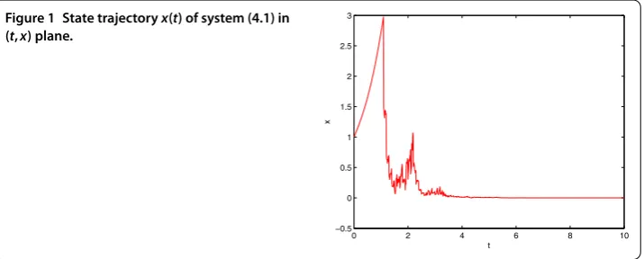
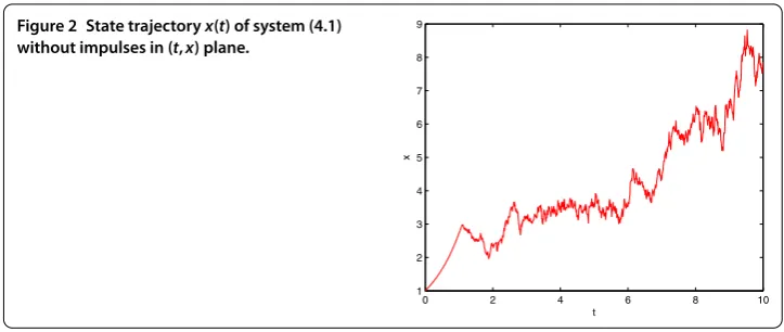
Thus all of the conditions in Theorem . are satisfied. Therefore, it follows from The-orem . that the set Mis uniformly stable with respect to the solution of the system (.). The simulation result of system (.) is shown in Figure . The simulation of system (.) without impulses is shown in Figure . From Figures and , we find that, although stochastic delay differential equations without impulse may be unstable, adding impulses may lead to stability. That is, impulsive perturbations play an important role in the stability behavior of nonlinear systems.
Figure 2 State trajectoryx(t) of system (4.1) without impulses in (t,x) plane.
Example . Consider the scalar impulsive stochastic delay differential equation:
orem . are satisfied. Therefore, it follows from Theorem . that the setMis uniformly stable and asymptotically stable with respect to the solution of the system (.).
Example . Consider the scalar impulsive stochastic delay differential equation:
dx(t) = (ax(t) +bx(t–τ))dt+ (cx(t) +rx(t–τ))dW(t), t=tk,
x(tk) =hx(tk–), k= , , . . . ,
whereτ> ,t<t<t<· · ·<tk→ ∞ask→ ∞. Assume that the following conditions
rem . are satisfied. Therefore, it follows from Theorem . that the setMis uniformly stable and asymptotically stable with respect to the solution of the system (.).
Competing interests
The authors declare that they have no competing interests.
Authors’ contributions
All authors contributed equally to the writing of this paper. All authors read and approved the final manuscript.
Acknowledgements
The authors would like to thank the referee for his/her careful reading and valuable suggestions, which lead to improvement of the manuscript.
References
1. Bao, JH, Hou, ZT, Yuan, CG: Stability in distribution of mild solutions to stochastic partial differential equations. Proc. Am. Math. Soc.138, 2169-2180 (2010)
2. Bao, JH, Truman, A, Yuan, CG: Stability in distribution of mild solutions to stochastic partial differential delay equations with jumps. Proc. R. Soc. Lond. Ser. A465, 2111-2134 (2009)
3. Bao, JH, Hou, ZT, Yuan, CG: Stability in distribution of neutral stochastic differential delay equations with Markovian switching. Stat. Probab. Lett.79, 1663-1673 (2009)
4. Khasminskii, R: Stochastic Stability of Differential Equations, 2nd edn. Springer, Berlin (2012) 5. Ladde, GS, Lakshmikantham, V: Random Differential Inequalities. Academic Press, New York (1980)
6. Ladde, GS, Sambandham, M: Stochastic versus Deterministic Systems of Differential Equations. Dekker, New York (2004)
7. Lakshmikantham, V, Bainov, DD, Simeonov, DS: Theory of Impulsive Differential Equation. World Scientific, Singapore (1989)
8. Lakshmikantham, V, Liu, X: Stability of impulsive differential systems in terms of two measures. Appl. Math. Comput.
29, 89-98 (1989)
9. Liu, X, Wang, Q: On stability in terms of two measures for impulsive systems of functional differential equations. J. Math. Anal. Appl.326, 252-265 (2007)
10. Mao, X: Stochastic Differential Equations and Their Applications, 2nd edn. Horwood, Chichester (2007) 11. Mao, X: Attraction, stability and boundedness for stochastic differential delay equations. Nonlinear Anal.47,
4795-4806 (2001)
12. Samoilenko, AM, Perestyuk, NA: Impulsive Differential Equations. World Scientific, Singapore (1995)
13. Shaikhet, L: Lyapunov Functionals and Stability of Stochastic Functional Differential Equations. Springer, New York (2013)
14. Shen, J, Yan, J: Razumikhin type stability theorems for impulsive functional differential equations. Nonlinear Anal.33, 519-531 (1998)
15. Stamova, I: Stability Analysis of Impulsive Functional Differential Equations. de Gruyter, New York (2009) 16. Caro, EA, Rao, ANV: Stability analysis of impulsive stochastic differential systems in terms of two measures. In:
Conference Proceedings COM, pp. 132-135. IEEE Press, New York (1996)
17. Pan, L, Cao, J: Exponential stability of impulsive stochastic functional differential equations. J. Math. Anal. Appl.382, 672-685 (2011)
18. Liu, J, Liu, X, Xie, W: Impulsive stabilization of stochastic functional differential equations. Appl. Math. Lett.24, 264-269 (2011)
19. Liu, ZM, Peng, J:p-Moment stability of stochastic nonlinear delay systems with impulsive jump and Markovian switching. Stoch. Anal. Appl.27, 911-923 (2009)
20. Peng, S, Jia, B: Some criteria onpth moment stability of impulsive stochastic functional differential equations. Stat. Probab. Lett.80, 1085-1092 (2010)
21. Rao, ANV, Tsokos, CP: Stability behavior of impulse stochastic differential systems. Dyn. Syst. Appl.4, 317-327 (1995) 22. Zhang, S, Sun, J, Zhang, Y: Stability of impulsive stochastic differential equations in terms of two measures via
perturbing Lyapunov functions. Appl. Math. Comput.218, 5181-5186 (2012)
23. Xu, Y, He, ZM: Stability of impulsive stochastic differential equations with Markovian switching. Appl. Math. Lett.35, 35-40 (2014)
24. Krasovskii, NN: Stability of Motion. Stanford University Press, Stanford (1963)
25. Rouche, H, Habets, P, Laloy, M: Stability Theory by Lyapunov’s Direct Method. Springer, New York (1977) 26. Lakshmikantham, V, Leela, S, Martynyuk, AA: Stability Analysis of Nonlinear Systems. Dekker, New York (1989) 27. Lakshmikantham, V, Leela, S, Martynyuk, AA: Practical Stability Analysis of Nonlinear Systems. World Scientific,
Singapore (1990)
28. Lakshmikantham, V, Liu, X: Stability Analysis in Terms of Two Measures. World Scientific, Singapore (1993) 29. Yoshizawa, T: Stability of sets and perturbed system. Funkc. Ekvacioj5, 31-69 (1962)
30. Yoshizawa, T: Some notes on stability of sets and perturbed system. Funkc. Ekvacioj6, 1-11 (1964)
31. Yoshizawa, T: Stability Theory by Lyapunov’s Second Method. The Mathematical Society of Japan, Tokyo (1966) 32. Kulev, GK, Bainov, DD: Stability of sets for impulsive systems. Int. J. Theor. Phys.28(2), 195-207 (1989)
33. Kulev, GK, Bainov, DD: Global stability of sets for impulsive differential systems by Lyapunov’s direct method. Comput. Math. Appl.19, 17-28 (1990)
34. Xie, S: Stability of sets of functional differential equations with impulse effect. Appl. Math. Comput.218, 592-597 (2011)
35. Xie, S, Shen, J: Stability of sets for impulsive functional differential equations via Razumikhin method. J. Math. Sci.177, 474-486 (2011)
36. Long, S: Attracting and invariant sets of nonlinear stochastic neutral differential equations with delays. Results Math.
63, 745-762 (2013)
37. Samoilenko, AM, Stanzhytskyi, O: Qualitative and Asymptotic Analysis of Differential Equations with Random Perturbations. World Scientific, Singapore (2011)
38. Luo, JW: Stability of invariant sets of Itô stochastic differential equations with Markovian switching. J. Appl. Math. Stoch. Anal.2006, Article ID 59032 (2006)
39. Xu, LG, Xu, DY:P-Attracting andp-invariant sets for a class of impulsive stochastic functional differential equations. Comput. Math. Appl.57, 54-61 (2009)