Performance Analysis of a Cluster Based MAC Protocol for Wireless Ad Hoc Networks

(1)

Volume 2010, Article ID 625619,16pages doi:10.1155/2010/625619

Research Article

Performance Analysis of a Cluster-Based MAC Protocol for

Wireless Ad Hoc Networks

Jes ´us Alonso-Z´arate,

1

_{Elli Kartsakli,}

2

_{Luis Alonso,}

2

_{and Christos Verikoukis}

1

1_{Access Technologies Area, Telecommunications Technology Center of Catalonia (CTTC), 08860 Castelldefels, Spain}

2_{Department of Signal Theory and Communications, The Technical University of Catalonia (UPC), 08860 Castelldefels, Spain}

Correspondence should be addressed to Jes ´us Alonso-Z´arate,[email protected]

Received 6 November 2009; Accepted 30 March 2010

Academic Editor: Xinbing Wang

Copyright © 2010 Jes ´us Alonso-Z´arate et al. This is an open access article distributed under the Creative Commons Attribution License, which permits unrestricted use, distribution, and reproduction in any medium, provided the original work is properly cited.

An analytical model to evaluate the non-saturated performance of the Distributed Queuing Medium Access Control Protocol for Ad Hoc Networks (DQMANs) in single-hop networks is presented in this paper. DQMAN is comprised of a spontaneous, temporary, and dynamic clustering mechanism integrated with a near-optimum distributed queuing Medium Access Control (MAC) protocol. Clustering is executed in a distributed manner using a mechanism inspired by the Distributed Coordination Function (DCF) of the IEEE 802.11. Once a station seizes the channel, it becomes the temporary clusterhead of a spontaneous cluster and it coordinates the peer-to-peer communications between the clustermembers. Within each cluster, a near-optimum distributed queuing MAC protocol is executed. The theoretical performance analysis of DQMAN in single-hop networks under non-saturation conditions is presented in this paper. The approach integrates the analysis of the clustering mechanism into the MAC layer model. Up to the knowledge of the authors, this approach is novel in the literature. In addition, the performance of an ad hoc network using DQMAN is compared to that obtained when using the DCF of the IEEE 802.11, as a benchmark reference.

1. Introduction

The IEEE 802.11 Standard for Wireless Local Area Networks (WLANs) defines both the physical (PHY) and the Medium Access Control (MAC) layer specifications [1]. Since its first release version in 1999, several amendments (referred to as the extensionsa, b,g,e, orn, among others) have been added to the standard, incorporating more sophisticated PHY layer schemes to attain higher performance in WLAN. However, the foundations of the MAC protocol have survived across the evolution of the standard. Despite few modifications, for example, the 802.11e to provide Quality of Service, its operation remains almost unaltered. Unfortunately, as data transmission rates grow, the MAC protocol overhead is becoming a bottleneck for the performance of next generation wireless networks [2]. For this reason, it is necessary to develop new protocols with reduced overhead that can attain higher performance.

This was the main motivation for the design of the Distributed Queuing MAC protocol for Ad Hoc Networks

(2)

However, saturation conditions only represent partially the performance of a practical network, which will not be working at the saturation point continuously. This is the motivation for this paper, where we present a novel theoretical model of DQMAN to evaluate its performance in non-saturation conditions for single-hop networks. With this model we derive the non-saturation throughput, the average transmission delay, and the average time that each node operates in the diﬀerent modes of operation in a DQMAN network. This last calculation is very important in energy-constrained networks in order to optimize the clustering algorithm from an energetic point of view. It is worth mentioning that this paper focuses on single-hop networks, while the simulation-based performance evaluation of DQMAN in multihop settings was presented in [6] and its theoretical analysis remains an open topic for future research.

The remainder of the paper is organized as follows. A description of DQMAN is presented inSection 2.Section 3 is dedicated to the description of the analytical model. In

Section 4, we use the model to evaluate the performance

of a DQMAN network in terms of throughput, delay, and clustering metrics. Then, the model is validated inSection 5 by comparing the theoretical results with those obtained via computer simulations. Then, the performance of DQMAN is compared to that of the IEEE 802.11 MAC protocol in

Section 6, demonstrating the suitability of DQMAN to be

considered for implementation in next generation wireless networks. Finally,Section 7concludes the paper and outlines future lines for research.

2. DQMAN Overview

DQMAN has been designed as a layer-2 mechanism for wire-less ad hoc networks where a number of users are equipped with half-duplex radio stations and share a single common radio channel with any arbitrary bandwidth. The key idea behind DQMAN is that whenever a station seizes the channel to transmit its data packets by executing a distributed access mechanism similar to that of the Distributed Coordination Function (DCF) of the IEEE 802.11 Standard [1], it estab-lishes a temporary one-hop cluster structure. The station which successfully seizes the channel becomes a temporary clusterhead and it coordinates the data transmissions of all the stations within its transmission range for a bounded period of time. The protocol running within each cluster is a variation of the near-optimum DQCA protocol for infrastructure-based WLANs [4] which, despite requiring the presence of a central point coordinator, operates in a completely distributed manner. The way the clustering algorithm is combined with an infrastructure-based protocol in DQMAN constitutes an innovative concept design within the context of MAC protocols for wireless ad hoc networks. It allows extending the ideas of DQCA to infrastructureless networks and it could be easily generalized to extend any other centralized MAC protocol to an infrastructureless network. Accordingly, the model presented in this paper could be easily extended to any other MAC protocol based

on the concept design of DQMAN. In the next sections, we review both the clustering algorithm and the MAC protocol of DQMAN.

2.1. Clustering Algorithm. Traditionally, clustering algo-rithms have been designed based on the idea that the more stable the cluster set, the better the network will perform [7–9]. The process of reclustering a part of the network may entail a high cost in terms of resources due to the fact that one clusterhead reassignment could trigger the re-configuration of the entire network. This could happen, for example, when the topology changes due to the mobility of the stations. This is known as the ripple effect of reclustering and it has been traditionally avoided, especially in the case of large mobile ad hoc networks. However, when mobility is present, cluster stability is difficult to attain. In addition, if some stations are to bea priorielected as clusterheads, it is difficult to design efficient criteria for selecting clusterheads in an extremely dynamic and changing environment as in the case of mobile wireless networks. As demonstrated in [10], the optimal clusterhead set problem is NP-complete, that is, it cannot be solved in polynomial time and, therefore, suboptimal clustering must be carried out in a dynamic environment. This is the main motivation for the passive, spontaneous, and dynamic clustering mechanism considered in DQMAN. Clusters are spontaneously created without explicit control information exchange whenever a station has data to transmit. The cluster structure is maintained for as long as there is data traffic pending to be transmitted among all the stations associated to a cluster. Therefore, the cluster structure is dynamically established and broken up according to the aggregate traffic load and the mobility of the network. Considering the clustering techniques compared and discussed in [8,11], and particularly the approach in [12], where the concept of passive clustering was first presented, the clustering algorithm of DQMAN was designed on the basis of the following:

(1) avoiding explicit clustering overhead,

(2) enabling future integration with legacy IEEE 802.11 networks, that is, backwards compatibility to a certain extent,

(3) sharing in a fair manner the responsibility of becom-ing clusterhead among all the stations of the network.

The clustering algorithm of DQMAN is based on a one-hop hierarchical master-slave architecture wherein any station can operate in one of the following three modes: master,slave, oridle. Any station should be able to switch from one mode of operation to another according to the dynamics of the network. For clarity of explanation, it will be used hereafter the single terms master and slave to denote stations operating in either master or slave mode. The terms stationandmodewill be dropped to clarify the discussion.

(3)

any knowledge of the cluster members of its cluster. This is a key feature of the overall mechanism as it minimizes the control load and facilitates its use in highly dynamic and unpredictable environments.

Despite the hierarchical master-slave cluster structure, all the communications are done in a peer-to-peer fashion between any pair of source and destination stations. Note that the term destination in this context refers to the next-hop destination of a packet (which will be specified by the routing protocol) and not necessarily to its final destination station. Routing is out of the scope of the basic definition of DQMAN, but any existing routing protocol could be applied on top of DQMAN without any restriction. Therefore, the master just acts as an indirect coordinator of the peer-to-peer communications within the cluster but ithas no explicit control on the access to the channel.

2.1.1. Cluster Formation and Maintenance. Any idle station with data to transmit initially listens to the channel for a deterministic period of time performing the so-called Clear Channel Assessment (CCA) in a similar way to the DCF of the IEEE 802.11 for data transmission. This sensing time is referred to as the Initial Master Sensing Interval (IMSI). It is worth mentioning that in the context of the standard, this IMSI corresponds to the initial Distributed Inter Frame Space (DIFS). If the channel is sensed idle for the entire IMSI, then the station attempts to establish a Master Service Set (MSS), which is actually an implicit cluster. The station becomes master and starts broadcasting a clustering beacon (CB) everyTframeseconds. For clarity in the explanation, it is considered that thisinterbeaconperiod has a constant duration, although it could have a variable duration depending on the packet sizes and the transmission rates.

The periodic transmission of the CBs defines a MAC frame structure and allows neighboring stations to get syn-chronized with the master (at the packet level) and to become implicit slaves. Slaves are responsible for transmitting an in-band busy tone (BT) upon the reception of each CB transmitted by the master. This MAC frame structure is illustrated inFigure 1. In this example, a station operating in master mode transmits a CB everyTframeseconds. Upon the reception of the CB, the two associated slave stationsiand j

transmit a BT. Finally, the time periods between BTs and CBs are used for the transmission of data packets.

The BTs promote a minimum distance of three hops between masters and allow combating the hidden terminal problem at the cost of exacerbating the exposed terminal problem. In addition, the BTs constitute a collision detection mechanism for those stations that attempt to become master. Note that if a recently set master does not sense any BT after the transmission of the CB, this is because there are no available slaves present in its neighborhood. Two situations may produce this fact.

(1) A collision has occurred with another station attempting to become master simultaneously.

(2) It constitutes an isolated master with no other station in its vicinity.

In the case of success, the time elapsed between the BTs and the next CB is devoted to the exchange of data and control packets. It is worth mentioning that in the case that all the stations of the network are in the transmission range of one another (no hidden terminals) the IMSI can take the duration of a DIFS, as in the 802.11 Standard. Otherwise, in general multihop settings with the potential presence of hidden terminals, this IMSI must take the value of the maximum time that an active master will remain silent, which corresponds to the time between two consecutive BTs. On the other hand, if an idle station senses the channel busy when attempting to get access to it for the first time or it collides when attempting to become master, it initiates a Master Selection Phase (MSP), that is, a random backoff time. This phase consists in setting up a Master Selection Silent Interval (MSSI) counter to a random value. This value must be within a MSSI window (measured in time slots) according to the algorithm presented in the next section. This operation is similar to the Binary Exponential Backoffof the IEEE 802.11 Standard, which uses the terms backoffcounter and Contention Window (CW), respectively. Likewise, any station performing an MSP listens to the channel and decrements the MSSI counter by one unit after each time slot as long as the channel is sensed idle. Upon the expiration of the MSSI counter, the station attempts to establish its MSS (cluster). The algorithm to set the initial value of the MSSI counter is presented in the following section.

2.1.2. Setting the MSSI. The MSSI selection algorithm is summarized as

MSSI=β+V, (1) where V = Uniform[0,α−1], that is, a uniform integer random variable between 0 andα−1, andβis a deterministic period of time. α ≥ 1 andβ ≥ 0 are tunable parameters that have integer values. The purpose of the fixed minimum period of timeβis to reduce the probability that a station becomes master twice consecutively in time, as it was shown in [3]. The randomized time intervalV reduces the probability that two or more stations attempt to become master simultaneously and collide. Since the parameter α

defines the size of the uniform random contention window, its value should be properly selected as a function of the number of active stations and the oﬀered load to the network. A proper tuning of this parameter avoids either unnecessary wasted time in deferral periods or a high probability of collisions. Despite this algorithm, collisions can still occur. The collision resolution algorithm of DQMAN is described in the next section.

(4)

Slavei

Slavej

Master CB MPDU CB CB

MAC frame BT BT

BT BT

BT MPDU BT

MPDU

· · · · · · · · ·

Time+ CB: clustering beacon broadcast by the master station

BT: busy tone transmitted by slave stations MPDU: MAC protocol data unit

Figure1: Clustering + MAC Structure.

receive them properly. The stations involved in the collision reinitiate a new MSP by selecting a new value for their respective MSSI counters as soon as the collision is detected.

2.1.4. Dynamic Reclustering. Any master reverts to idle whenever there are no more pending data transmissions among all the stations associated to its cluster (including its data traffic). A master can easily learn whether there is no data activity in the network using the MAC protocol rules and the state of the two distributed logical queues that manage both the collision resolution and the transmission of data (seeSection 2.2for an overview of the MAC protocol operation and [4] for the details of the protocol rules). Therefore, the cluster layout is dynamically changed along time as a function of the aggregated traffic load offered to the different sets of nodes in the network.

In addition, whenever a slave mishears a number of CBs from the master, it reverts to idle. Note that this happens if the master has either moved away from the slave (or vice versa) or the former has been switched oﬀ. It is worth mentioning that due to the channel fading and shadowing, a CB can be lost without implying that the connection with the master has been permanently lost. For these cases, it is convenient to consider that a master is not reachable if more than one CB is lost. Without loss of generality, and unless otherwise stated, it will be henceforth considered that a slave disassociates from the master if it mishears two consecutive CBs.

In addition, in order to avoid potential static cluster settings under heavy traﬃc conditions, any master reverts to idle after a bounded period of time regardless of the waiting data to be transmitted within its cluster. This is referred to as the Master Time Out (MTO) mechanism; any master decrements its MTO counter by one unit after the transmission of each CB, that is, after each MAC frame. Upon expiration of the counter, the station always reverts to idle mode regardless of the data activity of the network. The criteria to determine the value of this maximum time has been comprehensively studied in [13], showing a tradeoﬀ between fairness, in terms of sharing the responsibility of being master among all the users of the network, and maximum performance in terms of throughput.

2.2. The MAC Protocol. Within the context of DQMAN, the clustering beacon (CB) described before gets the form of a control packet, named Feedback Packet (FBP). This FBP

can be seen as the CB with additional control information necessary for the protocol operation. Therefore, the FBP is periodically broadcast by the master within each cluster, defining the time-frame structure depicted inFigure 2. All the stations within a cluster are synchronized with this time structure. Every frame is divided into three parts.

(1) A contention window (CW), further divided into m access minislots (typically 3 [5]) wherein slaves with data ready to transmit must send an Access Request Sequence (ARS).These sequences are pseudo-noise- (PN-) coded signals that allow the master station to decide whether each of the m minislots is in one out of three possible states: (i) empty, (ii) success, corresponding to the fact that just one ARS has been sent, or (iii) collision, when more than one (no matter how many) ARS have been sent within the same minislot. A mechanism to ensure the proper operation of the detection of the state of each minislot is the subject of a patent [14].

(2) A data part devoted to an almost collision-free transmission of data packets. The duration of this part depends on both the data transmission rate and the bit length of the data packets, which could change dynamically along time.

(3) A control part devoted to the exchange of the following control signaling:

(a) ACK packets sent by any destination station upon the reception of a data packet,

(b) the FBP broadcast by the master of the cluster. This packet contains the minimum control feedback information required to execute the rules of the protocol at each slave,

(c) in-band busy tones (BTs) transmitted by the slaves associated to a master. Since busy tones do not have to contain any information, they can be simple pseudo-random sequences, fol-lowing the same operation as the ARS.

(5)

Station 0: master _FBP

Contention window Slaves with data packets ready to be transmitted select a random minislot wherein

to transmit an access request sequence

FBP: feedback packet

This packet broadcast by the master contains information about the state of each of the minislots in the contention window. With this

information, all the stations can execute the MAC protocol rules in a distributed manner

FBP

ACK 3

Time+ 2

Tframe

SIFS: Short inter frame space

These silent slots are required to compensate for turn-around times and processing and

propagation delays 1

In-band busy tone

Data (source: 1, destination:n) Stationn−1 has a data packet ready to be sent and

sends an ARS Station 1: slave

Stationn−1: slave Stationn: slave

Figure2: DQMAN Frame Structure.

At the end of each MAC frame, all the stations use the feedback information attached to the FBP to execute the rules of DQCA. The details of these rules are out of the scope of this paper, but the interested reader is referred to [4] for a detailed description. However, for the sake of completeness, an overview of the protocol operation is presented herein. A station willing to get access to transmit a data packet must check the state of a distributed queue named Collision Resolution Queue (CRQ) and wait until it is empty. When this condition is fulfilled, the station must randomly select one of the m access minislots and transmit an ARS. The stations which collide with other ARSs from other stations are queued into the CRQ. Orderly in time, they try to solve their collisions in the following frames following a blocked-access m-branch tree splitting algorithm. Whenever a station which sends an ARS in an access minislot succeeds, it enters the Data Transmission Queue (DTQ). Orderly in time, the stations in the DTQ transmit their data packets in the data part of the frame. The only information a station needs to keep track of the queues are the total amount of stations queuing in each of the two queues and its position in any of the queues. This information can be simply stored using four integer numbers, which are recorded and updated in each station of the network in a distributed way. It is worth emphasizing that master stations do not need to contend for the channel. Whenever a master station has data to transmit, it just enters into the next position of the DTQ. However, for the sake of the integrity of the rules executed by all the stations, it must report a “virtual” successful access request in the corresponding FBP.

3. DQMAN Analytical Model

In this section we present a theoretical model of DQMAN under non-saturation conditions for single-hop networks. This constitutes the main contribution of this paper.

3.1. Network Model. An infrastructureless wireless network formed byn stations is considered, all of them within the transmission range of one another (single-hop network). For the sake of simplicity and in order to focus on the layer-2 performance, a non-fading channel is considered. All the stations generate Poisson-distributed data messages whose length is an exponential random variable with average Lb

bits. These messages are fragmented into packets of fixed lengthL bits and buﬀered into infinite-size buﬀers before being transmitted through the radio interface. Exactly one packet of length L is transmitted within the data part of each single MAC frame. Therefore,Lb = L·(1/μ) where

(1/μ) corresponds to the average number of frames needed to transmit a message. Traﬃc generation is homogeneously distributed among thenstations and the aggregated message arrival rate isλ(messages/frame). A common and constant transmission rate is considered for all the stations.

(6)

s Superslots+ 1 Superslot s+ 2s+ 3 Superslot Superslot

Slot

Slot Slot Slot · · · · · · · · ·

Time+

Figure3: Slot and Superslot Definition.

Collision Idle _runningCluster

Figure4: States of a Single-hop DQMAN Network.

superslots. Therefore,srepresents time but is not measured in seconds; it is just a superslot counter.

In contrast to the fixed duration of the slots (tightly related to the PHY layer), the duration of each superslot depends on the state of the network, which can be modeled as a discrete three-state semi-Markovian process. In single-hop networks and within the context of DQMAN, the network, seen as a whole, can be also in three diﬀerent states, namely, idle (if there is no master station), successful (if there is a master, and thus a cluster running), or collision (two or more stations attempt to become master simultaneously and collide). The associated embedded Markov chain is illustrated inFigure 4. Changes in the state of the network occur at the end of each superslot. Note that there is no direct transition from “cluster running” to “collision” since every time a cluster is broken, all the stations revert to idle mode before initiating a new clustering phase.

The duration of each superslot is diﬀerent and depends on the current state of the network. In particular,

(1) the duration of the superslot when there is no cluster established (the network is idle) is denoted byTIand

is a constant value equal to the duration of a slot. The probability of having an idle superslot isPI,

(2) the duration of a superslot when a cluster is success-fully established, is a random variable that depends on the traﬃc load and its value is denoted by TS.

The probability of having this event in a given slot is denoted byPS,

(3) the duration of a superslot when there is a collision has a deterministic value denoted byTC. The

proba-bility of having this event isPC.

According to these definitions, the average duration of any superslot is denoted by E[superslot] and can be expressed as

Esuperslot=PITI+PCTC+PSE[TS]. (2)

E[TS] is the expected value ofTS,TItakes the value of the

SlotTimedefined at the PHY layer (typically denoted byσ), andTCcan be calculated as

TC=TIMSI+TFBP+TSIFS+Tmslot, (3)

whereTIMSI is the duration of the IMSI interval,TFBPis the time required to transmit a FBP,TSIFS is the duration of a SIFS, andTmslotis the duration of an access minislot. Recall that a collision among masters is detected by a recently set up master station if there is no busy tone (which has duration

Tmslot) within the BT slot of the first MAC frame.

This definition of the average duration of a superslot will allow us to evaluate the performance of the network later in

Section 4. In order to compute the value of (2), we present

a theoretical model of DQMAN to obtain the value of the following:

(1) the probabilitiesPS,PI, andPC, which depend on the

clustering mechanism,

(2) E[TS], which depends on the operation of the

protocol within each cluster.

3.2. DQMAN Theoretical Model. The superslot structure has been introduced as an abstraction tool to model the operation of the entire network. Superslots allow defining the operation of the entire network as a semi-Markovian process with three diﬀerent states. Changes in the state of the network occur at the end of each superslot. Having this model in mind, the proposed analytical model consists of two parts:

(1) transitions between states in the network, that is, the clustering mechanism are modeled with an embed-ded Markov chain that extends the chain inFigure 4 to consider the operation details of DQMAN, (2) once a cluster is running, the performance of the

network can be modeled with classical queuing theory [15], modeling the operation of the modified DQCA protocol used within DQMAN.

We describe and analyze these two models in the following sections.

3.2.1. Clustering Model. The operation of a single station regarding its clustering state can be modeled as a semi-Markovian process that can be represented with the embed-ded Markov chain illustrated inFigure 5. Each of the states of the chain represents one of the possible modes of operation of the station (idle,master, orslave). TheIDLEstate models the situation whenever the station has no data ready to be transmitted and none of the other stations has established a MSS (i.e., a cluster). The MASTER state models the situation when the station becomes master. TheSLAVEstate models the situation when the station gets associated to any other master. Special states are defined to model the Master Selection Phase (MSP) during which an idle station senses the state of the channel before attempting to become master. The MSP state is divided into k = β+ α−1 substates, corresponding to the diﬀerent values that the MSSI counter can take during a MSP. The probability of colliding when attempting to become master is denoted byp.

(7)

transitions between the different states of the chain are driven by the aggregate offered traffic load and both the network and channel states, which can be either idle or busy. Recall that since all the stations are within the transmission range of one another, both the network and the channel states are the same for all of them. Therefore, and according to the superslot definition, transitions of the chain take place at the end of each superslot, which has no constant value.

In order to analyze this model, the probability of collision whenever a station attempts to become master is denoted by pand it is assumed to have a constant value, as previously done in [16–18] when modeling the performance of the IEEE 802.11. Then, the channel state can be expressed as a function of two probabilities.

(1) ptr(n) is defined as the probability that at least one of thenstations of the network attempts to become master in a superslot.

(2) ps(n) is defined as the probability that any of the n

stations is successfully set to master in a superslot, given that at least one station attempts to become master.

PArepresents the probability of being in a generic stateA,

while the transition probability from an arbitrary stateAto any other arbitrary stateBwill be denoted hereafter byPA-B.

Therefore, the nonzero transition probabilities of the Markov chain are all the stations except the one being modeled (i.e., the remaining (n−1) stations) are idle in a given superslot,

(ii) the term (1 −e−λσ_{) is the probability that a new}

message is generated (is delivered to the MAC layer to be transmitted through the air interface) during the durationσof an idle superslot,

(iii) the term (ptr(n−1)ps(n−1)) is the probability that

exactly one of the rest of the stations is successfully set to master mode in a given superslot,

(iv) the term (ptr(n−1)(1−ps(n−1))) is the probability

that a master collision occurs among then−1 stations not being the considered one,

(v) the term (1 − e−λTC_{) is the probability that a}

new message is generated during the duration of a collision (TC).

Pkis defined as the probability that the current value of

the MSSI counter is equal tok, withk∈[1,. . .,β+α−1].

By observation of the chain, the steady state probabilities of being in each of the MSSI substates can be expressed as

Pk=

where the value ofPINI MSPis the probability of initiating a new MSP and it can be calculated as

PINI MSP=

PIDLEPIDLE-MSP+PMASTERp

. (6)

The detailed balance equations of the chain can be written as

Finally, all the probabilities must sum to one and thus

PMASTER+PIDLE+PSLAVE+

β+α−1

k=1

Pk=1. (8)

With these equations we can fully characterize the embedded Markov chain that models the clustering algo-rithm of DQMAN to compute the values ofPS,PI, andPC,

which are necessary to compute (2). We will calculate them later inSection 4.

3.2.2. The DQMAN Busy Period. The remaining parameter necessary for the computation of (2) is the value of E[TS].

This parameter corresponds to the average lifetime of a cluster once a station is set to master. In order to compute this value later inSection 4, we have to characterize the operation of DQMAN once a cluster is set.

Towards this end, we consider a cluster formed by n stations. One of them operates in master mode and the other

n−1 stations are slaves. For the sake of simplicity in the notation and only in this section devoted to the busy period model, time is normalized to the DQMAN frame duration. Accordingly, the duration of the MAC frame is equal to 1 and all the arrival rates are expressed in messages per MAC frame (not in messages per second). Furthermore,λsiis the arrival

rate of theith slave in the cluster. Therefore, once a cluster is set, the aggregate arrival rateλcan be decomposed as

λ= n−1

i=1

(8)

PIDLE-IDLE

PIDLE-SLAVE

1

IDLE Slave

PIDLE-MASTER

PIDLE-MSP

1−p

Master

p

INI MSP

PMSP-SLAVE

β+α−1

· · ·

β+ 2

β+ 1

β β−1

· · ·

1

1/α

Master selection phase (MSP)

Figure5: Markov Chain model.

λS

ETI ETI

EMI RQ

λM

Access minislots

Data slot TQ

λ=λS+λM Collision resolution subsystem

Data transmission subsystem

Figure6: DQMAN Queuing Model.

whereλM is the traﬃc contribution generated by the master

andλSis the aggregate contribution of the traﬃc generated

by then−1 slaves.

The DQMAN operation within a cluster can be modeled at the MAC layer with the queuing network model illustrated

inFigure 6.

The Enable Transmission Interval (ETI) is the time elapsed from the actual arrival time of a message at the head of the MAC scheduler to the beginning of the next frame, when the contention process can start. This ETI is modeled with a non-queuing infinite server system. The traﬃc oﬀered by the slaves passes through two concatenated

queuing systems. The first queuing system models the collision resolution subsystem and the second represents the data transmission subsystem. In addition, since the traffic offered by the master avoids the contention process with other stations, another non-queuing infinite server system is added to the model. It is the Empty Minislot Interval (EMI) and it represents the average time elapsed from the moment a message arrives at the head of the MAC scheduler to the moment when there is at least one empty minislot wherein the master can report a successful “virtual” access request. The input to the data transmission subsystem is the total aggregated traffic loadλ.

This model can be characterized with the average time spent in the system which, indeed, corresponds to the average transmission delay within a cluster. The knowledge of this average time will allow us to evaluate the value of E[TS] later

in Section 4. The average transmission time is denoted by

E[tT] and can be expressed as

E[tT]=E[tM] + (n−1)E[tS]

n . (10)

The term E[tM] represents the average transmission delay

(9)

the term E[tS] represents the average transmission delay

for messages corresponding to slaves. These terms can be computed, respectively, as

(i) E[tETI] is the average duration of the ETI. This latency is added by the framed nature of the protocol and, since the arrivals at the MAC layer are completely independent of the framed nature of the protocol, its average duration is equal to 0.5 MAC frames. In other words, it will be necessary to wait in average for half the duration of a frame to initiate the contention process,

(ii) E[tEMI] is the expected duration of the EMI for masters,

(iii) E[tTQ] is the expected value of the data transmission subsystem delay, which is the same for the master and the slaves,

(iv) E[tRQ] is the expected value of the collision resolution subsystem delay for slaves,

(v) E[tC] is the expected value of the delay caused by the

collisions of data packets occurred whenever two or more slaves execute the immediate access rule.

The calculations of these parameters are presented throughout the following sections.

(1) Average Empty Minislot Interval for Masters. The term E[tEMI], expressed in frames, can be computed as

E[tEMI]=

expression can be written as

E[tEMI]

withP(k) the packet arrival distribution.

(2) Average Data Transmission Subsystem Delay. All the traﬃc of the network λ is finally oﬀered to the data

transmission subsystem. In addition, stations generate expo-nentially distributed messages with mean (1/μ), measured in fragments of length L. Recall that a fragment of length L

is transmitted in a single MAC frame. Therefore, the data transmission subsystem can be modeled with an M/M/1 queuing system. According to [20], for the particular case when K = 1, the average total subsystem delay can be expressed as

whereρTQ=λ/μ. This expression accounts for both the time spent in the queue of the data transmission subsystem and the service time to transmit the average (1/μ) fragments of a message.

However, there is a certain probability of transmission error (pe) due to the wireless channel impairments. It is

assumed that an Automatic Retransmission Request (ARQ) scheme is executed at the MAC layer and a packet is repeat-edly retransmitted by the source until the destination can successfully decode the packet without errors (Stop&Wait ARQ). Therefore, the average number of required retrans-missions upon an error, denoted by E[N], can be computed as

Accordingly, the average data transmission subsystem delay can be written as

EtTQ

(3) Average Collision Resolution Subsystem Delay for Slaves. The analysis of E[tRQ] can be found in [20] within the context of the DQRAP for any arbitrary number ofmaccess minislots in each MAC frame. That analysis is valid for DQMAN as the contention process remains the same as in DQRAP. Following it,P(λs) is defined as the probability that

an ARS sent by a slave is successful, that is, it does not collide with any other ARS. Therefore, havingmaccess minislots, it is possible to write that

P(λs)=

∞

k=0

P(free minislot|k)P(k). (17)

(10)

P(k) is the probability that exactlykARS have been sent in a frame. Therefore, it is possible to write that

P(λs)=P(0) +

to each of themaccess minislots and that all the messages in the collision resolution subsystem have the same probability

P(λs) of having a successful ARS transmission. Therefore,

the service time of the collision resolution subsystem will be a discrete geometric random variable, with the following Probability Distribution Function(PDF),

FRQ([t])=1−(1−P(λs))[t], (19)

where [t] is the closest integer tot.

Using the exactProbability Density Function (pdf), the collision resolution subsystem would be represented by an M/G/1 queuing model. As demonstrated in [20], this kind of systems is not tractable analytically. However, since the values of the geometric distribution are samples of the exponential distribution, it is possible to approximate the geometric distribution with an exponential distribution in continuous timet. Therefore, the expression of thepdf of the collision resolution subsystem service is given by

fRQ(t)=∂FRQ(t)

which is equivalent to a Poisson variable with mean

1

Consequently, the collision resolution subsystem can be modeled as an M/M/1 queuing system. In order to analyze the total service time, the utilization factorρRQis defined as

ρRQ= λs

μRQ <1. (22) 1/μRQis the average server service time as defined in (21). Therefore, the probability of having j units in the collision resolution subsystem is determined by

pj=p0ρRQj, (23)

The total average time spent in the collision resolution subsystem can be calculated from these expressions as the average service time plus the average queuing time, resulting in

wherePRQ is the probability that a message has to wait in the queue when it arrives at the system. This is equivalent to the probability that the system contains at least one message either being served or queuing to be served, and it is expressed as

Finally, the expectation of the total delay of the collision resolution subsystem can be written as

EtRQ

(4) Average Data Collision Delay. Only the traﬃc contri-bution from slaves is considered for this calculation as the master will never generate a collision. Recall that a master with data to transmit reports a successful ARS in an empty minislot without actually sending it, thus avoiding contention. Then, the considered input rate is now λs and

according to the analysis in [20] for the case whenK=1, the average waiting time will be less than one and equal to the probability of data collision, that is,

E[tC]=p0

slave arrivals>1

=p0

4. DQMAN Performance Analysis

In this section we use the model presented in the previous section to evaluate the performance of a DQMAN network in terms of throughput, average transmission delay, and average time spent in each of the modes of operation.

(11)

λ

ETI RQ TQ

Access minislots Data slot Collision resolution subsystem Data transmission subsystem

Figure 7: Simplified DQMAN model for average busy period Duration.

second. The throughput of a network where DQMAN is executed, denoted bySand expressed in bits per second, can be calculated as

ρMAC is the eﬃciency of the MAC protocol executed within each cluster and it can be computed in steady state conditions as

Tmslotis the duration of each one of themaccess minislots and the added unit is included to take into account for the busy tone minislot.TDATA andTACKare the duration of the transmission of the data and ACK packets, respectively.Lis the data packet-length transmitted in each frame expressed in bits. In order to compute the value of this expression, it is necessary to obtain the values ofPS,PI,PC, and E[TS]. Recall

that the values ofTIandTChave deterministic values.

The value of E[TS] corresponds to the average duration of

a DQMAN busy period, that is, the average time that a station operates in master mode without interruption. Considering the queuing model presented before in Section 3.2.2, this calculation is not a trivial task. In order to simplify its calculation, the following approximation has been adopted: the input data rate of the master also enters the collision resolution subsystem of the slave stations. Therefore, the complete model illustrated in Figure 6turns into the sim-plified model represented inFigure 7that provides a lower bound of E[TS]. The accuracy of this approximation will

be then validated through computer simulation when the complete model is assessed. It is important to emphasize that this simplification is only used for the computation of the average duration of a DQMAN busy period and not for the rest of the analysis. Indeed, for the computation of the average transmission delay of DQMAN we need the complete model without any simplification.

According to [15], the utilization factor of a tandem of queues can be defined as

ρTANDEM= E[TBUSY] E[TIDLE] + E[TBUSY]

, (31)

with E[TIDLE] and E[TBUSY] the average duration of the idle and busy periods of the tandem, respectively. The term E[TBUSY] rewrites

E[TBUSY]=E[TIDLE]

from which it is straightforward to obtain that the value of E[Ts], measured in MAC frames, can be calculated as the

duration of the initial master sensing interval plus the average busy period of a tandem of two M/M/1 queuing systems, that is,

In addition, the probabilities of finding a superslot suc-cessful, idle, or with a collision can be computed, respectively, as

Assuming that the network is idle (all the stations are idle), ptr(n) is the probability that at least one out of the

n stations attempts to become master in a given superslot and ps(n) is the probability that one out of the nstations

is successfully set to master in a given superslot given that at least one station attempts to do it in this superslot. These two terms can be computed as

ptr(n)=1−(1−PMASTER)n,

ps(n)=nPMASTER(1−PMASTER) n−1

ptr(n) .

(35)

The remaining parameter to be calculated is PMASTER, which corresponds to the probability that a single station attempts to set a cluster in a given superslot. From both the detailed balance equations expressed in (7) and the normalization condition expressed in (8), which define the embedded Markov chain of a single station in non-saturation conditions, it is straightforward to obtain that

PIDLE= PSLAVE

+PMASTER

1−p

(PIDLE-SLAVE+PIDLE-MASTER+PIDLE-MSP). (36)

Recall that p is the probability of collision seen by a station when it attempts to become master and it can be computed as

p=1−(1−PMASTER)n−1, (37)

(12)

superslot. Combining (4), (7), and (36), and after some algebra, it can be written that

PMASTER=PIDLE ear system that can be solved by means of numerical methods constrained to the condition that all the probabilities are within the interval [0, 1]. Once the parameter PMASTER is obtained, it is easy to calculate the parameters ptr(n) and

ps(n), which are required to compute the total throughput

of the network (S) as expressed in (29).

4.2. Average Message Transmission Delay Analysis. The aver-age messaver-age transmission delay is defined as the time elapsed from the moment a message arrives at the MAC layer (is generatedfrom this point of view) to the moment when the last fragment (data packet) of the message is successfully acknowledged by the destination at the MAC level.

In order to compute this average delay, it has to be noted that the delay perceived by a station depends on the mode of operation in which the station is at the moment when a message arrives at the head of the scheduler. Therefore, the expectation of this delay, denoted by E[TDQMAN], can be expressed as

ETDQMAN

=(PSM+PSS)E[tT] +PSI(E[tT] + E[Tc]).

(39)

If the station is operating either in master or slave modes (with probabilities PSM and PSS, resp.) at the moment of

the arrival, then the average delay is equal to E[tT]. This

term corresponds to the average message transmission delay during a busy period (when a cluster is running) and it can be calculated with (10) derived before.

If the station is operating in idle mode (with probability

PSI) upon the arrival of a message to the MAC layer,

the average transmission delay corresponds to E[tT] plus

the average clustering delay, denoted by E[Tc]. This value

corresponds to the average period of time that a station needs to either establish its own MSS or to get associated to another MSS if already present, which can be approximated by half the average time a station operates in idle mode, that is,

E[Tc]= E[TIDLE ]

2 . (40)

This approximation has been validated through com-puter simulation and its validity is due to the uniform

MSSI mechanism and the fully distributed and independent operation of the stations.

The values ofPSM,PSS,andPSIcan be computed as

PSM= P

MASTERE[TMASTER]

[PMASTERE[TMASTER]+PSLAVEE[TSLAVE]+PIDLEE[TIDLE]] that a station operates in master, slave, and idle mode, respectively. These average periods of time operating in each of the modes can be obtained by multiplying the steady state probabilities of being in each state of the embedded Markov chain by the average sojourn time at each state. The average sojourn at each state is computed as follows.

Firstly, the IDLE mode of operation is represented by diﬀerent states in the Markov chain: the IDLE state and the

α+βstates representing a MSP phase. If they are considered as only one new state, denoted by IDLE state, then the average sojourn time in this IDLEstate is computed as

E[TIDLE]=E[X]E[TIDLE SUPERSLOT]. (42) E[X] is the average number of consecutive idle superslots, which has a geometric distribution and can thus be calcu-lated as

E[TIDLE SUPERSLOT] is the average duration of an idle period and can be calculated as

E[TIDLE SUPERSLOT]=

This equation considers that, for the duration of a collision, the rest of the stations which are not involved in the collision remains idle and waits for the channel to become idle.

Secondly, the average sojourn time in the Master state is denoted by E[TMASTER] and can be computed as

E[TMASTER]=E[TS]

1−p+TCp. (45)

(13)

success, a station which becomes master will operate in this mode during a complete DQMAN busy period, and in the case of a collision, a master will operate as such for the time required to detect the collision.

Finally, the average sojourn time in the Slave state, denoted by E[TSLAVE], is directly equal to the average DQMAN busy period and thus

E[TSLAVE]=E[TS]. (46)

5. Model Validation and Performance

Evaluation

The accuracy of the theoretical model of DQMAN for non-saturation traﬃc conditions in single-hop networks is assessed in this section. Results obtained with the analysis have been compared to the ones obtained through computer simulations using a custom-made C++ simulator. The fact that DQMAN is very diﬀerent from any standard led us to develop our own simulator rather than using any well-known simulator such as ns-3, ns-2, or OMNet, among many others. Our simulator reproduces the operation of the network and the rules of the clustering and MAC protocol without using any mathematical expression for the MAC layer. It should be mentioned that the proposed model is valid in steady state conditions and thus all the analytical curves presented in this section are valid as long asρ <1. In the limit whereρ → 1, the non-saturation model provides the same results as the saturation model presented in [3].

5.1. Scenario. A single-hop wireless network formed by

n =50 stations is considered. These stations are uniformly distributed in the space and they move freely according to any arbitrary mobility model as long as the previous condition is fulfilled. Each of these stations generates data messages with a Poisson distribution and variable length. In this evaluation, it is considered that messages have a random exponential distributed length with an average of 15000 bytes that are fragmented into data packets (MPDUs) of 1500 bytes. Therefore, each message is split in an average number of 10 data packets. It is worth mentioning that the data packet length of 1500 bytes corresponds to the maximum length of an IP frame and adequately represents an actual WLAN traﬃc [21]. The parameters for both the analysis and simulations have been configured according to the IEEE 802.11g Standard [22] and they are summarized inTable 1.

The value of α has been set to 64 to reduce the probability of collision. Recall that a collision occurs when more than one of these stations attempt to become master simultaneously. Any data transmission is successful with a constant probability (1−pe). Without loss of generality, it

will be considered hereafter thatpe =0. Diﬀerent values of

this probability constitute just a scaling factor of the total throughput. This assumption focuses the attention on the MAC performance, leading to upper bound values for the actual throughput.

Each of the points in the plots shown in the next sections has been obtained by simulating 10 minutes of real operation of the network and averaging the results of 25 independent

0 2 4 6

Thr

o

ug

hpu

t

(Mbps)

8 10 12 14 16 18 20

2

Model Simulation

4 6 8 10

Total oﬀered traﬃc load (Mbps) 12 14 16

ρ <1

18 20 22 24

Figure8: Non-Saturation Throughput (Model versus Simulation).

0 0.2 0.4 0.6

T

ime

in

mast

er

mode

(%)

0.8 1 1.2 1.4 1.6 1.8 2

2

Model Simulation

4 6 8 10

Total oﬀered traﬃc load (Mbps) 12 14 16

ρ <1

18 20 22 24

Figure 9: Percentage of time in Master mode (Model versus Simulation).

simulations to ensure the statistical independence of the results. In addition, the first minute of each simulation has not been considered for statistics in order to avoid the possible transitory eﬀects. The main results are presented and discussed in the next section.

5.2. Results. The throughput of the network as a function of the total traffic offered is illustrated in Figure 8. Both the model (solid line) and the simulation results (markers) are plotted in the figure. First of all, it is important to emphasize the fact that the model and the simulation results present an almost perfect match. This accuracy validates the approximations considered in the analysis of the model. Second, it is worth noting that the throughput grows linearly with the offered load up to the maximum capacity of the system. The lack of congestion for heavy traffic loads proves the steady stability of the protocol against sporadic high peaks of traffic demand.

(14)

Table1: System Parameters for Analysis and Simulation.

Parameter Value Parameter Value

Data Packet Length (MPDU) 1500 bytes Average Message Length

(exponential distribution) 15000 bytes

Data Tx. Rate 54 Mbps Control Tx. Rate 6 Mbps

ACK and FBP packets 14 bytes Slot Time (σ) 10μs

MAC header 34 bytes PHY preamble 96μs

MTO 100 frames (α,β) (64,10)

Access Minislots (m) 3 ARS and SIFS 10μs

0 10 20 30

T

ime

in

eac

h

mode

of

oper

ation

(%)

40 50 60 70 80 90 100

2

Slave (simulation) Idle (simulation)

Slave (model) Idle (model)

4 6 8 10

Total o_ﬀered tra_ﬃc load (Mbps) 12 14 16

ρ <1

18 20 22 24

Figure10: Percentage of Time in Idle or Slave Mode (Model versus Simulation).

the different order of magnitude of the percentage of time that a station operates in master mode compared to the average percentages of time being either slave or idle, this value is presented in a separate plot. The independent and distributed operation of the stations leads to the fairness shown inFigure 9. Note that, if the responsibility is shared in a fair manner, each of the stations should operate in master mode at least 2% of the time as the traffic load gets to the saturation limit (recall that there are a total of 50 stations in the network and 1/50=2%). As it was discussed in [13], the Master Time Out mechanism of DQMAN ensures a high degree of fairness among users and thus the variance of this average time operating in master mode among the different stations is minimized. In addition, it is worth seeing in

Figure 10that the percentages of time that a station operates

in idle or slave mode as a function of the offered load are two crossing straight lines with opposite trends. As it could be expected, for lower offered traffic loads, stations remain most of the time in idle mode. However, as the traffic load increases, the time they are associated to a master station grows linearly with the offered load, tending to 98% of the time (recall that the other 2% is devoted to operate in master mode).

Finally, the average message transmission delay for both simulation and analytical results is presented in Figure 11. For low traﬃc loads, the average message transmission

0 10 20

A

ver

age

m

essage

tr

ansmission

dela

y

(ms)

30 40 50 60 70

2

Simulation Model

4 6 8 10

Total oﬀered traﬃc load (Mbps) 12

Minimum ideal delay 14 16

ρ <1

18 20 22 24

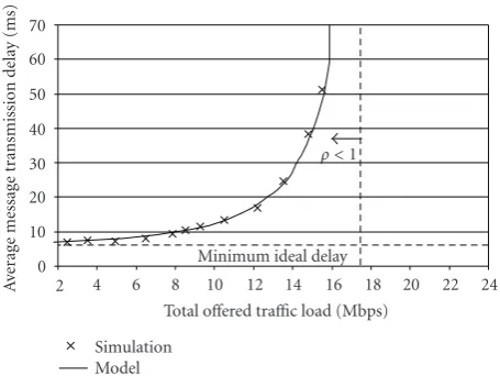
Figure 11: Average Message Transmission Delay (Model versus Simulation).

delay is close to the theoretical minimum, that is, the time required to transmit a data message almost without extra delay added by the MAC layer. The only delay cost is due to the control overhead associated to the MAC protocol, but almost without any contention as if a completely centralized network was present. Note that with the configuration of these simulations, the duration of a DQMAN frame is approximately equal to 800μs and thus the minimum time required for transmitting a message of 10 packets or fragments is 8 ms.

6. Comparison with the IEEE 802.11

MAC Protocol

The performance of DQMAN under non-saturation condi-tions is compared in this section to that of the DCF of the IEEE 802.11 Standard. In the light of a fair comparison, the 802.11 DCF has been also implemented in the same C++ simulator.

6.1. Scenario. We consider the same scenario as the one used for the model validation presented in the previous section. Three diﬀerent networks have been evaluated in this case:

(15)

(2) a network where the stations execute thebasic access modeof the IEEE 802.11,

(3) a network where the stations execute the collision avoidance mode of the IEEE 802.11 with RTS/CTS handshake between source and destination.

For the network running the IEEE 802.11 MAC protocol, the minimum backoﬀ window has been set to 64 and 3 backoﬀ stages have been considered. Accordingly, and in order to obtain a fair comparison between both protocols, the parameters of the MSP of DQMAN have been set toα=

64 andβ=0. The lengths of the RTS and CTS packets have been set to 20 and 14 bytes, respectively, and the duration of the DIFS and SIFS to 50μs and 10μs, respectively. In this case, a constant message length of 1500 bytes has been considered, which means that just one packet is transmitted once the channel is successfully seized.

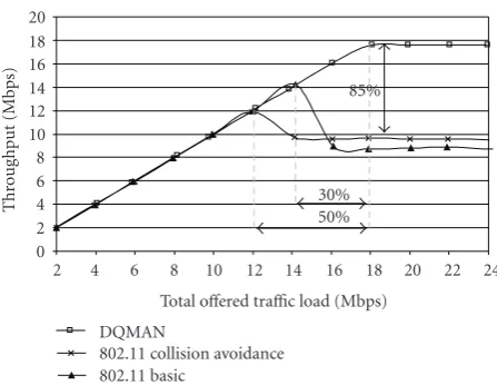
6.2. Results. The throughput of the network as a function of the total oﬀered traﬃc load to the network is depicted

in Figure 12. It is shown that DQMAN outperforms IEEE

802.11 in all cases. For low oﬀered loads, DQMAN and the IEEE 802.11 MAC protocol show similar throughput values, with a linear growth of the throughput of the network as the oﬀered load grows. In our layout, the network with the collision avoidance mechanism of the 802.11 Standard saturates approximately at 12 Mbps. Over that threshold, the performance drops to a stable value around 9.5 Mbps.

The basic access method shows a maximum throughput operational point close to the 14 Mbps. These values repre-sent an improved saturation throughput of 2 Mbps (17%) with respect to the collision avoidance mode. However, for higher offered loads, the throughput of the basic access model decreases asymptotically to a stable value of approx-imately 8.5 Mbps, which is below the saturation throughput of the collision avoidance access mode. The main reason for this performance is that the probability of collision increases with the offered traffic load. Therefore, the longer duration of collisions in the basic access mode yields lower throughput when compared to the collision avoidance mode where collisions are confined to control packets (RTS packets). On the other hand, DQMAN reaches the saturation conditions at an approximate traffic load of 17.8 Mbps and it remains stable at this value for higher traffic loads. This represents an improvement of 30% and 50% with respect to the peak of throughput attained by the collision avoidance and basic access modes of the standard, respectively. However, under heavy traffic conditions, DQMAN outperforms any of the two access modes of the standard in at least 85%. The reason for this improved performance of DQMAN resides in the fact that it eliminates backoffperiods devoted to the transmission of data and collision of data packets are completely avoided. Note that in DQMAN contention-based access is confined to the clustering phases.

The average message transmission delay is illustrated in

Figure 13and reinforces the previous discussion. The average

delay for the network executing the collision avoidance access mechanism gets unbounded for oﬀered traﬃc loads above 12 Mbps. The same happens with the basic access mode

0 2 4 6

Thr

o

ug

hpu

t

(Mbps)

8 10 12 14 16 18 20

2

802.11 collision avoidance DQMAN

802.11 basic

4 6 8 10

Total oﬀered traﬃc load (Mbps) 12 14

50% 30%

85%

16 18 20 22 24

Figure12: Throughput Comparison DQMAN versus 802.11.

0 5 10

A

ver

age

m

essage

tr

ansmission

dela

y

(ms)

15 20 25 30

2

802.11 collision avoidance DQMAN

802.11 basic

4 6 8 10

Total oﬀered traﬃc load (Mbps)

12 14 16 18 20 22 24

Figure13: Average Message Transmission Delay DQMAN versus 802.11.

over 14 Mbps, while DQMAN performs well in terms of delay up to 16 Mbps. It is worth mentioning that the three protocols provide a similar performance in terms of average transmission delay when the offered load is low. Indeed, this is an expected result. DQMAN switches smoothly from a random-based access to a reservation method as the traffic load grows. Therefore, when the traffic is low, both the standard and DQMAN operate similarly.

7. Conclusions

(16)

algorithm of a DQMAN station. Then, the average time spent at each state has been calculated by integrating classical queuing theory into the model. Combining the two analyses, the performance of the network has been evaluated in terms of throughput, average time spent in each mode of operation (idle, master, or slave), and average message transmission delay. In addition, computer link-level simulations have been used to validate the accuracy of the model and to show that DQMAN outperforms the IEEE 802.11 Standard in terms of throughput and average message transmission delay.

Our ongoing and future work is aimed at implementing the protocol in a testbed to evaluate the performance of DQMAN in a real network in the light of its commercial application.

Acknowledgments

This work was partially funded by the Research Projects NEWCOM++ (ICT-216715), R2D2 (CP6-013), CENTENO (TEC2008-06817-C02-02), and COOLNESS (218163-FP7-PEOPLE-2007-3-1-IAPP) and by Generalitat de Catalunya (2009-SGR-940).

References

[1] IEEE, Part 11: Wireless LAN Medium Access Control (MAC) and Physical Layer (PHY) Specifications, IEEE Std. 802.-11-99, August, 1999.

[2] Y. Xiao and J. Rosdahl, “Throughput and delay limits of IEEE 802.11,”IEEE Communications Letters, vol. 6, no. 8, pp. 355– 357, 2002.

[3] J. Alonso-Z´arate, E. Kartsakli, C. Skianis, C. Verikoukis, and L. Alonso, “Saturation throughput analysis of a cluster-based medium access control protocol for single-hop ad hoc wireless networks,”Simulation: Transactions of the Society for Modeling and Simulation International, vol. 84, no. 12, pp. 619–633, 2008.

[4] J. Alonso-Z´arate, E. Kartsakli, C. Verikoukis, A. Cateura, and L. Alonso, “A near-optimum cross-layered distributed queuing protocol for wireless LAN,” IEEE Wireless Communications, vol. 15, no. 1, Article ID 4454704, pp. 48–55, 2008.

[5] W. Xu and G. Campbell, “A near perfect stable random access protocol for a broadcast channel,” inProceedings of the IEEE International Conference on Communications (ICC ’92), vol. 1, pp. 370–374, 1992.

[6] J. Alonso-Z´arate, C. Verikoukis, E. Kartsakli, and L. Alonso, “Performance enhancement of DQMAN-based wireless ad hoc networks in multi-hop scenarios,” inProceedings of the 3rd International Symposium on Wireless Pervasive Computing (ISWPC ’08), pp. 425–429, Santorini, Greece, May 2008. [7] C. Prehofer and C. Bettstetter, “Self-organization in

commu-nication networks: principles and design paradigms,” IEEE Communications Magazine, vol. 43, no. 7, pp. 78–85, 2005. [8] J. Y. Yu and P. H. J. Chong, “A survey of clustering schemes for

mobile ad hoc networks,”IEEE Communications Surveys and Tutorials, vol. 7, no. 1, pp. 32–48, 2005.

[9] D. Wei and H. A. Chan, “A survey on cluster schemes in ad hoc wireless networks,” inProceedings of the 2nd International Conference on Mobile Technology, Applications and Systems, p. 62, GuangZhou, China, January 2005.

[10] C. Li, “Clustering in packet radio networks,” in Proceedings of the IEEE International Conference on Communications (ICC ’85), pp. 283–287, 1985.

[11] D. Wei and H. A. Chan, “A survey on cluster schemes in Ad Hoc wireless networks,” inProceedings of the 2nd International Conference on Mobile Technology, Applications and Systems, pp. 1–8, November 2005.

[12] T. Kwon, M. Gerla, V. K. Varma, M. Barton, and T. R. Hsing, “Eﬃcient flooding with passive clustering—an overhead-free selective forward mechanism for ad hoc/sensor networks,”

Proceedings of the IEEE, vol. 91, no. 8, pp. 1210–1220, 2003. [13] J. Alonso, C. Verikoukis, and L. Alonso, “Fairness

enhance-ment in a self-configuring cluster-based wireless ad hoc network,” inProceedings of the 8th International Symposium on Wireless Personal Multimedia Communications (WPMC ’05), Aalborg, Denmark, September 2005.

[14] G. Campbell, et al., “Method and apparatus for detecting col-lisions and controlling access to a communications channel,” US patent no. US6408009 B1, June 2002.

[15] L. Kleinrock,Queuing Systems, John Wiley & Sons, New York, NY, USA, 1976.

[16] G. Bianchi, “Performance analysis of the IEEE 802.11 dis-tributed coordination function,” IEEE Journal on Selected Areas in Communications, vol. 18, no. 3, pp. 535–547, 2000. [17] H. Wu, Y. Peng, K. Long, S. Cheng, and J. Ma, “Performance

of reliable transport protocol over IEEE 802.11 wireless LAN: analysis and enhancement,” in Proceedings of the Annual Joint Conference on the IEEE Computer and Communications Societies (INFOCOM ’02), pp. 599–607, June 2002.

[18] F. Alizadeh-Shabdiz and S. Subramaniam, “Analytical models for single-hop and multi-hop ad hoc networks,” Mobile Networks and Applications, vol. 11, no. 1, pp. 75–90, 2006. [19] J. Alonso-Z´arate, D. Gregoratti, P. Giotis, Ch. Verikoukis, and

L. Alonso, “Medium access control priority mechanism for a DQMAN-based wireless network,”IEEE Communications Letters, vol. 13, no. 7, pp. 495–497, 2009.

[20] L. Alonso, R. Agust´ı, and O. Sallent, “Near-optimum MAC protocol based on the distributed queueing random access protocol (DQRAP) for a CDMA mobile communication system,”IEEE Journal on Selected Areas in Communications, vol. 18, no. 9, pp. 1701–1718, 2000.

[21] J. Yeo, M. Youssef, and A. Agrawala, “Characterizing the IEEE 802.11 traﬃc: the wireless side,” Tech. Rep. CS-TR-4570, University of Maryland, College Park, 2004, http:// www.cs.umd.edu/Library/TRs/CS-TR-4570/CS-TR-4570.pdf. [22] IEEE Std. 802.11g, Supplement to Part 11: Wireless LAN