R E S E A R C H
Open Access
A class of quasi-variable mesh methods
based on off-step discretization for the
numerical solution of fourth-order
quasi-linear parabolic partial differential
equations
Ranjan Kumar Mohanty
1*and Deepti Kaur
2*Correspondence: [email protected] 1Department of Applied Mathematics, Faculty of Mathematics and Computer Science, South Asian University, Akbar Bhawan, Chanakyapuri, New Delhi 110021, India
Full list of author information is available at the end of the article
Abstract
Numerical schemes based on off-step discretization are developed to solve two classes of fourth-order time-dependent partial differential equations subjected to appropriate initial and boundary conditions. The difference methods reported here are second-order accurate in time and second-order accurate in space and, for a nonuniform grid, second-order accurate in time and third-order accurate in space. In case of a uniform grid, the second scheme is of order two in time and four in space. The presented methods split the original problem to a coupled system of two second-order equations and involve only three spatial grid points of a compact stencil without discretizing the boundary conditions. The linear stability of the presented methods has been examined, and it is shown that the proposed two-level finite difference method is unconditionally stable for a linear model problem. The new developed methods are directly applicable to fourth-order parabolic partial differential equations with singular coefficients, which is the main highlight of our work. The methods are successfully tested on singular problems. The proposed method is applied to find numerical solutions of the Euler-Bernoulli beam equation and complex fourth-order nonlinear equations like the good Boussinesq equation. Comparison of the obtained results with those for some earlier known methods show the superiority of the present approach.
Keywords: Euler-Bernoulli beam equation; off-step nodal points; quasi-variable mesh; finite difference method; successive tangential partial derivatives; good Boussinesq equation
1 Introduction
Consider the fourth-order quasi-linear parabolic partial differential equation (PDE)
A(x,t,u,uxx)
∂u
∂x +
∂u
∂t =f(x,t,u,ut,ux,uxx,uxxx), (x,t)∈, ()
where ={(x,t)|–∞<a<x<b<∞,t> }, equipped with the following initial and boundary conditions:
u(x, ) =u(x), ut(x, ) =u(x), a≤x≤b, (a)
and
u(a,t) =g(t), u(b,t) =g(t), t> , (b)
uxx(a,t) =h(t), uxx(b,t) =h(t), t> , (c)
where f,u,u,g,g,h, andh are functions of sufficient smoothness with required high-order derivatives.
Fourth-order PDEs arise in various mathematical models of physical problems in science and engineering such as vibrations of a homogenous beam, propagation of shallow water waves, fluid dynamics, surface diffusion of thin solid films, and deformation of beams [– ]. Jacob Bernoulli formulated the first consistent elasticity theory of thin beams, in which the curvature of an elastic beam at any point is proportional to the bending moment at that point. Based on his uncle’s elasticity theory, Daniel Bernoulli derived a PDE repre-senting the motion of a thin vibrating beam [, ]. Then, Leonard Euler extended and ap-plied Bernoulli’s theory to the loaded beams []. The Euler-Bernoulli beam equation is a fourth-order PDE governing the undamped transverse vibrations of a homogenous beam, in which the support does not contribute to the strain energy of the system and is set up as follows []:
∂
∂x
σ(x)∂
u
∂x
+μ(x)∂
u
∂t =p(x,t), (x,t)∈, ()
whereu(x,t) is the transverse displacement of each position of the beam,σ(x) > is the flexural rigidity,μ(x) > is the linear mass density,p(x,t) is the load per unit length, and
b–ais the length of the beam. The quantity uxx is the value of the bending moment of the beam. Equation () must be solved subject to the initial conditions (a) and simply supported boundary conditions (b)-(c). The solution of the Euler-Bernoulli beam equa-tion () is significant in various branches of engineering such as the construcequa-tion of flexible structures, the layout of robotic designs, and so on (see [, ]). The other time-dependent fourth-order PDE studied in the paper is the second-order Benjamin-Ono equation [, ] of the form
q∂
u
∂x +r
∂(u) ∂x +
∂u
∂t = , (x,t)∈, ()
leading to the existence of soliton solutions []. The general form of the good Boussinesq equation can be written as
∂u
∂t =
∂u
∂x +
∂u
∂x –
∂u
∂x, (x,t)∈. ()
It is one of the important models having numerous applications in several fields, for in-stance, ion-acoustic waves in plasma, magnetohydrodynamics waves in plasma, longitu-dinal dispersive waves in elastic rods, pressure waves in liquid-gas bubble mixtures, and so on (see [, ]). It describes shallow water waves propagating in both directions and possesses a highly complicated mechanism of solitary wave interaction [].
Another particular class of fourth-order nonlinear parabolic PDEs considered in this study is of the form
∂u
∂x–
∂u
∂x∂t+
∂u
∂t =g(x,t,u,ux,uxx–ut,uxxx–uxt), (x,t)∈, () subject to the initial and boundary conditions (a)-(c) (see []).
Owing to their great importance and wide range of applications, the attention of many physicists and mathematicians has been attracted to the studies of such problems. The closed-form solutions to fourth-order PDEs are necessary to know the qualitative behav-ior of natural processes and physical phenomena. But most fourth-order time-dependent PDEs have no closed-form solutions except for certain particular types of linear or quasi-linear equations. Therefore, construction of accurate numerical methods for finding ap-proximate solutions to these equations are of great significance. Among the entire arse-nal of numerical methods available to approximate a fourth-order PDE, such as the finite element method, spline collocation method, the finite difference method, is attractive be-cause of its relative ease of implementation, flexibility, and accuracy in the solution values. Higher-order methods yield not only comparable accuracy but also require much coarser discretization with greater computational efficiency. Apart from this, the advantage of de-veloping a compact scheme restricted to the patch of cells immediately surrounding any given grid point is its suitability to be used directly adjacent to the boundary without in-troducing any extra nodes outside the boundary of the domain. Higher-order difference approximations for one-space-dimensional nonlinear parabolic and hyperbolic differen-tial equations were discussed in [–]. A meshless numerical solution of hyperbolic PDEs using an improved localized radial basis functions collocation method was proposed in []. Recently, a new high-order compact implicit variable mesh discretization for one-space-dimensional unsteady quasi-linear biharmonic problem was developed in [].
alternating group explicit method achieving a better accuracy level. Later, Khanet al.[] reported a three-level difference method of accuracyO(k+h) for numerical solution of the Euler-Bernoulli equation by using a sextic spline in space and finite difference dis-cretization in time. Further, Caglar and Caglar [] considered a family of B-spline meth-ods to produce accurate numerical solution of the Euler-Bernoulli equation. Rashidinia and Mohammadi [] developed an approximation for finding the numerical solution of differential equation () by replacing the time derivative by a finite difference approxi-mation and the space derivative by sextic spline functions using off-step points to obtain three-level implicit methods of accuraciesO(k+h) andO(k+h). Mittal and Jain [] discussed two new methods for solving the Euler-Bernoulli equation using B-splines with redefined basis functions. Most recently, Mohammadi [] proposed a sextic B-spline col-location scheme for numerical solution of fourth-order time-dependent PDEs subjected to fixed and cantilever boundary conditions. Lai and Ma [] proposed a lattice Boltzmann model for the second-order Benjamin-Ono equation (). Numerous numerical methods have been proposed for solving the good Boussinesq equation () (see [–]). Recently, Siddiqi and Arshed [] developed a quintic B-spline collocation method for finding an approximate solution of the good Boussinesq equation.
The consideration of using off-step nodal points for discretization is motivated by the polar form of one space Laplacian operator∇≡∂/∂r+ (α/r)(∂/∂r), which has a singular coefficient associated with the first-order derivative term. Using only three grid points at each time level, three-level compact difference methods of order two in time and four in space for the solution of differential equation () for uniform mesh were reported by Mohanty and Evans [], but these methods fail at singular points, and a special technique was needed to solve singular problems. To this concern, in the present article, using the same number of grid points ( + + ) of a single compact cell, we have proposed two new off-step discretizations for the solution of the fourth-order quasi-linear PDE () having the foremost advantage that these are directly applicable to the singular problems without requiring any fictitious points. Recently, Mohanty and Kaur [] proposed an implicit high-order two-level finite difference scheme for the solution of particular type of fourth-high-order equation (). However, that scheme featured a major shortcoming that it is not directly applicable to the singular problems and requires a special treatment to handle singular points. In this paper, we have developed two new two-level unconditionally stable implicit methods using off-step nodal points for the solution of the differential equation (). The proposed new methods are convenient to implement at singular points without requiring any modification, and we do not need to discretize the boundary conditions, which is a main attraction.
2 Three-level quasi-variable mesh off-step discretization and derivation
For simplicity, we first consider the fourth-order nonlinear parabolic PDE of the form
A(x,t)∂
u
∂x+
∂u
∂t =f(x,t,u,ut,ux,uxx,uxxx), (x,t)∈. () We introduce the new variablevdefined as
v=∂
u
∂x.
Then equation () is reduced into an equivalent form of two second-order differential equations:
∂u
∂x =v, (x,t)∈, (a)
A(x,t)∂
v
∂x +
∂u
∂t =f(x,t,u,v,ut,ux,vx), (x,t)∈. (b) Since the value ofuandutis prescribed att= , this implies that the values of all succes-sive tangential partial derivativesux,uxx, . . . ofuare known att= . Sincev(x, ) =uxx(x, ), the value ofvis also known att= . Also, note that the values ofuandvare given atx=a
andx=b.
The associated initial and boundary conditions with (a)-(b) are
u(x, ) =u(x), v(x, ) =u(x),
ut(x, ) =u(x), a≤x≤b, (a)
u(a,t) =g(t), v(a,t) =h(t), t> , (b)
u(b,t) =g(t), v(b,t) =h(t), t> . (c)
In order to obtain a numerical solution of above initial boundary value problem, we superimpose on the solution domaina rectangular grid with spacinghl=xl–xl–,l= ()N+ , in thex-direction such thata=x<x<· · ·<xN <xN+=b,Nbeing a positive integer, andk=tj+–tj> in time direction. Spatial grid points are defined byxl=x+
l
i=hi,l= ()N+ , and time steps are given bytj=jk,j= , , , . . . ,J, whereJis a positive integer. The mesh ratio is denoted byηl= (hl+/hl) > ,l= ()N. The neighboring off-step points are defined asxl+/=xl+ηlhl andxl–/=xl–hl,l= ()N. Forηl= , it reduces to the uniform mesh case. Letujl,vjldenote approximate solution values ofu(x,t),v(x,t) at the grid point (xl,tj), andUlj,V
j
l be their exact solution values at the the grid point (xl,tj), respectively. ForE=A,Ax, andAxx, let the valuesE(xl,tj) be denoted by Ejl. For simplicity, we considerηl=η(a constant= ),l= ()N. Such a mesh is called a quasi-variable mesh.
At the grid point (xl,tj), forS=A,U, andV, we denote
Sab=
∂a+bS
Let
Similarly, approximations are defined for the solution variablev(x,t) at the grid point (xl,tj) by replacingUwithVin these expressions. Next, we define
respectively, whereTjl()=O(kh
The derivation of the numerical methods (a)-(b) is straightforward. So, we discuss in detail the derivation of the novel off-step discretization technique given by (a)-(b).
At the grid point (xl,tj), we let
Vjl=Vlj+θkV+
Finally, invoking the Taylor expansion and using (a)-(e) in (), we obtain
Fjl=Flj+k Further, by Taylor’s series expansion we may write
Ujl+– ( +η)Ujl+ηUjl–=Ul+j – ( +η)Ulj+ηUl–j +θη( +η)
l associated with (a) may be obtained asT j()
l =O(khl+hl) for arbitraryθ. In a similar manner, by the help of approximations (a)-(d), (a)-(b), (), and (b),
from (b) we obtain the local truncation errorTj
()
l associated with (b) as
We observe from () that for the proposed method (b) to be of accuracyO(k+kh we obtain the values of the parameters
a=b= – we need to modify our proposed difference methods (a)-(b) and (a)-(b). In this case, we make use of the following approximations in (a)-(b) and (a)-(b):
A=
Using approximations (a)-(d), the difference methods (a)-(b) and (a)-(b) retain their orders, and hence we obtain difference methods of orders O(k+hl) and
O(k+kh
A+
respectively, for arbitraryθ.
Note that for the constant mesh case, the difference method (a)-(b) is fourth-order accurate in space for a fixed value of the mesh ratio parameterλ=k/h.
3 Two-level off-step discretization strategy and truncation error analysis
In this section, we develop new quasi-variable mesh off-step finite difference methods for the differential equation () with initial and boundary conditions given by (a)-(c).
Let us introduce the new variablev(x,t) =uxx(x,t) –ut(x,t). Then we may rewrite the given PDE () in a coupled manner as
∂u implies that the values of their successive tangential derivatives are known on the bound-ary, that is, the values ofuxx(x, ) =u(x),ut(a,t) =g(t), andut(b,t) =g(t) are known exactly on the boundary.
The initial and boundary conditions associated with (a)-(b) can be written as
u(x, ) =u(x), v(x, ) =u(x) –u(x), a≤x≤b (a)
u(a,t) =g(t), v(a,t) =h(t) –g(t), u(b,t) =g(t),
v(b,t) =h(t) –g(t), t> . (b)
Let
tj=tj+τk, ()
where <τ < is a parameter to be suitably determined.
We discuss in detail the derivation of quasi-variable mesh finite difference method (a)-(b). In this section, at the grid point (xl,tj), we denote
The proposed differential equations (a)-(b) at the grid point (xl,tj) can be written as
U=U+V, (a)
In a similar manner,
Gjl±/=gxl,tj,Ulj±/,V
The following relations are obtained upon differentiating system (a)-(b) with respect totat the grid point (xl,tj):
U=U+V, (a)
V=V+E+HU+IV+JU+K V. (b)
By the help of approximations (a)-(f), from (b) we get
Using approximations (a)-(f) and (a)-(b), we obtain
Using relation (a) and Taylor series, the local truncation errorTlj() associated with (a) is obtained as
Thus, for the proposed difference method (b) to be of orderO(k+kh
l+hl), we must have
–η+ηS+ S= . ()
Substituting the values of S andS into () and equating to zero the coefficients of
U,V,U,V, andV, we obtain the following values of the parameters: (a)-(b) and (a)-(b) for the solution of differential equations (a)-(b) reduce to the following implicit difference methods of ordersO(k+h) andO(k+h):
4 Stability analysis using characteristic equation
Let us consider the singularly perturbed model equation
∂
u
∂x+
∂u
∂t =f(x,t), (x,t)∈, ()
where < is a small parameter. The proposed difference method (a)-(b) of or-derO(k+h) for the uniform mesh when applied to this equation results in the following scheme written in the matrix form:
The matricesS andT are N×N block tridiagonal,yis the N-component solution
vector, andwdenotes the Ncomponent column vector of known boundary values and
right-hand side function values of the block system (). The submatrices forSandTare given by
S= θ[, –, ], S= –hθ[, , ],
S= [, , ], S= λhθ[, –, ],
T= –[, –, ], T=h[, , ],
T= [, , ], T= –λh[, –, ],
where [a,b,c] is theN×Ntridiagonal matrix having eigenvaluesb+ √accos(φ),φ= (sπ)/((N+ )),s= ()N, andλ=k/his the mesh ratio parameter for the uniform mesh (forη= , that is, forhl+=hl=h). Here,u= (u,u, . . . ,uN)T andv= (v,v, . . . ,vN)Tare solution vectors.
The eigenvalues ofS,S,S, andSare given by –θsinφ, –hθ( – sinφ), – sinφ, and –λhθsinφ, respectively. Further, the eigenvalues ofT
,T,T, and
Tare given by sinφ,h( – sinφ), , and λhsinφ, respectively.
For discussing the stability of the differential equation (), we consider the homogenous part of the difference scheme (), which may be written as
yj+=I+S–Tyj–Izj, (a)
zj+=Iyj+ zj. (b)
We denote byεj=yj–Yjandεj=zj–Zjthe error vectors at thejth iterate (in the absence of round-off errors), where
Yj+=
U V
j+
, Zj+=Yj=
U V
j ,
UandV being exact solution vectors. We may write the error equation as
Ej+=
ε
ε
j+ =HEj,
where the amplification matrixHis given by
H=
I+S–T –I
I
.
The characteristic rootξof the matrixSsatisfies the following characteristic equation:
det
–θsinφ–ξ –hθ( – sinφ) – sinφ –λhθsinφ–ξ
which on simplification gives
ξ,= –
+λhθsinφ
±θ –λhsinφ– hθsinφ– –sinφ. ()
The characteristic rootρof the matrixTsatisfies the following characteristic equation:
det
–sinφ–ρ h( – sinφ)
λhsinφ–ρ
= ,
which gives
ρ= sinφ and ρ= λhsinφ. ()
Letνbe the eigenvalue ofS–T, whereξandρare eigenvalues ofSandTsatisfying () and (), respectively. Ifμdenotes the characteristic root of the amplification matrixH, then it satisfies the following characteristic equation:
det
+ν–μ –
–μ
= ,
which gives
μ– Wμ+ = , ()
whereW= +ν. Hence, we conclude that the difference method (a)-(b) is stable if
|W| ≤.
For stability of the particular fourth-order PDE, we consider the linear parabolic equa-tion of the form
∂u
∂x–
∂u
∂x∂t+
∂u
∂t =g(x,t), (x,t)∈. ()
Applying the method (a)-(b) of orderO(k+h) for the uniform mesh to the differ-ential equation (), we obtain the matrix equation
Qyj+=Ryj+l, ()
where
Q=
Q Q
Q
, R=
R R
R
, y=
u v
, l=
l
l
,
u,vare solution vectors, and the vectorsl,lconsist of homogenous functions, initial and boundary values of the block system (). The submatricesQ,Q,R, andRare given by
Q= [, , ] –
λ
[, –, ], Q=
k
R= [, , ] +
, respectively. Hence, the eigenvalues of the matricesQandRfor the difference method (a)-(b) are given by + λsinφand – λsinφ, respectively.
The amplification matrix of system () is given byQ–R. Since the matricesQ–andR commute each other, the eigenvaluesψ ofQ–Rare given by
ψ= – λsin
φ
+ λsinφ. ()
Since ≤sinφ≤, from () it is easy to verify that|ψ| ≤ for all variable anglesφand λ> . Hence the method (a)-(b) is unconditionally stable for the differential equa-tion ().
5 Application of the proposed difference methods to a linear singular equation
Let us consider a class of linear singular equations of the form
∇u+∂u
equipped with the initial and boundary conditions of the form (a)-(c). Equivalently, equation () can be written in a coupled form as
∂u
denotes the Laplacian operator in cylindrical and spherical coordinates, respectively, in one space dimension.
Applying the difference method (a)-(b) to the singular equation (), we obtain the following difference scheme of accuracyO(k+h
+ ( +η) Similarly, applying the difference method (a)-(b) to the singular equation (), we obtain the following difference scheme of accuracyO(k+kh
l+hl):
Note that the quasi-variable mesh difference schemes (a)-(b) and (a)-(b) for the solution of singular equation () do not have the terms involving /(rl±), so the singu-larity atr= is avoided, and thus these schemes can be very easily solved in the region [ <r< ]×[t> ] without any modification. The difference scheme of accuracyO(k+h) developed by Mohanty and Evans [] using three spatial grid points for the uniform mesh featured a major drawback: it is not directly applicable to the singular equation () since it contains the termFl–, so a singularity arises atl= sincer= and requires a special treatment to deal with the singular points. However, this is not the case with our proposed schemes sinceFl–
appears instead ofFl–, which is the major advantage of using off-step discretization.
6 Computational results
solution of nonlinear equations (see [, ]), and in each case, the iterations are termi-nated once the absolute error tolerance –is reached.
Note that the proposed difference methods (a)-(b) and (a)-(b) are three-level in time. The values ofuandvare known from the initial conditions. To begin any compu-tation, it is necessary to know the values ofuandvof required accuracy at the first time level, that is, att=k. Using the known values ofuandut att= , we can determine all their successive tangential partial derivatives att= , that is, the values of
∂ru l
∂xr ,
∂r+u l
∂xr∂t,
∂rv l
∂xr ,
∂r+v l
∂xr∂t, r= , , . . . ,
are known att= .
We use the following approximations foruandvof accuracyO(k) att=k:
Ul=Ul+kUtl+k
U
ttl+O
k, ()
Vl=Vl+kVtl +k
V
ttl+O
k. ()
The considered fourth-order quasi-linear PDE () may be written as
∂u
∂t = –A(x,t,u,uxx)
∂u
∂x +f(x,t,u,ut,ux,uxx,uxxx), (x,t)∈. () Differentiating () twice successively with respect toxand using the relationv=uxx, we get
∂v
∂t =
∂
∂x –A(x,t,u,uxx)
∂u
∂x +f(x,t,u,v,ut,ux,vx)
, (x,t)∈. ()
Using the initial values and their successive tangential partial derivatives in () and (), we can determine the values ofUttlandVttl. Finally, substituting these values into () and (), respectively, we can compute the values ofuandvof required accuracy att=k.
Throughout our computation (wherever not specified), we have used the time stepk= ./(N+ )for finding the solution att= . Since
b–a=xN+–x= (xN+–xN) + (xN–xN–) +· · ·+ (x–x) =hN++hN+· · ·+h =h
+η+η+· · ·+ηN,
so the first mesh spacing in thex-direction is obtained as
h=
(b–a)( –η)
–ηN+ , η= . ()
Thus, we can calculatehusing () and mesh lengths of the remaining subintervals in the
x-direction are computed by using the relationhl+=ηhl,l= ()N.
Example We consider the Euler-Bernoulli beam equation () in the following form [– ]:
∂u
∂x+
∂u
∂t =
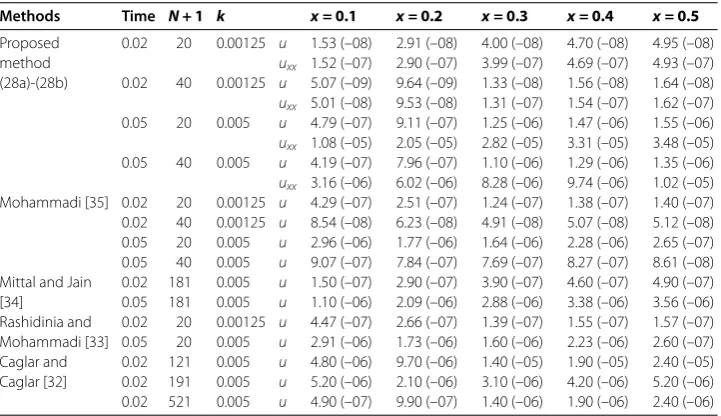
Table 1 The absolute errors in the displacementuand the bending momentuxxfor the
Euler-Bernoulli beam equation (68) for Example 1
Methods Time N + 1 k x = 0.1 x = 0.2 x = 0.3 x = 0.4 x = 0.5
Proposed method (28a)-(28b)
0.02 20 0.00125 u 1.53 (–08) 2.91 (–08) 4.00 (–08) 4.70 (–08) 4.95 (–08) uxx 1.52 (–07) 2.90 (–07) 3.99 (–07) 4.69 (–07) 4.93 (–07)
0.02 40 0.00125 u 5.07 (–09) 9.64 (–09) 1.33 (–08) 1.56 (–08) 1.64 (–08) uxx 5.01 (–08) 9.53 (–08) 1.31 (–07) 1.54 (–07) 1.62 (–07)
0.05 20 0.005 u 4.79 (–07) 9.11 (–07) 1.25 (–06) 1.47 (–06) 1.55 (–06) uxx 1.08 (–05) 2.05 (–05) 2.82 (–05) 3.31 (–05) 3.48 (–05)
0.05 40 0.005 u 4.19 (–07) 7.96 (–07) 1.10 (–06) 1.29 (–06) 1.35 (–06) uxx 3.16 (–06) 6.02 (–06) 8.28 (–06) 9.74 (–06) 1.02 (–05)
Mohammadi [35] 0.02 20 0.00125 u 4.29 (–07) 2.51 (–07) 1.24 (–07) 1.38 (–07) 1.40 (–07) 0.02 40 0.00125 u 8.54 (–08) 6.23 (–08) 4.91 (–08) 5.07 (–08) 5.12 (–08) 0.05 20 0.005 u 2.96 (–06) 1.77 (–06) 1.64 (–06) 2.28 (–06) 2.65 (–07) 0.05 40 0.005 u 9.07 (–07) 7.84 (–07) 7.69 (–07) 8.27 (–07) 8.61 (–08) Mittal and Jain
[34]
0.02 181 0.005 u 1.50 (–07) 2.90 (–07) 3.90 (–07) 4.60 (–07) 4.90 (–07) 0.05 181 0.005 u 1.10 (–06) 2.09 (–06) 2.88 (–06) 3.38 (–06) 3.56 (–06) Rashidinia and
Mohammadi [33]
0.02 20 0.00125 u 4.47 (–07) 2.66 (–07) 1.39 (–07) 1.55 (–07) 1.57 (–07) 0.05 20 0.005 u 2.91 (–06) 1.73 (–06) 1.60 (–06) 2.23 (–06) 2.60 (–07) Caglar and
Caglar [32]
0.02 121 0.005 u 4.80 (–06) 9.70 (–06) 1.40 (–05) 1.90 (–05) 2.40 (–05) 0.02 191 0.005 u 5.20 (–06) 2.10 (–06) 3.10 (–06) 4.20 (–06) 5.20 (–06) 0.02 521 0.005 u 4.90 (–07) 9.90 (–07) 1.40 (–06) 1.90 (–06) 2.40 (–06)
The exact solution of this problem is
u(x,t) =sinπxcost.
We have solved this problem by the proposed method (a)-(b) withh= ., . and
k= ., .. The absolute errors in the displacementuand the bending moment
uxxat particular pointsx= ., ., ., ., . are computed and reported in Table for different time levelst= . andt= . using and time steps, respectively. We have compared our results with the results in [–], and it is evident from Table that the proposed method (a)-(b) provides relatively more accurate solutions in comparison to the other existing methods. Figure (a) and (b) give a comparison of the plots of the exact and numerical solutions withh= . andk= . fort= to ..
Example We consider the following nonhomogenous fourth-order parabolic equa-tion []:
∂u
∂t + ( +x)
∂u
∂x =
x+x– !x
cost, <x< ,t> . ()
The exact solution is
u(x,t) = !x
cost.
Figure 1 Example 1: The graph of numerical and exact solutions forh= 0.025 andk= 0.005.
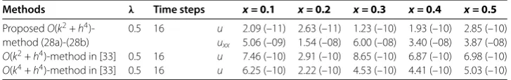
Table 2 The absolute errors for the nonhomogenous fourth-order parabolic equation (69), Example 2
Methods λ Time steps x = 0.1 x = 0.2 x = 0.3 x = 0.4 x = 0.5
ProposedO(k2+h4
)-method (28a)-(28b)
0.5 16 u 2.09 (–11) 2.63 (–11) 1.23 (–10) 1.93 (–10) 2.85 (–10) uxx 5.06 (–09) 1.54 (–08) 6.00 (–08) 3.40 (–08) 3.87 (–08)
O(k2+h4)-method in [33] 0.5 16 u 7.46 (–10) 2.91 (–10) 8.65 (–10) 6.87 (–10) 6.98 (–10)
O(k4+h4)-method in [33] 0.5 16 u 6.25 (–10) 2.22 (–10) 4.53 (–10) 4.41 (–10) 5.03 (–10)
Example We seek the numerical solution of the following homogenous variable coeffi-cient problem [, , ]:
x+ x
∂u
∂x+
∂u
∂t = ,
<x< ,t> . ()
The exact solution is
u(x,t) =
+ x
sint.
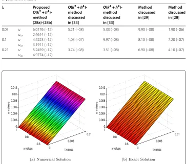
In order to compare the results obtained using our proposed methods with those of the existing methods [, , ], we have solved this problem using method (a)-(b) with
h= . andk= ., ., . using , , and time steps, respec-tively. The maximum absolute relative errors defined as
maxU j l–u
j l
Ulj
, l= ()N,
Table 3 The Maximum absolute relative errors for Example 3 att= 0.01 for various values of
λ(uniform mesh)
λ Proposed
O(k2+ h4)
-method (28a)-(28b)
O(k2+ h4)
-method discussed in [33]
O(k4+ h4)
-method discussed in [33]
Method discussed in [29]
Method discussed in [28]
0.05 u 6.0176 (–12) 5.21 (–08) 5.33 (–08) 9.90 (–08) 1.90 (–06)
uxx 2.4614 (–12)
0.1 u 4.4223 (–12) 1.03 (–07) 9.97 (–08) 8.10 (–08) 7.20 (–07)
uxx 3.1911 (–12)
0.25 u 5.2459 (–12) 3.74 (–08) 3.51 (–08) 6.90 (–08) 4.10 (–07)
uxx 4.9774 (–12)
Figure 2 Example 3: The graph of numerical and exact solutions forλ= 0.1,h= 0.05, andk= 0.00025 fort= 0 to 0.01.
Example We consider the singularly perturbed problem of the form
∂
u
∂x+
∂u
∂t =f(x,t), <, <x< ,t> . ()
The exact solution is
u(x,t) =e–πtsinπx.
The maximum absolute errors (MAEs) using methods (a)-(b) and (a)-(b) are tabulated in Table att= for various values of.
Table 4 The MAEs for Example 4 att= 1.0 for a fixedλ= (k/h2) = 1.6 (uniform mesh)
h O(k2+ h4)-method (28a)-(28b) O(k2+ h2)-method (27a)-(27b)
= 0.1 = 0.01 = 0.001 = 0.1 = 0.01 = 0.001
1/8 u 3.0988 (–04) 2.9825 (–05) 3.5010 (–06) 3.2430 (–02) 1.0781 (–02) 1.1932 (–03) uxx 2.4409 (–03) 3.8680 (–04) 4.4212 (–05) 3.9514 (–01) 1.1690 (–01) 1.2865 (–02)
1/16 u 1.9387 (–05) 1.8905 (–06) 2.2211 (–07) 8.0703 (–03) 2.7648 (–03) 3.0660 (–04) uxx 1.5294 (–04) 2.4412 (–05) 2.7933 (–06) 9.9261 (–02) 3.0176 (–02) 3.3273 (–03)
1/32 u 1.2121 (–06) 1.1856 (–07) 1.3934 (–08) 2.0148 (–03) 6.9554 (–04) 7.7174 (–05) uxx 9.5655 (–06) 1.5293 (–06) 1.7506 (–07) 2.4840 (–02) 7.6039 (–03) 8.3890 (–04)
Table 5 The MAEs for Example 5 att= 1.0,η= 0.94 (quasi-variable mesh)
N + 1 O(k2+ k2h
l+ h3l)-method (16a)-(16b) O(k2+ h2l)-method (15a)-(15b)
α= 1 α= 2 α= 1 α= 2
8 u 1.8743 (–04) 5.4079 (–04) 3.6061 (–03) 8.7376 (–03)
urr 1.4353 (–03) 8.2498 (–03) 8.6067 (–02) 7.9741 (–02)
16 u 1.7017 (–05) 4.5019 (–05) 6.8621 (–04) 1.6912 (–03)
urr 1.5498 (–04) 1.3071 (–03) 2.6282 (–02) 4.7895 (–02)
32 u 3.1833 (–06) 7.4946 (–06) 1.2889 (–04) 3.5410 (–04)
urr 5.1980 (–05) 4.3430 (–04) 1.1033 (–02) 3.0090 (–02)
Figure 3 Example 5: The graph of numerical and exact solutions forα= 1,η= 0.94, andN+ 1 = 8 for
t= 0 to 1.0.
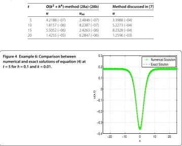
Example We consider the second-order Benjamin-Ono equation () withq= and
r= –. Fuet al.[] constructed the exact periodic solutions of equation () for the above parameters using the Jacobi elliptic function expansion method having the form
u(x,t) = r
– l+ ltanhl(x–rt).
Table 6 The MAEs for the second-order Benjamin-Ono equation (4) withq= 1,r= –1, Example 6 at various time levels forh= 0.1,k= 0.01
t O(k2+ h4)-method (28a)-(28b) Method discussed in [7]
u uxx u
5 4.2188 (–07) 2.4846 (–07) 3.3988 (–04) 10 1.8157 (–06) 8.2387 (–07) 5.2273 (–04) 15 5.5052 (–06) 2.4263 (–06) 8.2328 (–04) 20 1.4255 (–05) 6.2847 (–06) 1.2596 (–03)
Figure 4 Example 6: Comparison between numerical and exact solutions of equation (4) at
t= 5 forh= 0.1 andk= 0.01.
Table 7 The MAEs for the good Boussinesq equation (5), Example 7 at various time levels for a uniform mesh withk= 0.05
t Parameters O(k2+ h4)-method
(28a)-(28b)
Collocation method discussed in [36]
u uxx u
0.5 h= 1/40 x0= 30 8.1007 (–07) 4.4585 (–06) 8.2943 (–07)
1.0 h= 1/60 x0= 40 7.6030 (–09) 3.1598 (–08) 7.3326 (–09)
1.5 h= 1/80 x0= 50 5.8974 (–11) 2.0970 (–09) 6.4525 (–11)
2.0 h= 1/100 x0= 60 2.9068 (–13) 3.2836 (–13) 5.2066 (–13)
Example We consider the good Boussinesq equation () on the domain –≤x≤ with the following exact solution []:
u(x,t) = –Asech A
(x–ct+x)
–
b+
.
This exact solution represents a solitary wave with amplitudeAlocated initially atx=x and moving to the right or left corresponding to the sign of the velocityc. If cis posi-tive (negaposi-tive), then the solitary wave moves to the right (left). For comparison with [], we first choose the parametersA,b, andcsimilar to [], that is,A= .,b= –, and
Table 8 The MAEs for Example 8 att= 1.0,η= 0.92 (quasi-variable mesh)
N + 1 O(k2+ k2h
l+ h3l)-method (16a)-(16b) O(k2+ h 2
l)-method (15a)-(15b)
α= 10 α= 20 α= 40 α= 10 α= 20 α= 40
8 u 3.3667 (–05) 7.7683 (–05) 1.7212 (–02) 2.6072 (–04) 3.0874 (–04) 2.6133 (–02) uxx 3.3298 (–04) 7.6915 (–04) 1.7290 (–01) 2.3571 (–04) 7.0446 (–04) 2.5645 (–01)
16 u 2.1139 (–06) 4.7259 (–06) 1.0805 (–03) 8.6976 (–05) 1.0909 (–04) 9.5763 (–03) uxx 2.1334 (–05) 4.7049 (–05) 1.0817 (–02) 1.2171 (–04) 3.4424 (–04) 9.4655 (–02)
32 u 1.3319 (–07) 2.7901 (–07) 7.8958 (–05) 4.1496 (–05) 5.1293 (–05) 3.9491 (–03) uxx 1.5345 (–06) 2.9686 (–06) 7.9178 (–04) 5.4398 (–05) 1.5469 (–04) 3.9160 (–02)
Figure 5 Example 8: The graph of numerical and exact solutions forα= 20,η= 0.92 andN+ 1 = 8 for
t= 0 to 1.0.
Example We compute the approximate solution of the following quasi-linear equation:
+u+uxx∂
u
∂x+
∂u
∂t =αu(ux–uxx) +f(x,t), <x< ,t> . ()
The exact solution is
u(x,t) =coshxsinht.
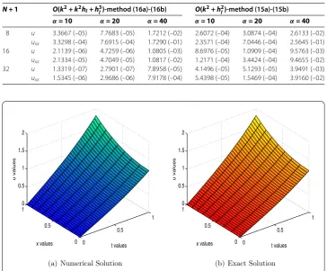
The MAEs are tabulated in Table att= forη= . and for various values ofα. The D graphs of numerical solution using method (a)-(b) vs exact solution are plotted in Figure (a) and (b), respectively, for <x< fromt= to .
Example We consider the following particular type of fourth-order nonlinear parabolic equations:
∂u
∂x–
∂u
∂x∂t+
∂u
∂t =αu(uxx–ut) +g(x,t), <x< ,t> . ()
The exact solution is
Table 9 The MAEs for Example 9 att= 4.0,η= 0.92 (quasi-variable mesh)
N + 1 O(k2+ kh
l+ h3l)-method (37a)-(37b) O(k2+ h 2
l)-method (36a)-(36b)
α= 1 α= 5 α= 10 α= 1 α= 5 α= 10
8 u 2.5627 (–05) 3.5373 (–05) 7.1052 (–05) 1.1611 (–04) 1.1059 (–04) 8.9291 (–05) uxx–ut 2.8854 (–05) 8.8904 (–05) 4.3557 (–04) 1.6636 (–05) 4.6297 (–05) 2.4532 (–04)
16 u 1.6009 (–06) 2.2252 (–06) 4.5252 (–06) 4.3184 (–05) 4.3903 (–05) 4.6318 (–05) uxx–ut 1.8900 (–06) 5.7189 (–06) 2.8222 (–05) 2.0745 (–06) 8.1349 (–06) 3.5144 (–05)
32 u 9.1931 (–08) 1.3617 (–07) 2.9842 (–07) 2.1699 (–05) 2.2259 (–05) 2.4254 (–05) uxx–ut 1.4804 (–07) 4.2072 (–07) 2.0094 (–06) 1.7714 (–06) 6.1484 (–06) 2.7953 (–05)
Table 10 The MAEs for Example 10 att= 1.0 for a fixedλ= (k/h2) = 1.6 (uniform mesh)
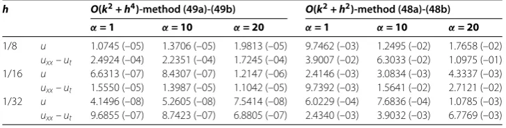
h O(k2+ h4)-method (49a)-(49b) O(k2+ h2)-method (48a)-(48b)
α= 1 α= 10 α= 20 α= 1 α= 10 α= 20
1/8 u 1.0745 (–05) 1.3706 (–05) 1.9813 (–05) 9.7462 (–03) 1.2495 (–02) 1.7658 (–02) uxx–ut 2.4924 (–04) 2.2351 (–04) 1.7245 (–04) 3.9007 (–02) 6.3033 (–02) 1.0975 (–01)
1/16 u 6.6313 (–07) 8.4307 (–07) 1.2147 (–06) 2.4146 (–03) 3.0834 (–03) 4.3337 (–03) uxx–ut 1.5550 (–05) 1.3987 (–05) 1.1042 (–05) 9.7392 (–03) 1.5641 (–02) 2.7121 (–02)
1/32 u 4.1496 (–08) 5.2605 (–08) 7.5414 (–08) 6.0229 (–04) 7.6836 (–04) 1.0785 (–03) uxx–ut 9.6855 (–07) 8.7423 (–07) 6.8805 (–07) 2.4340 (–03) 3.9032 (–03) 6.7769 (–03)
The MAEs using method (a)-(b) and (a)-(b) are reported in Table forη= . att= using the time stepk= ./(N+ )for various values ofα.
Example We consider the particular type of fourth-order singular equation of the form:
∂u
∂x–
∂u
∂x∂t+
∂u
∂t =
(uxx–ut)
x +
α
xu+g(x,t), <x< ,t> . ()
The exact solution is
u=e–tsinπx.
The MAEs using method (a)-(b) and (a)-(b) are reported in Table att= for various values ofα.
7 Conclusions
In this paper, we propose finite difference approximations for the fourth-order time-dependent parabolic PDEs () and (). The methods were tested on several examples taken from the literature to observe the accuracy and efficiency of the new methods. The results illustrate that the errors in the numerical solution obtained by the current approach are smaller than those obtained by earlier research studies. The main conclusions are:
second-order Benjamin-Ono equation and is in good agreement with [] for the nonlin-ear good Boussinesq equation.
(ii) Compact stencil: The finite difference methods discussed here are based only on three spatial grid points. In each time step, every iteration involves solving a tridiagonal system.
(iii)No Ghost points: The boundary conditions are incorporated in a natural way without the use of any extra nodes or special schemes adjacent to the boundary, thereby eliminating the usual complexity encountered with the difference methods.
(iv)Directly applicable to singular problems: The existing fourth-order implicit differ-ence method of [] for solving the fourth-order quasi-linear parabolic equation () is not directly applicable to problems in polar coordinates and requires a special technique to handle singular points because of the presence of the terms of the form /rl–, which give rise to singularity atl= asr= . In the present paper, by using off-step nodal points the singularity atr= is avoided, which enables a direct application of the proposed sta-ble methods for finding the numerical solution of fourth-order parabolic equations with singular coefficients.
(v)Unconditional stability of the two-level method: The two-level implicit methods for the particular type of the fourth-order parabolic PDE () are unconditionally stable. Thus, the time step can be considerably large, which is extremely useful when the problem is solved on a long time interval. In Example , the maximum absolute errors has been cal-culated at large time levelst= , , , , and in Example , the errors are computed at
t= . The accuracy of the schemes is not degraded at large time intervals.
Also, the numerical solution ofuxx, in case of solution of () and the one-dimensional time-dependent Laplacianuxx–ut and in case of solution of (), which are quite often of interest in various applied problems, are computed as a byproduct of the proposed methods. We are currently working on extension of these methods to solve D and D fourth-order nonlinear parabolic PDEs. Application of these new methods to some more physical problems in science and engineering will be the content of our further research.
Competing interests
The authors declare that they have no competing interest.
Authors’ contributions
RKM discussed the three-level quasi-variable mesh method and partly stability analysis. DK discussed the two-level implicit method, application to singular problems, and partly stability analysis. DK also carried out the computational work. All the authors read and approved the final manuscript.
Author details
1Department of Applied Mathematics, Faculty of Mathematics and Computer Science, South Asian University, Akbar Bhawan, Chanakyapuri, New Delhi 110021, India.2Department of Mathematics, Faculty of Mathematical Sciences, University of Delhi, Delhi, 110007, India.
Acknowledgements
The authors thank the reviewers for their valuable comments and suggestions, which substantially improved the standard of the paper.
Received: 14 September 2016 Accepted: 29 November 2016 References
1. Gorman, DJ: Free Vibrations Analysis of Beams and Shafts. Wiley, New York (1975) 2. Meirovitch, L: Principles and Techniques of Vibrations. Prentice Hall, New Jersey (1997)
3. Debnath, L: Nonlinear Partial Differential Equations for Scientists and Engineers. Birkhauser, Boston (1997) 4. Hereman, W, Banerjee, PP, Korpel, A, Assanto, G: Exact solitary wave solutions of non-linear evolution and wave
5. Xu, ZH, Xian, DQ, Chen, HL: New periodic solitary-wave solutions for the Benjamin-Ono equation. Appl. Math. Comput.215, 4439-4442 (2010)
6. Soh, CW: Euler-Bernoulli beams from a symmetry standpoint-characterization of equivalent equations. J. Math. Anal. Appl.345, 387-395 (2008)
7. Lai, H, Ma, C: The lattice Boltzmann model for the second-order Benjamin-Ono equations. J. Stat. Mech.,2010P04011 (2010)
8. Bratsos, AG: The solution of the Boussinesq equation using the method of lines. Comput. Methods Appl. Mech. Eng.
157, 33-44 (1998)
9. Ismail, MS, Bratsos, AG: A predictor-corrector scheme for the numerical solution of the Boussinesq equation. J. Appl. Math. Comput.13, 11-27 (2003)
10. Dehghan, M, Salehi, R: A meshless based numerical technique for traveling solitary wave solution of Boussinesq equation. Appl. Math. Model.36, 1939-1956 (2012)
11. Mohanty, RK, Kaur, D: High accuracy implicit variable mesh methods for numerical study of special types of fourth order non-linear parabolic equations. Appl. Math. Comput.273, 678-696 (2016)
12. Jain, MK, Jain, RK, Mohanty, RK: A fourth order difference method for the one-dimensional general quasilinear parabolic partial differential equation. Numer. Methods Partial Differ. Equ.6, 311-319 (1990)
13. Mohanty, RK, Jain, MK, Kumar, D: Single cell finite difference approximations ofO(kh2+h4) for∂u/∂xfor one space dimensional nonlinear parabolic equation. Numer. Methods Partial Differ. Equ.16, 408-415 (2000)
14. Mohanty, RK, Karaa, S, Arora, U: AnO(k2+kh2+h4) arithmetic average discretization for the solution of 1-D nonlinear parabolic equations. Numer. Methods Partial Differ. Equ.23, 640-651 (2007)
15. Mohanty, RK: An implicit high accuracy variable mesh scheme for 1-D non-linear singular parabolic partial differential equations. Appl. Math. Comput.186, 219-229 (2007)
16. Mohanty, RK, Kumar, R: A new fast algorithm based on half-step discretization for one space dimensional quasilinear hyperbolic equations. Appl. Math. Comput.244, 624-641 (2014)
17. Mohanty, RK, Gopal, V: High accuracy non-polynomial spline in compression method for one-space dimensional quasi-linear hyperbolic equations with significant first order space derivative term. Appl. Math. Comput.238, 250-265 (2014)
18. Mohanty, RK, Jha, N, Kumar, R: A new variable mesh method based on non-polynomial spline in compression approximations for 1D quasilinear hyperbolic equations. Adv. Differ. Equ.2015337 (2015)
19. Talwar, J, Mohanty, RK, Singh, S: A new spline in compression approximation for one space dimensional quasilinear parabolic equations on a variable mesh. Appl. Math. Comput.260, 82-96 (2015)
20. Talwar, J, Mohanty, RK, Singh, S: A new algorithm based on spline in tension approximation for 1D quasi-linear parabolic equations on a variable mesh. Int. J. Comput. Math.93, 1771-1786 (2016)
21. Siraj-ul-Islam, Vertnik, R, Šarlen, B: Local radial basis function collocation method along with explicit time stepping for hyperbolic partial differential equations. Appl. Numer. Math.67, 136-151 (2013)
22. Mohanty, RK, Kaur, D: Numerov type variable mesh approximations for 1D unsteady quasi-linear biharmonic problem: application to Kuramoto-Sivashinsky equation. Numer. Algorithms (2016). doi:10.1007/s11075-016-0154-3 23. Conte, SD: A stable implicit finite difference approximation to a fourth order parabolic equation. J. Assoc. Comput.
Mech.4, 18-23 (1957)
24. Crandall, SH: Optimum recurrence formulas for a fourth order parabolic partial differential equation. J. Assoc. Comput. Mach.4, 467-471 (1957)
25. Evans, DJ: A stable explicit method for the finite difference solution of a fourth order parabolic partial differential equation. Comput. J.8, 280-287 (1965)
26. Fairweather, G, Gourley, AR: Some stable difference approximations to a fourth order parabolic partial differential equation. Math. Comput.21, 1-11 (1967)
27. Collatz, L: Hermitian methods for initial value problems in partial differential equations. In: Miller, JJH (ed.) Topics in Numerical Analysis, pp. 41-61. Academic Press, New York (1973)
28. Andrade, C, McKee, S: High accuracy A.D.I methods for fourth-order parabolic equations with variable coefficients. J. Comput. Appl. Math.3, 11-14 (1977)
29. Twizell, EH, Khaliq, AQM: A difference scheme with high accuracy in time for fourth order parabolic equations. Comput. Methods Appl. Mech. Eng.41, 91-104 (1983)
30. Evans, DJ, Yousif, WS: A note on solving the fourth-order parabolic equation by the AGE method. Int. J. Comput. Math.40, 93-97 (1991)
31. Khan, A, Khan, I, Aziz, T: Sextic spline solution for solving a fourth-order parabolic partial differential equation. Int. J. Comput. Math.82, 871-879 (2005)
32. Caglar, H, Caglar, N: Fifth-degree B-spline solution for a fourth-order parabolic partial differential equations. Appl. Math. Comput.201, 597-603 (2008)
33. Rashidinia, J, Mohammadi, R: Sextic spline solution of variable coefficient fourth-order parabolic equations. Int. J. Comput. Math.87, 3443-3454 (2010)
34. Mittal, RC, Jain, RK: B-splines methods with redefined basis functions for solving fourth order parabolic partial differential equations. Appl. Math. Comput.217, 9741-9755 (2011)
35. Mohammadi, R: Sextic B-spline collocation method for solving Euler-Bernoulli beam models. Appl. Math. Comput.
241, 151-166 (2014)
36. Siddiqi, SS, Arshed, S: Quintic B-spline for the numerical solution of the good Boussinesq equation. J. Egypt. Math. Soc.22, 209-213 (2014)
37. Mohanty, RK, Evans, DJ: The numerical solution of fourth order mildly qausi-linear parabolic initial boundary value problem of second kind. Int. J. Comput. Math.80, 1147-1159 (2003)
38. Kelly, CT: Iterative Methods for Linear and Non-linear Equations. SIAM, Philadelphia (1995) 39. Varga, RS: Matrix Iterative Analysis. Springer, New York (2000)